Analysis and Forecasting of the Carbon Price in China’s Regional Carbon Markets Based on Fast Ensemble Empirical Mode Decomposition, Phase Space Reconstruction, and an Improved Extreme Learning Machine

Abstract

With the development of the carbon market in China, research on the carbon price has received more and more attention in related fields. However, due to its nonlinearity and instability, the carbon price is undoubtedly difficult to predict using a single model. This paper proposes a new hybrid model for carbon price forecasting that combines fast ensemble empirical mode decomposition, sample entropy, phase space reconstruction, a partial autocorrelation function, and an extreme learning machine that has been improved by particle swarm optimization. The original carbon price series is decomposed using the fast ensemble empirical mode decomposition and sample entropy methods, which eliminate noise interference. Then, the phase space reconstruction and partial autocorrelation function methods are combined to determine the input and output variables in the forecasting models. An extreme learning machine optimized by particle swarm optimization was employed to forecast carbon prices. An empirical study based on carbon prices in three typical regional carbon markets in China found that this new hybrid model performed better than other comparable models.

1. Introduction

Nowadays, climate change has seriously threatened sustainable human development. Especially, China, as the world’s biggest emitter of CO₂, is particularly concerned in this regard [1]. In order to actively implement the Paris Agreement and to contribute to the fight against climate change, China has committed to reducing its carbon intensity by 40–45% per unit of GDP whilst increasing the share of non-fossil energy consumption to 15% by the year of 2020. Since the introduction of the Emissions Trading System (ETS) by the European Union (E.U.) in 2005, carbon emissions trading has become an important market tool for responding to climate change as well as a long-term mechanism to address pollution problems. Advancing with the times, China has successfully established regional pilots for carbon emissions trading and has currently formed eight regional carbon markets, consisting of three provinces and five cities. Moreover, in the carbon trading market, an important corollary factor is carbon price prediction, which helps to reflect the carbon reduction performance and market value [2]. It is certain that an accurate and a rational prediction of carbon prices would allow us to understand the pattern of carbon price variations and avoid risks in investments [3]. Therefore, it is meaningful to be concerned with scientific methods for predicting carbon prices in China. In addition, carbon prices in China’s regional markets are time-series-connected with historical data, which also makes it possible to deliver an accurate prediction by using the model that is presented in this paper.

While early-stage research has been conducted on a qualitative analysis of China’s carbon market [4,5], more and more carbon price prediction methods have emerged in recent studies. They can be classified into two types that are focused on modeling and forecasting the carbon price volatility: mathematical statistical models and artificial neural networks. The conventional mathematical statistical models include difference-in-difference (DID), the vector auto-regression model (VAR), the autoregressive integrated moving average (ARIMA), and generalized autoregressive conditional heteroscedasticity (GARCH) models. Huang [6] proved that carbon emission trading has a significant and sustained promotion effect on carbon emission reductions by using the difference-in-difference method. Zeng et al. [7] employed a structural vector autoregressive (SVAR) model for exploring the dynamic relationships among the carbon emission allowance price, the regional economy, and energy prices in Beijing. Their empirical research results showed that, instead of the energy price, the historical carbon allowance price series was the major influencing factor on the carbon price. Zhu and Wei [8] examined the forecasting ability of three hybrid ARIMA models under the E.U. ETS. However, the ARIMA model requires a stable time series, which obviously renders it unsuitable for the direct prediction of a carbon price time series. Notably, the different GARCH-type models are popular in this field. Xia [9] studied the carbon price volatility of five pilot cities in China with the AR-GARCH (1,1) model. The results of experiments showed high consistency. Byun and Cho [10] compared three methods to predict the related volatility, and concluded that the GARCH-type models were the most suitable method. However, Zhang et al. [11] found that GARCH-type models are only satisfactory for in-sample forecasting and have limited significance for out-of-sample results. As described in the abovementioned studies, a single statistical model may not satisfy the condition of flexibility for an appropriate simulation due to the dynamic characteristics of carbon price volatility.

Today, with the growing data volume and algorithms’ ability to learn, machine learning algorithms are prevailing. The most essential feature of machine learning is to learn the data, which means to build a system to parse data so as to excavate the laws that hold between the data. The main advantage of a machine learning algorithm is that it can consider multiple attributes or features at one time and capture the hidden relationship between them that is difficult for a statistical model to reveal [12,13,14,15,16,17]. Compared with a traditional statistical model, machine learning algorithms have a stronger self-learning ability, a generalization ability, fast calculation speed, an associative memory ability that can fit a nonlinear relationship, and more flexible applicability to the amount of sample data. Based on these advantages, machine learning algorithms are applied in many fields [18,19,20,21,22,23,24]. For example, many algorithms have been developed to predict carbon prices, such as the back propagation neural network (BPNN), the support vector machine (SVM), and the radial basis function neural network (RBF). Liu and Sun [25] applied a BPNN to forecast the carbon price and the carbon trading volume in Shanghai. Zhang et al. [26] proposed a grey neural network improved by the ant colony algorithm (GNN-ACA) for carbon spot price forecasting. The results showed that the selected model performed significantly better than single ARIMA and least squares support vector machine (LSSVM) models by using data collected from the E.U. ETS. Tsai [27] proposed a carbon price forecasting system using the radial basis function neural network (RBF), which can supply precise and real-time predictions of carbon prices. Moreover, the SVM and LSSVM, individually or in combination with plenty of other algorithms, have been widely adopted to predict the carbon trading price. Gao and Li [28] compared some different prediction models in accordance with the daily EU emission allowance (EUA) futures prices from March 2008 to September 2013 (DEC12). The results indicated that the proposed EMD-PSO-SVM model performed better than other artificial neural networks (ANNs) in carbon price forecasting. Razak et al. [29] and Zhu et al. [30] used LSSVM as their main forecasting model. Their conclusions indicated that the LSSVM model seems to be a superior method for forecasting highly nonlinear and nonstationary carbon prices.

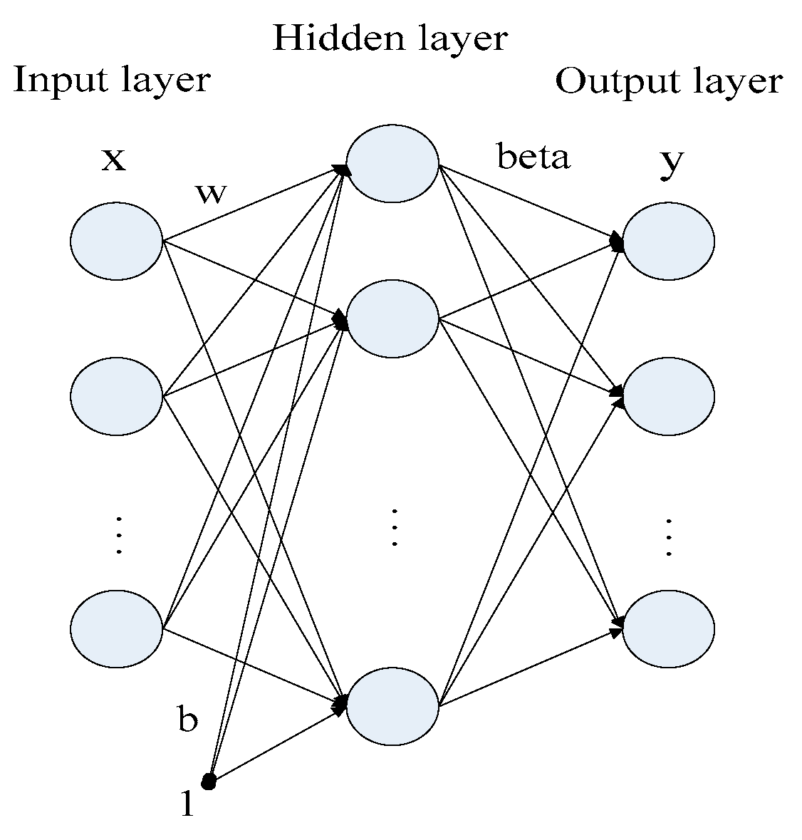
Huang et al. [31] put forward the extreme learning machine (ELM) model in 2004, which has a higher precision of generalization as well as a faster convergence speed than the abovementioned models. Moreover, it can avoid many of the problems that may arise in gradient-based learning methods; for instance, stopping criteria and learning periods. As a consequence, it has been widely employed to make predictions in a variety of fields since its introduction. Shrivastava and Panigrahi [32] investigated the performance of a combination of ELM and the Wavelet technique (WELM) in price forecasting in electricity markets. The empirical research demonstrated that this model is appropriate for price forecasting. Liu et al. [33] applied the ELM model in wind speed forecasting. In this study, the ARIMA model and the SVM model were involved in a comparison of the prediction performance. The experimental results showed that the proposed WPD-EMD-ELM model performed the best among the compared models. Furthermore, an ELM’s input weights matrix and hidden layer bias are key parameters in the ELM’s generalization capability. Based on this, it is essential to utilize an optimization algorithm to obtain the optimal parameters. Rocha et al. 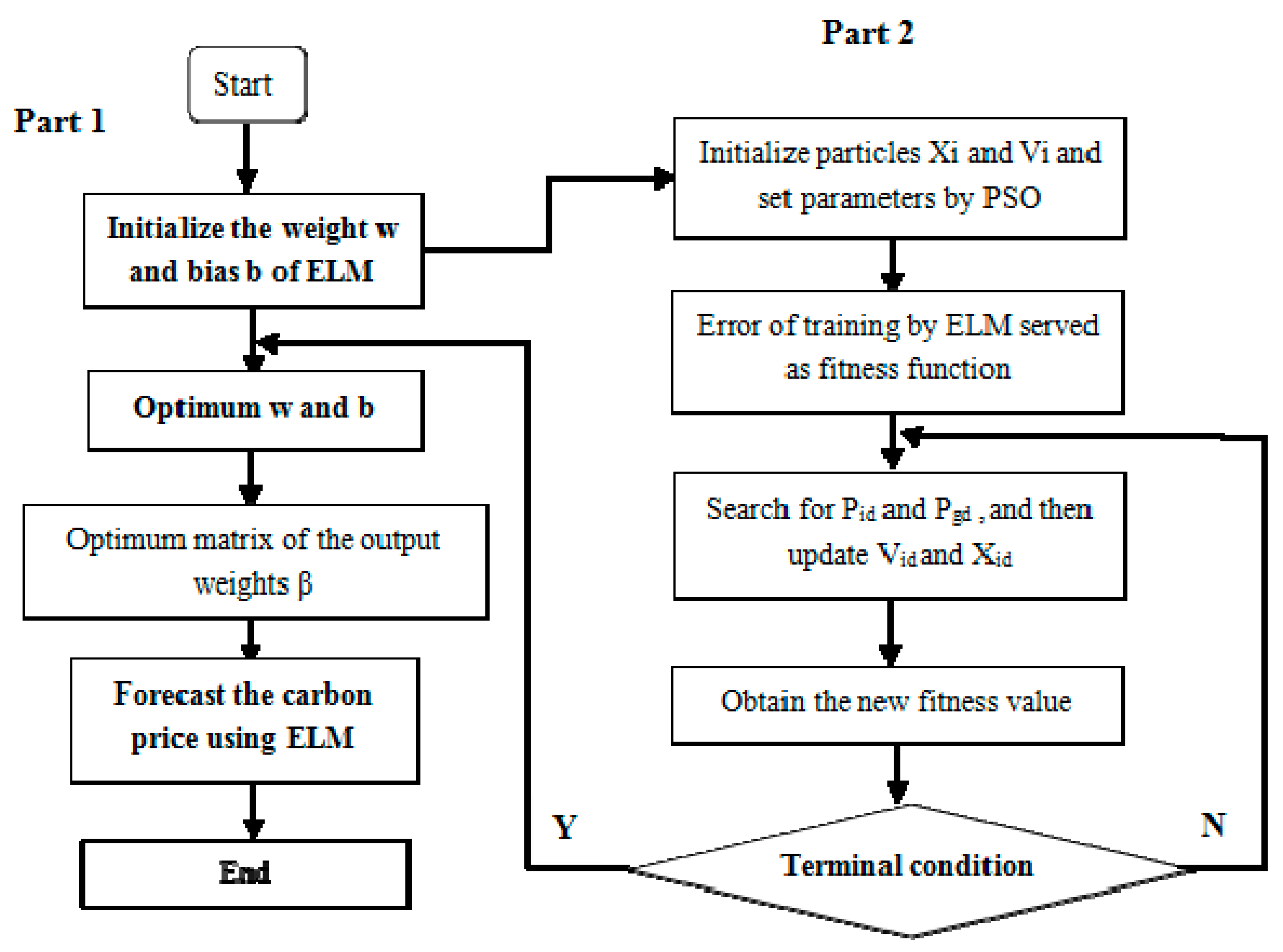[34] implemented parameter selection for an ELM improved by Particle Swarm Optimization (PSO-ELM) in the forecasting of a distributed electrical generation system’s capacity. Fan et al. [35] proposed a PSO-ELM model for short-term power load forecasting. The results proved that the improved model showed a higher learning rate and prediction accuracy compared with the traditional ELM model. From the above, it can be found that the ELM-type models have been well-employed in a variety of forecasting scenarios. Therefore, one of the purposes of this paper is to verify the feasibility of the PSO-ELM model for carbon price prediction.

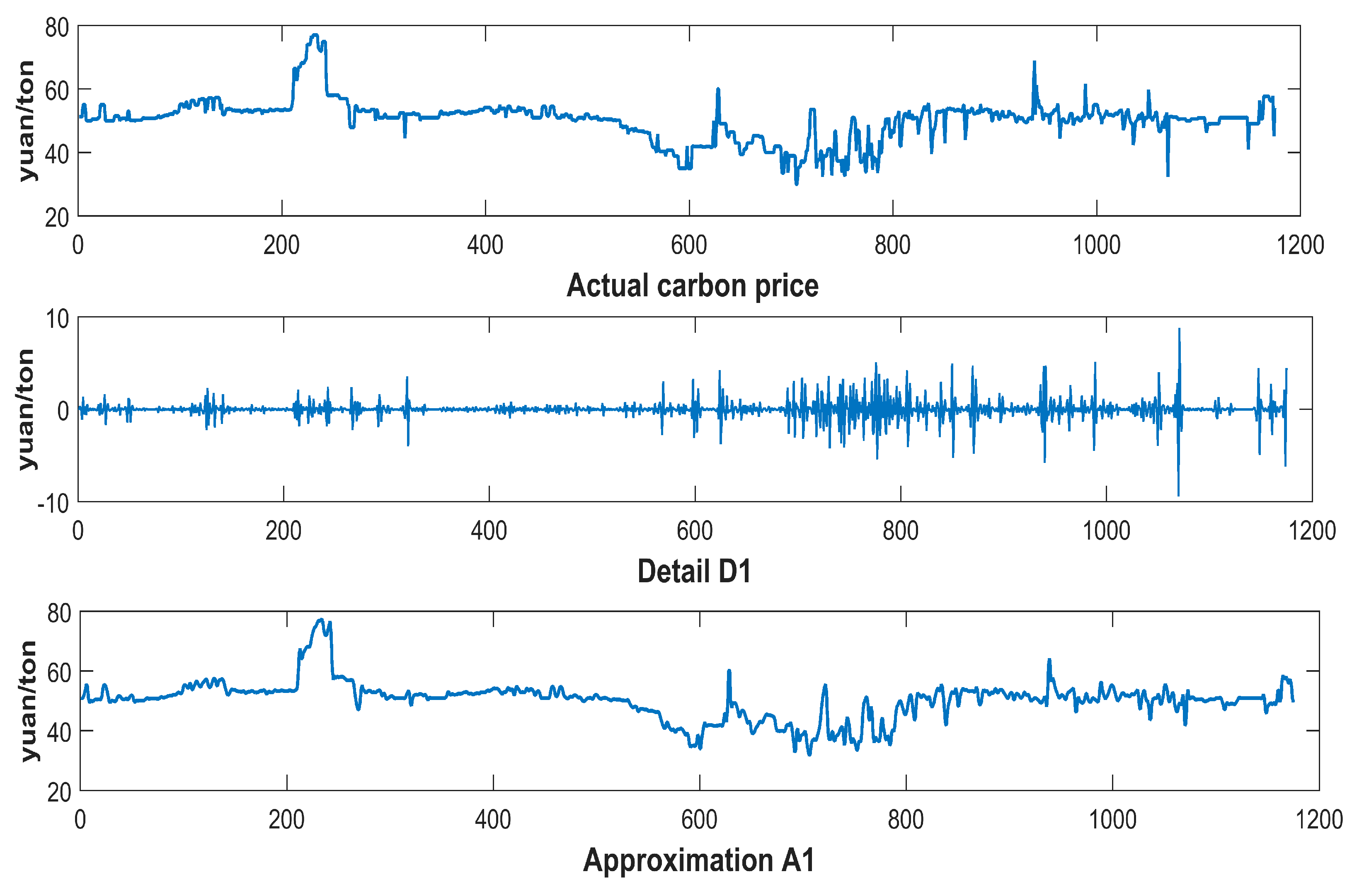
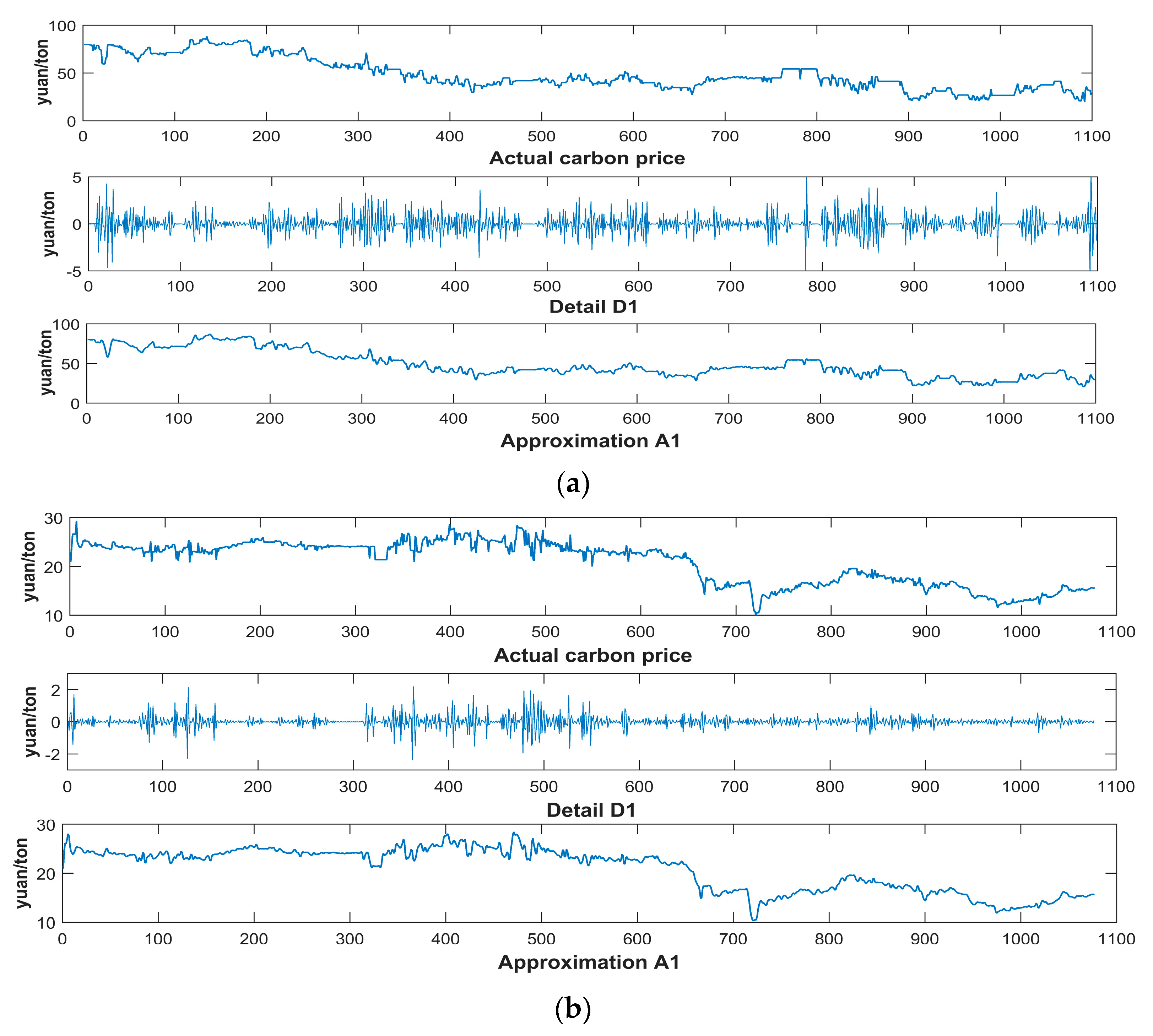
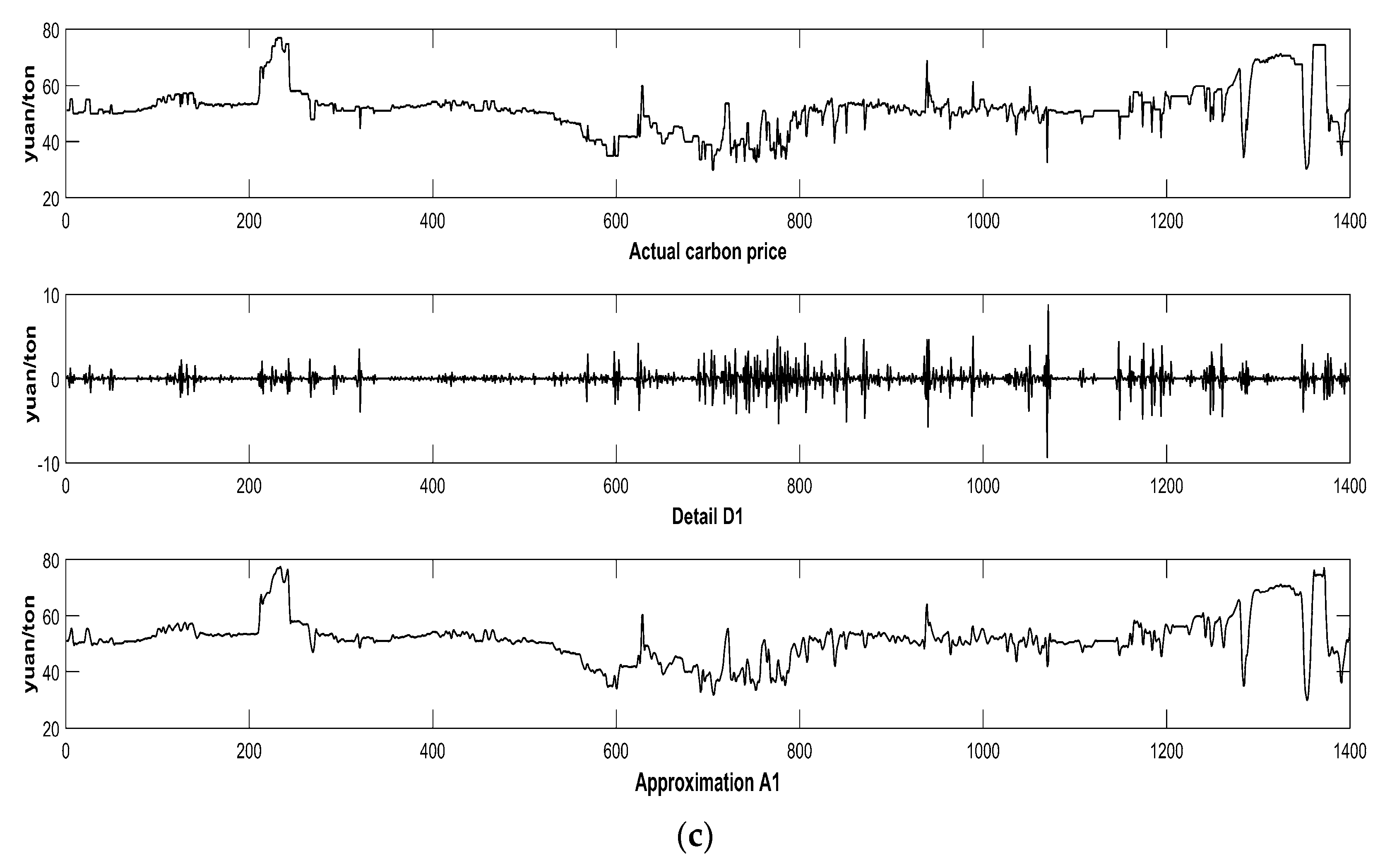
Given the chaotic property and intrinsic complexity of carbon prices, it may not be appropriate to directly forecast carbon prices before data preprocessing. Presently, empirical mode decomposition (EMD) and the wavelet transform (WT) are considered to be the common data preprocessing approaches for decomposing the initial series and eliminating the random volatility. WT was applied to signal processing in electricity market price forecasting by Saber et al. [36]. In the process of analyzing the unified interval price of China’s carbon trading market, Li and Lu [37] applied the GARCH-EMD model to predict carbon prices. The results demonstrate that EMD is an effective method to decompose unstable carbon prices. Zhu et al. 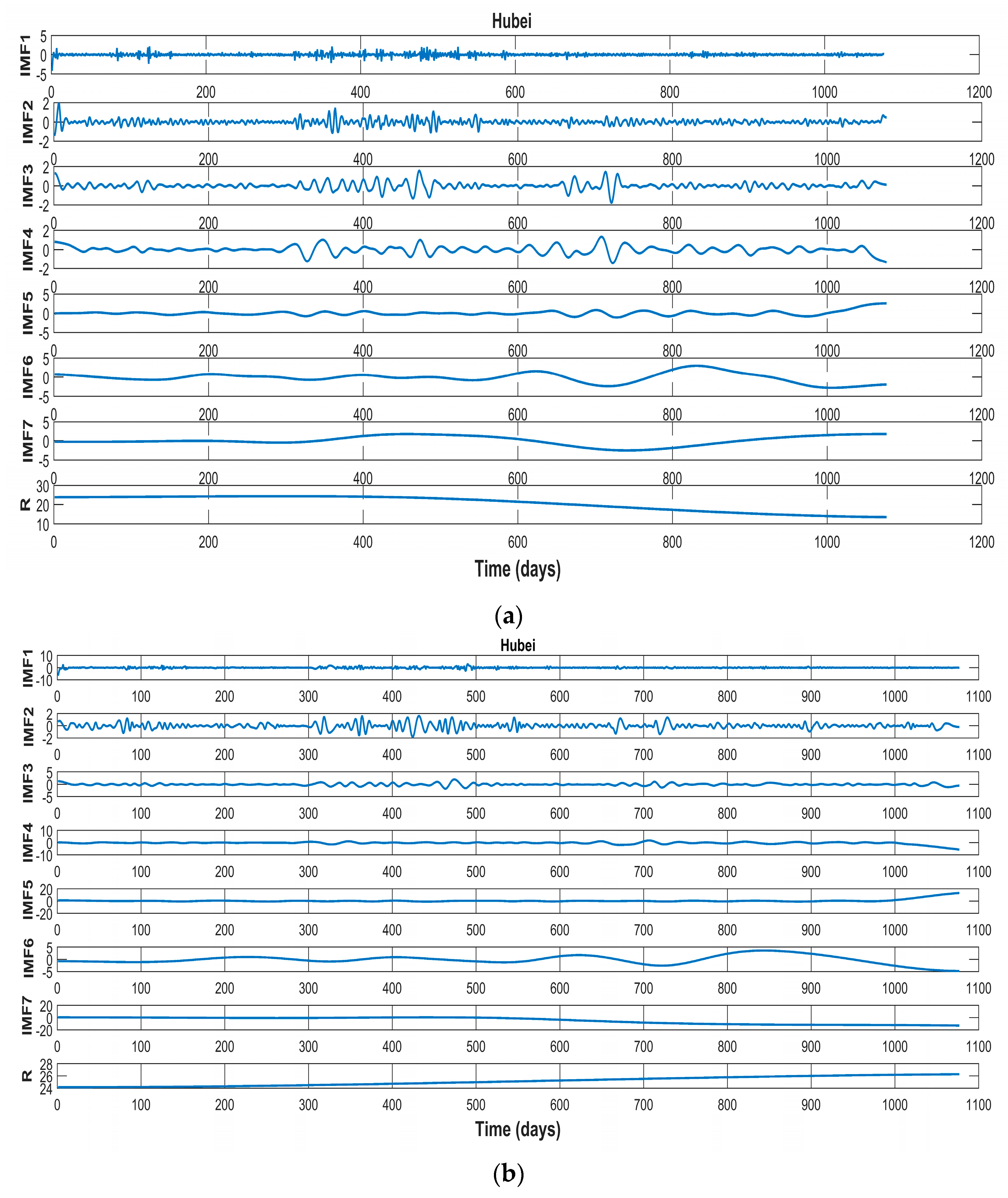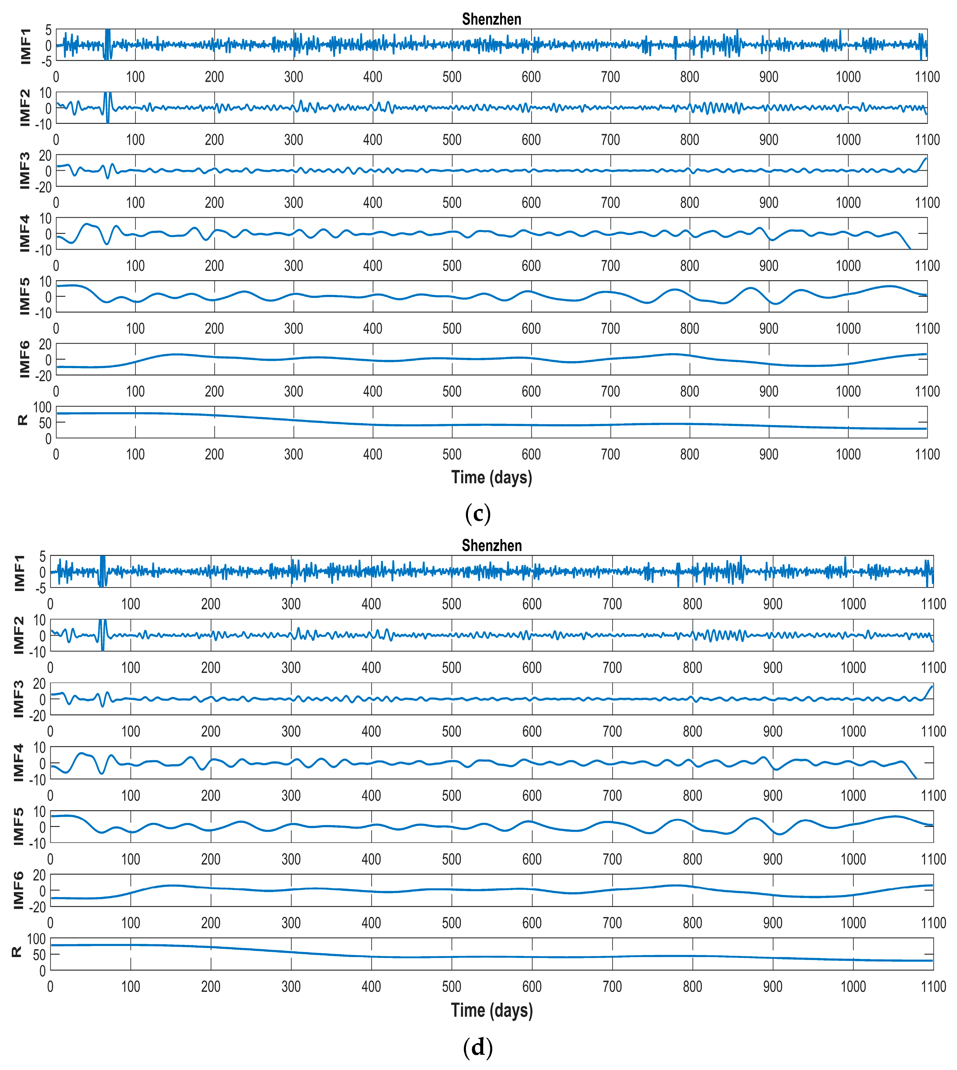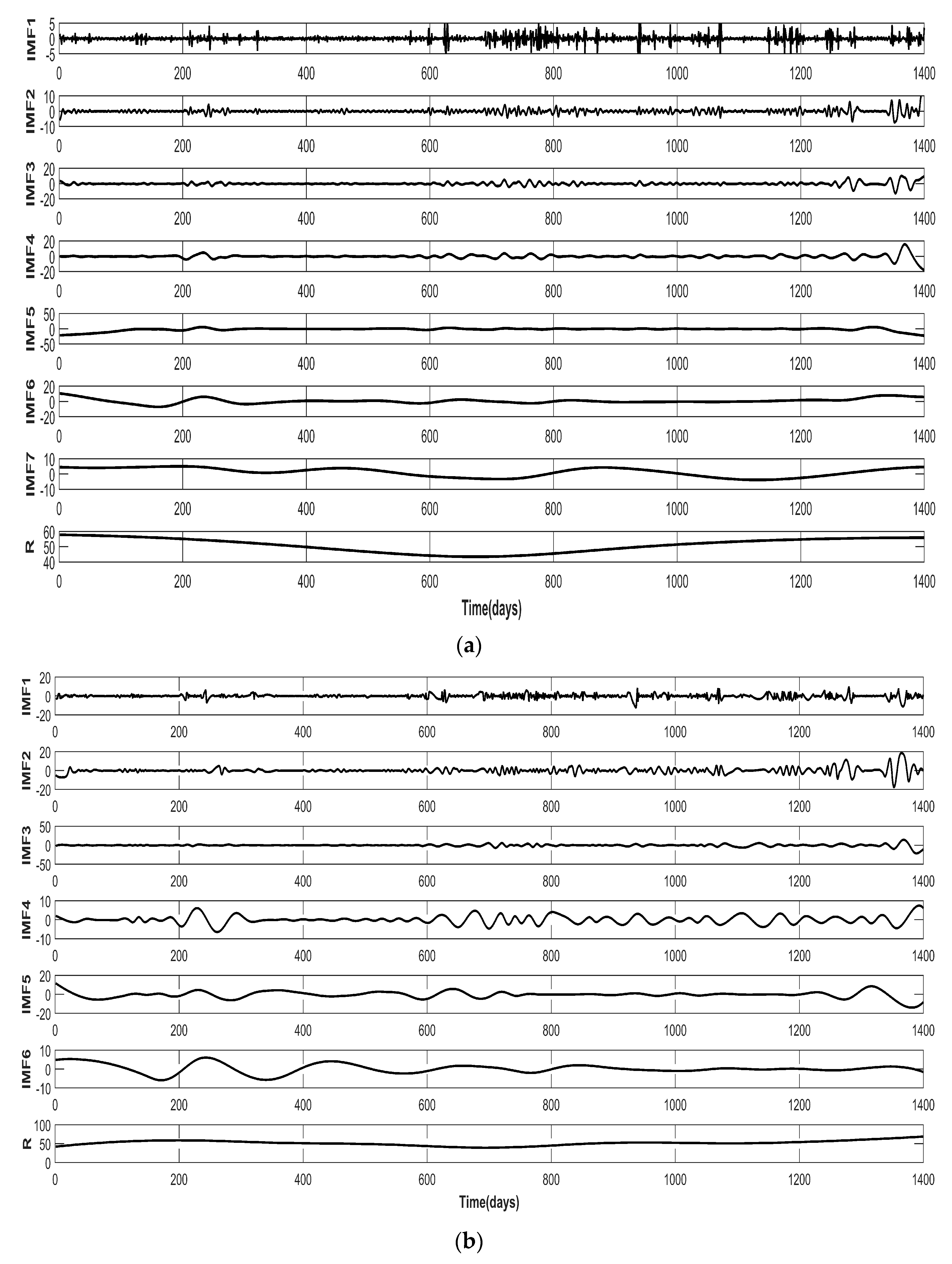[38] built a multiscale model that combined EMD and developmental least squares support vector regression (LSSVR) for carbon price forecasting with a high accuracy. Basing on the data from the E.U. ETS, the empirical results showed that the EMD-LSSVR model performed the best in comparison with other prediction models according to the values of statistical indicators. It is worth noting that EMD may have a mode mixing problem that causes the decomposed intrinsic mode functions (IMFs) to lose their meaning. To tackle the problem, Huang and Wu carried out ensemble empirical mode decomposition (EEMD) via introducing white noise into the original series [39]. In 2014, fast ensemble empirical mode decomposition (FEEMD) was proposed to improve EEMD’s computing capacity for a large amount of sample data [40]. They were all used successfully in wind speed forecasting. Heng et al. [41] reconstructed the initial data for wind speed forecasting by FEEMD. 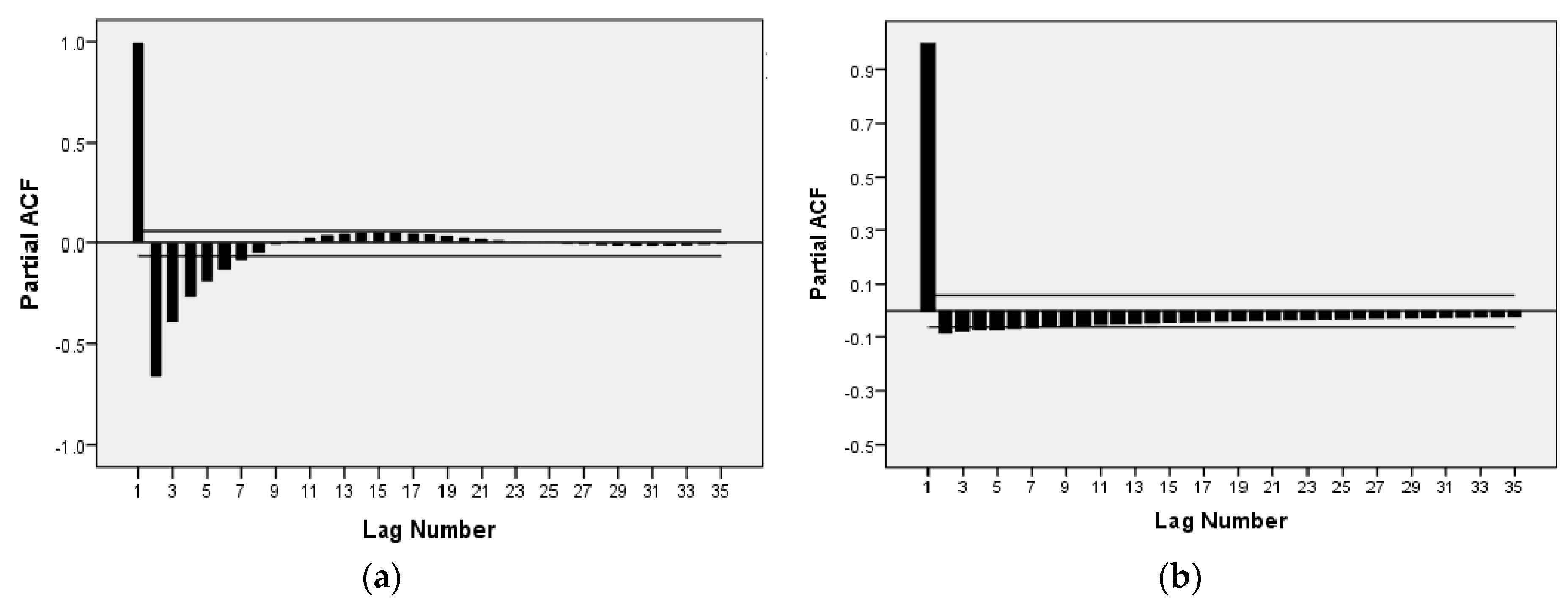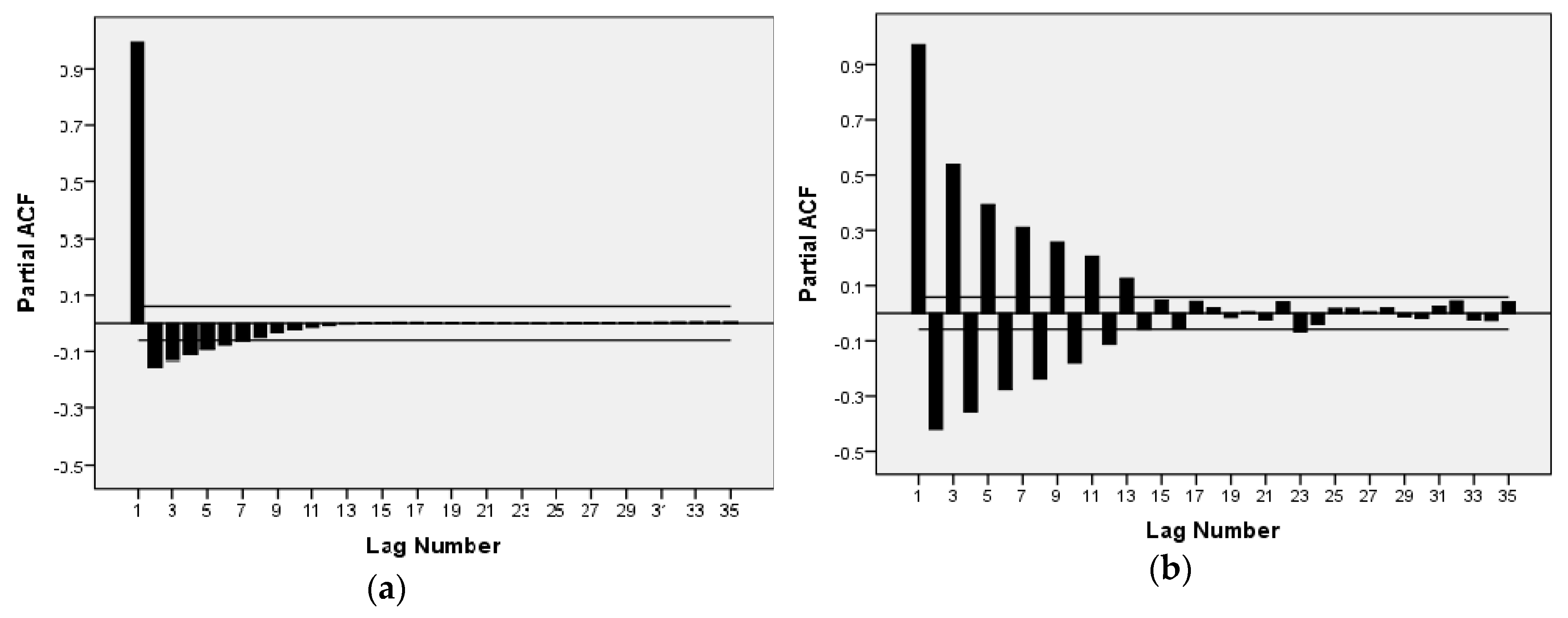Sun and Liu proposed EMD and FEEMD for processing the original wind speed data, and then combined these methods with different intelligent algorithms for the prediction of wind speed [42,43]. Thanks to carbon prices having dynamic and nonlinear properties that are similar to those of wind speed, this paper proposes EMD and FEEMD to decompose a carbon price series and introduces both a phase space reconstruction theory (PSR) and a partial autocorrelation function (PACF) for the analysis of the decomposed subsequences.

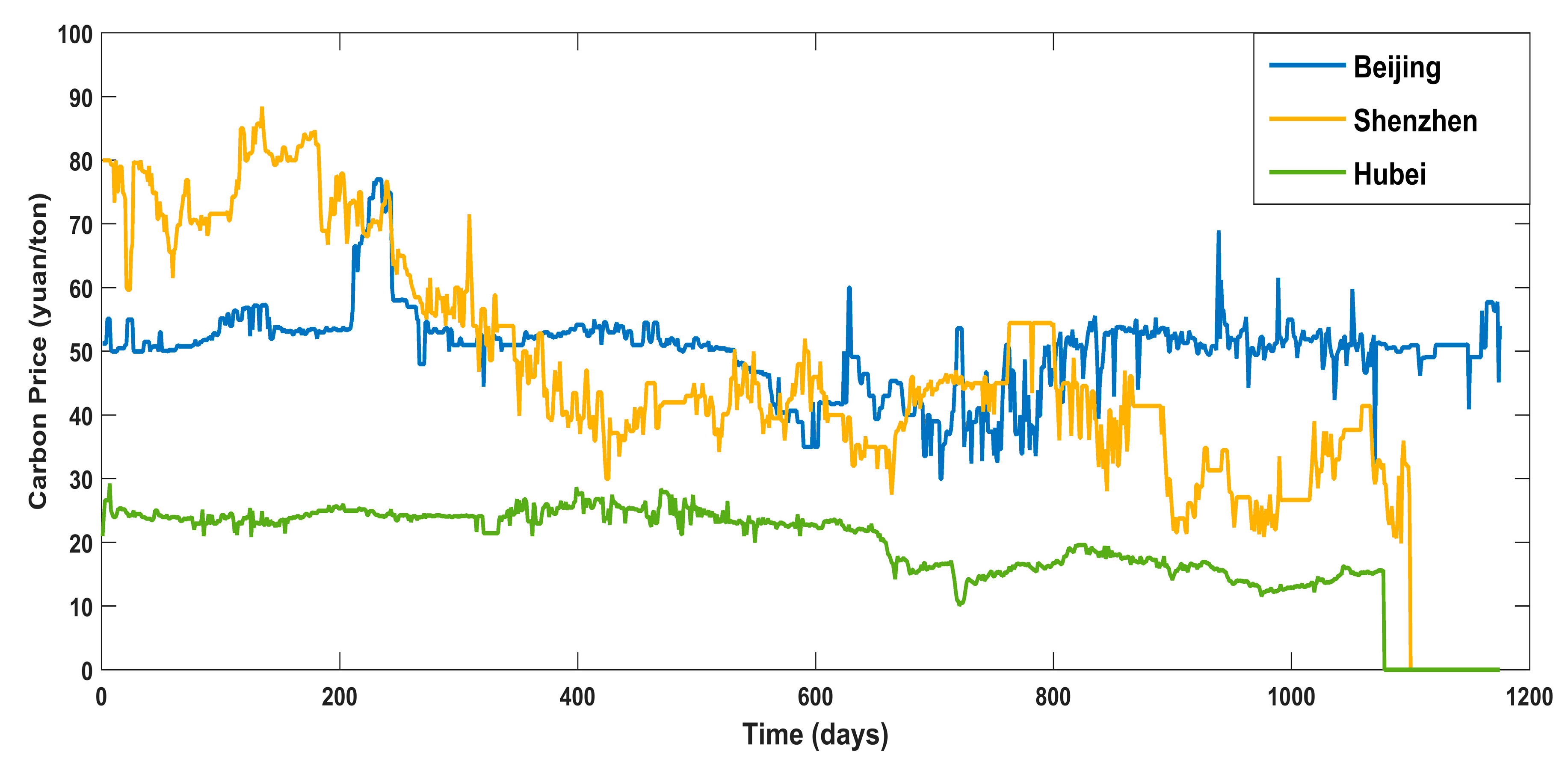
Currently, China has constructed eight regional carbon markets, and, on 19 December 2017, started the construction of the national carbon market. As the earliest pilot markets, the Beijing, Shenzhen, and Hubei carbon markets have been in smooth operation and gradually formed their features in the process of promoting emission reductions.

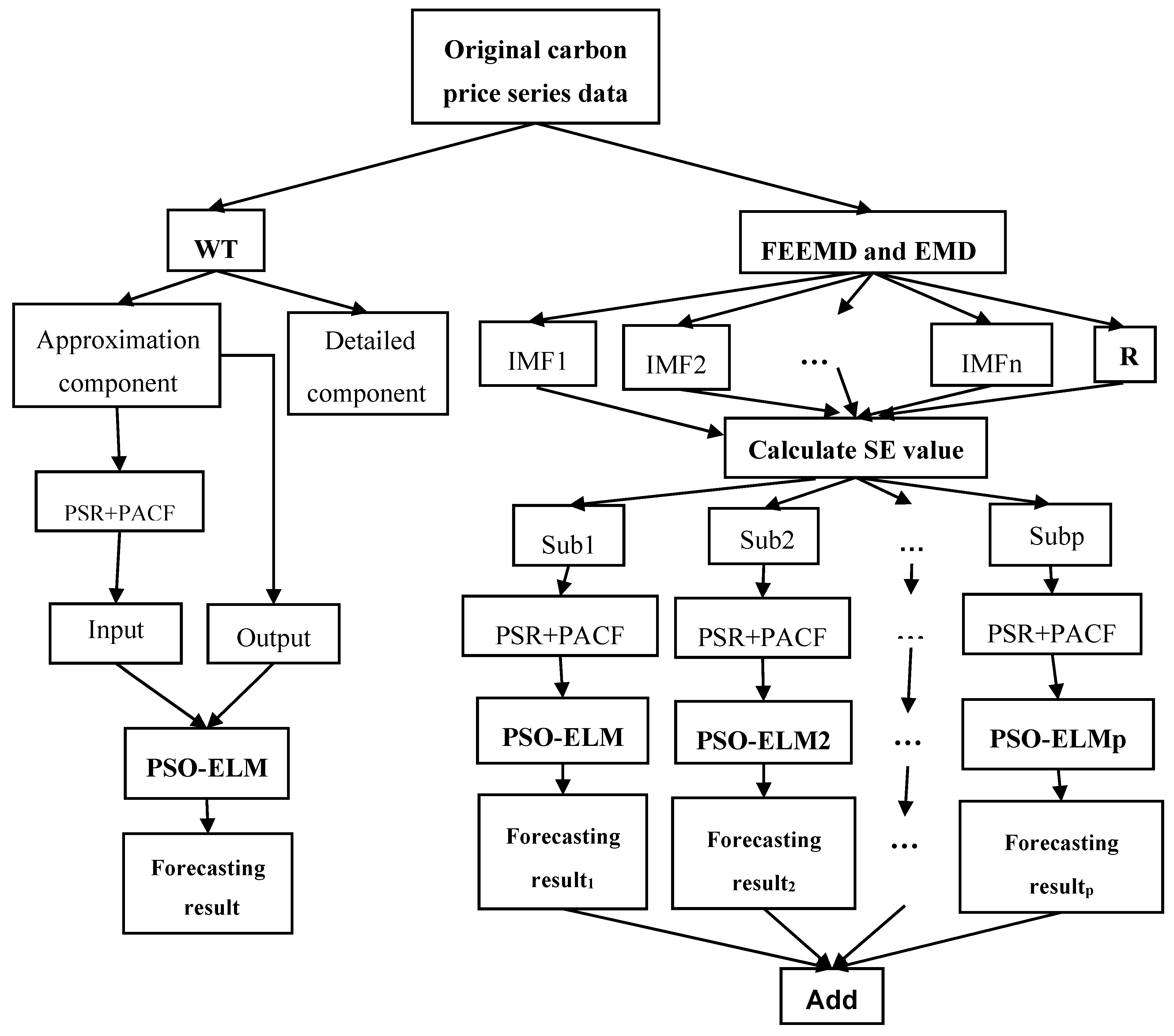
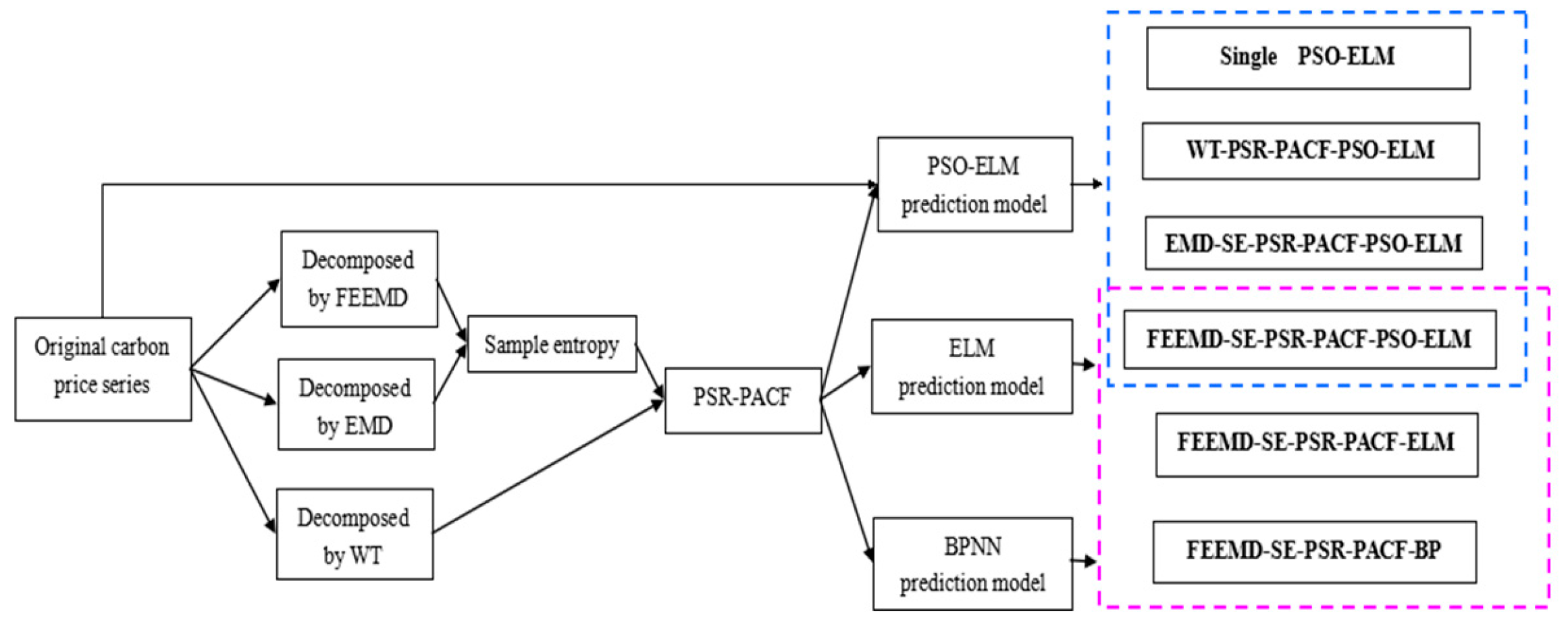
Having summarized the research of our predecessors, this thesis selects the carbon price of Beijing, Shenzhen, and Hubei as the example. We focus on Beijing’s carbon price, and analyze the features through a comparison with the other two typical markets. After being decomposed by the FEEMD, the IMFs are analyzed by phase space reconstruction and a partial autocorrelation function to determine the input of the forecasting models in the next step. Additionally, this paper adopts the PSO-ELM model to forecast carbon prices.

The main contribution of this paper is this new hybrid combination model for carbon price prediction, which is expressed as FEEMD-PSR-PACF-PSO-ELM. Firstly, this paper comprehensively considers the chaotic property and the partial autocorrelation of decomposed carbon price subsequences to reconstruct the input and output variables. Secondly, the research idea, which is based on the FEEMD model combined with the PSO-ELM model to decompose carbon prices, represents a new attempt to predict carbon prices.

The rest of this paper is divided into four sections. Section 2 presents the methods and models that are applied in this paper, including the decomposition methods, the chaotic series reconstruction, and the hybrid prediction model. An exhaustive explanation of the hybrid forecasting models that are proposed in this paper is given in Section 3. The data processing and the analysis of carbon price forecasting based on actual data from different regions under China’s ETS are presented in Section 4. Finally, Section 5 provides conclusions according to the results of the empirical analysis.

2. Materials and Methods

2.1. The Particle Swarm Optimization Algorithm

Proposed by Kennedy and Eberhart [44] in 1995, the particle swarm optimization algorithm simulates bird predation behavior and calls each bird a particle. As a well-recognized optimization algorithm, its rationale is to continuously update the distance between P_best (the best location found by itself) and G_best (the current global best position). Suppose that, in a D-dimensional search space, the t-th particle is presented by X_t = (x_t1, x_t2, …, x_tD)^T, and the speed and the P_best are expressed as V_t = (v_t1, v_t2, …, v_tD)^T and P_t = (p_t1, p_t2, …, p_tD)^T, respectively. In addition, G_best is stated as G_t = (G_t1, G_t2, …, G_tD). A kernel of PSO can be expressed as:

$$V_{td}^{k+1}=w{V}_{td}^k+c_1{r}_1(P_{td}^k-X_{td}^k)+c_2{r}_2(G_{td}^k-X_{td}^k)$$

(1)

$$X_{td}^{k+1}=X_{td}^k+V_{k+1td},d=1,2,\dots ,D;k=1,2,\dots ,n$$

(2)

where w is assumed to be the inertia weight to amend the search range, and c₁ and c₂ are acceleration factors set to 1.4945. Afterwards, r₁ and r₂ are assigned evenly among the interval [0, 1]. In order not to blindly search, the position and speed values have limitations of [−X_max, X_max] and [−V_max, V_max], respectively.

2.2. Extreme Learning Machine

Extreme learning machine is an innovative algorithm based on a feed forward neural network as shown in Figure 1. The gradient descent algorithm is used to regulate the weights and parameters in the training process. Meanwhile, the Moore–Penrose inverse is used to calculate the hidden layer matrix to transform the training process into a solution to a least square problem. ELM has a faster learning velocity in comparison with other neural network models, and it can be used for classification, regression, clustering, and sparse approximation while guaranteeing learning accuracy at the same time.

Of note is that, during the learning process, the weight values and thresholds may have non-optimal values, which lead to poor performance and an unstable output. Actually, ELM needs a large number of hidden layer nodes to reach an expected result, which may make it prone to overfitting. To resolve these problems, this paper uses PSO to optimize the deviation of the hidden layer and the input layer weight of ELM, referred to as PSO-ELM, which works as shown in Figure 2. In Figure 2, Part 1 is the forecasting process of the extreme learning machine, and Part 2 is the principle of the particle swarm optimization algorithm. The proposed model not only takes full advantage of PSO’s global search capability and ELM’s rapid convergence rate, but also overcomes the inherent problems of ELM.

2.3. Fast Ensemble Empirical Mode Decomposition and Sample Entropy

As described above, fast ensemble empirical mode decomposition (FEEMD) is a fast implementation of EEMD. It is often used for signal decomposition, which decomposes a nonstationary timing signal X(i) (i = 1, 2, …, n) into a finite number of IMFs and one residual R component. Moreover, it can effectively solve the mixing mode phenomenon of EMD, and introduces white noise and the idea of an ensemble average. Given the features of a dataset, the amplitude k of white noise is set as 0.05–0.5 times and the iteration time M is set to 100.

Sample entropy (SE) is a modification of approximate entropy (AE), which is used to assess the complexity of physiological time-series signals, diagnose disease states, and so on, and was proposed in 2000 by Richman et al. [45]. The larger the SE values, the higher the sample complexity. Furthermore, SE has two advantages over AE: data length independence and better consistency; that is, the influence of the parameters on the sample entropy is the same. The SE value has three important parameters, denoted by N, m, and r, where N expresses the length of subsequences, m represents the dimension, and r is the similarity tolerance. The formula for calculating SE is shown below.

$$\mathrm{SE}=\underset{\mathrm{N}\to \infty }{\lim }\{-\ln [{\mathrm{B}}^{\mathrm{m}+1}(\mathrm{r})/{\mathrm{B}}^{\mathrm{m}}(\mathrm{r})]\}$$

(3)

Since N cannot be an infinite value in an actual calculation application, N takes a finite value, and the sample entropy is calculated as:

$${\mathrm{SE}(\mathrm{N},\mathrm{m},\mathrm{r})=-\ln [\mathrm{B}}^{\mathrm{m}+1}{\left(\mathrm{r}\right)/\mathrm{B}}^{\mathrm{m}}\left(\mathrm{r}\right)]$$

(4)

Generally, in practical applications, m is 1 or 2, and r is set from 0.1 × std to 0.25 × std (where std represents the original sequences’ standard deviation). Therefore, this paper sets m at 2 and r as 0.2 × std. Based on the characteristics of the SE value, this paper judges the autocorrelation of each decomposed sequence by calculating the SE value, and then combines the sequences with similar SE values. In other words, sequences with similar complexity are combined into new sequences to prepare for follow-ups.

2.4. Phase Space Reconstruction and the Maximal Lyapunov Exponent

Phase space reconstruction was put forward to deal with the complexity and nonlinearity in time series based on Chaos. Considering the nonlinear and chaotic characteristics of carbon price time series, this paper applied phase space reconstruction (PSR) to reconstruct the phase space of each subsequence to accurately determine the input of carbon price prediction. In general, regarding a time series {x_i} = {x₁, x₂, …, x_N} with τ (the delay time) and m (the embedded dimension), which are two key parameters of PSR, the reconstructed matrix is calculated by:

$$X(k)=[x(k),x(k+\tau ),\cdots ,x(k+(m-1)\tau )].$$

(5)

Then, the original time series and the corresponding output can be reconstructed as:

$$\begin{array}{l}\left[\begin{array}{c}{X}_1\\ X_2\\ ⋮\\ X_{N-m+1}\end{array}\right]=\left[\begin{array}{cccc}x(1)& x(1+\tau )& \cdots & x(1+(m-1)\tau )\\ x(2)& x(2+\tau )& \cdots & x(2+(m-1)\tau )\\ ⋮& ⋮& \ddots & ⋮\\ x(N-m+1)& x(N-m+1+\tau )& \cdots & x(N-m+1+(m-1)\tau )\end{array}\right]\end{array}$$

(6)

$$\left[\begin{array}{c}x(2+(m-1)\tau )\\ x(3+(m-1)\tau )\\ ⋮\\ x(N)\\ x(N+1)\end{array}\right].$$

(7)

In mathematics, the Lyapunov index of a dynamic system describes the properties of the separation rate of infinitely small close tracks [46]. Whether the system has dynamic chaos can be judged intuitively from whether the maximum Lyapunov exponent is greater than zero: a positive Lyapunov exponent means that, no matter how small the spacing between the initial two trajectories is, the difference will increase exponentially with time in the system’s phase space, so that it can be called Chaos. There are many ways to calculate the maximal Lyapunov exponent, such as the Wolf method and Gram–Schmidt Renormalization. This paper uses the widely used method ‘Wolf’ [47] to calculate the maximal Lyapunov exponent under PSR.

3. The Framework of the Proposed Model

Figure 2 displays the flowchart of the proposed PSO-ELM model for carbon price prediction. Part 1 is the calculation process of the PSO algorithm and Part 2 is the forecasting procedure of ELM. In a word, this paper utilizes PSO to optimize the key parameters of ELM.

The focus of the overall hybrid model in this paper can be divided into two parts, which are presented in Figure 3. One part is to decompose the initial carbon price time series to determine the input and output of the prediction model. The other part is to forecast the carbon price and verify the accuracy of the proposed prediction model.

This paper utilizes FEEMD, EMD, and WT for the decomposition of a carbon price series. For FEEMD and EMD, the original data is decomposed into several IMFs. Then, this paper calculates the SE value of each IMF separately to judge its complexity, and the IMFs with similar SE values are merged to form several new subsequences. PSR is performed for each subsequence, and the maximum Lyapunov exponent is calculated to test the chaotic characteristics of each subsequence. In particular, this paper uses PACF to analyze those subsequences whose chaotic characteristics are not significant. In this way, after comprehensively analyzing the characteristics of the sequences, the input and output of the PSO-ELM model can be determined more reasonably. Similarly, in part two, after WT decomposition, the initial data is transformed into an approximate sequence and a detailed sequence. The detailed sequence is discarded. Then, the same steps of part one are followed to perform phase space reconstruction and a partial autocorrelation analysis to determine the input and output of PSO-ELM. The forecasting is divided into training sets and test sets. Finally, the forecast is compared with the actual carbon price.

4. Empirical Analysis

4.1. Data

As the capital of China, Beijing’s carbon market development is related to the sustainable development of the capital in the future. The Beijing carbon market mechanism provides basic support to the strategic positioning of the capital’s “four centers”. In addition, we select the carbon price data from the Shenzhen and Hubei carbon markets to perform a comparative analysis. The Shenzhen and Hubei carbon markets are typical carbon markets in China with a longer transaction time and a higher transaction volume. Afterward, we chose the daily transaction price of these three carbon markets for empirical studies. The training set and testing set were divided according to a ratio of 7:3.

We selected the carbon price of the Beijing carbon market from 28 November 2013 to 29 December 2017 in the first case study to verify the hybrid model’s applicability. The carbon price data from the Shenzhen carbon market from 1 November 2013 to 29 December 2017 and the data from the Hubei carbon market from 2 April 2014 to 20 June 2017 were used to further test the model’s validity. To further validate the effectiveness of the model, we updated the latest data on the Beijing carbon market and conducted an empirical analysis as shown in Section 4.4. Figure 4 shows the original price data from these three regional carbon markets, which were obtained from the literature and an official website with the address: http://www.tanjiaoyi.com/.

4.2. Case Study of the Beijing Carbon Price

4.2.1. Carbon Price Decomposition

It can be seen from Figure 4 that the original carbon price series of the regional carbon markets all have serious fluctuations. In order to reduce noise interference, this paper proposes the FEEMD method to decompose carbon prices. At the same time, EMD and WT were also employed to decompose the same Beijing carbon price series so as to test the superiority of FEEMD. The results are shown in Figure 5 and Figure 6, respectively. Figure 5a expresses that the FEEMD decomposed the Beijing carbon price series into seven IMFs and one remainder; Figure 5b shows that EMD decomposes the series into six IMFs and one remainder. In Figure 6, the original data were decomposed into an approximation A1 and a detail D1 by WT. A1 was expected to present the main fluctuation, while D1 depicted the highest frequency. Therefore, A1 was used for prediction in this paper.

4.2.2. The Calculation of Sample Entropy

As described above, SE is used to measure the complexity in a series. Since decomposition by FEEMD and EMD results in a large number of IMFs, this paper calculates the SE values of each IMF, which are shown in

Table 1. The results on the sample entropy (SE) values.

Sub		IMF1	IMF2	IMF3	IMF4	IMF5	IMF6	IMF7	IMF8
SE Value	Processed by FEEMD	0.7972	0.4772	0.3983	0.3557	0.0849	0.0649	0.0246	0.0073
	Processed by EMD	0.595	0.3777	0.1908	0.0222	0.0269	0.0326	0.0079

and Figure 7, so as to understand their complexity and merge them into new sequences, which will improve the computational efficiency. The recombination results are exhibited in

Table 2. The new subsequence after being processed by fast ensemble empirical mode decomposition (FEEMD).

Index	Sub1	Sub2	Sub3	Sub4	Sub5
Results	IMF1	IMF2	IMF3, IMF4	IMF5, IMF6	IMF7, R

and

Table 3. The new subsequence after being processed by empirical mode decomposition (EMD­).

Index	Sub1	Sub2	Sub3	Sub4
Results	IMF1	IMF2	IMF3	IMF4, IMF5, IMF6, R

. The new subsequences will be used in the carbon price predictions.

4.2.3. Input and Output Selection

In the process of predicting each subsequence, the key part is the determination of the input and output. This paper introduces phase space reconstruction and the PACF method to reconstruct the subsequences.

Firstly, after calculation of the τ and m for each subsequence, the phase space is rebuilt based on Formulas (6) and (7). At the same time, the maximal Lyapunov exponents are calculated to examine the chaotic properties. After obtaining the τ and m of the five series after decomposition by FEEMD, the answers can be seen in

Table 4. The parameters of each subsequence after processing by FEEMD-SE.

Index	Sub1	Sub2	Sub3	Sub4	Sub5
τ	2	2	6	18	5
m	13	24	15	14	4
Max Lyapunov index	1.689	0.03	0.128	−166.2	−169.7
Train	X1–X806	X1–X791	X1–X763	(xi−1, xi−2, xi−3, xi−4, xi−5, xi−6, xi−7) (size: 818)	(xi−1, xi−2) (size: 821)
Test	X807–X1150	X792–X1128	X764–X1090	(xi−1, xi−2, xi−3, xi−4, xi−5, xi−6, xi−7) (size: 350)	(xi−1, xi−2) (size: 352)

.

Secondly, there may be non-chaotic subsequences. This paper introduces a PACF analysis on these subsequences to make the determination of the input and output more complete and reasonable. In a word, the main idea of PACF is to find the lags that satisfy the 95% confidence interval.

In Table 4, we found that the maximal Lyapunov exponents of sub4 and sub5 are negative. Theoretically speaking, these subsequences do not have chaotic characteristics; so, phase space reconstruction methods are not suitable for them. Therefore, we used the PACF method to analyze sub4 and sub5. The results are shown in Figure 8, and the Train and Test sets are shown in Table 4. For instance, sub5 was reconstructed using PACF and two lags were obtained, and the size of the data in the Train and Test sets was set according to the ratio of 7 to 3. Similarly,

Table 5. The parameters of each subsequence after processing by EMD-SE.

Index	Sub1	Sub2	Sub3	Sub4
τ	9	10	6	14
m	15	11	15	7
Max Lyapunov index	1.38	0.512	0.029	−167.6
Train	X1–X733	X1–X751	X1–X763	(xi−1, xi−2, xi−3, xi−4, xi−5, xi−6) (size: 818)
Test	X734–X1048	X753–X1074	X764–X1090	(xi−1, xi−2, xi−3, xi−4, xi−5, xi−6) (size: 351)

and Figure 9a show the results of the PSR and PACF analysis of the subsequences decomposed by EMD, respectively. In addition, we found that, through the result on its maximal Lyapunov exponent, which is shown in

Table 6. The parameters of the approximation subsequences decomposed by wavelet transform (WT).

Index	Beijing	Shenzhen	Hubei
τ	7	7	5
m	20	14	21
Max Lyapunov index value	−165.36	−165.05	−165.32
Train	(xi−1, xi−2, xi−3, xi−4, xi−5, xi−6, xi−7, xi−8, xi−9, xi−10, xi−11, xi−12, xi−13) (size: 814)	(xi−1, xi−2, xi−3, xi−5) (size: 766)	(xi−1, xi−2, xi−3, xi−4, xi−5, xi−6) (size: 750)
Test	(xi−1, xi−2, xi−3, xi−4, xi−5, xi−6, xi−7, xi−8, xi−9, xi−10, xi−11, xi−12, xi−13) (size: 349)	(xi−1, xi−2, xi−3, xi−5) (size: 328)	(xi−1, xi−2, xi−3, xi−4, xi−5, xi−6) (size: 321)

, the approximation (A1) component decomposed by WT did not satisfy the chaotic characteristic. Figure 9b shows the PACF analysis result of A1. In order to clearly understand the meaning of Figure 8 and Figure 9,

Table 7. The coefficients of different subsequences processed by partial autocorrelation function (PACF).

Lag	Std. Error	Partial Autocorrelation Coefficients of Subs
		Sub4 after FEEMD	Sub5 after FEEMD	Sub4 after EMD	Sub after WT
1	0.029	0.998	1	0.995	0.972
2	0.029	−0.67	−0.085	−0.154	−0.421
3	0.029	−0.394	−0.078	−0.131	0.538
4	0.029	−0.268	−0.073	−0.111	−0.357
5	0.029	−0.189	−0.068	−0.093	0.393
6	0.029	−0.131	−0.064	−0.076	−0.276
7	0.029	−0.085	−0.06	−0.061	0.31
8	0.029	−0.047	−0.057	−0.047	−0.238
9	0.029	−0.016	−0.054	−0.035	0.257
10	0.029	0.009	−0.051	−0.024	−0.18
11	0.029	0.028	−0.049	−0.016	0.206
12	0.029	0.041	−0.046	−0.009	−0.112
13	0.029	0.049	−0.044	−0.003	0.126
14	0.029	0.054	−0.042	0	−0.058
15	0.029	0.055	−0.041	0.003	0.047
16	0.029	0.053	−0.039	0.004	−0.056
17	0.029	0.049	−0.038	0.004	0.043
18	0.029	0.044	−0.036	0.003	0.02
19	0.029	0.037	−0.035	0.002	−0.015
20	0.029	0.03	−0.034	0.001	0.005
21	0.029	0.022	−0.032	0	−0.024
22	0.029	0.015	−0.031	0	0.041
23	0.029	0.007	−0.03	−0.001	−0.067
24	0.029	0	−0.029	−0.001	−0.04
25	0.029	−0.006	−0.028	0	0.017
26	0.029	−0.011	−0.027	0	0.018
27	0.029	−0.016	−0.026	0.001	0.006
28	0.029	−0.019	−0.026	0.002	0.019
29	0.029	−0.021	−0.025	0.003	−0.013
30	0.029	−0.022	−0.024	0.004	−0.018
31	0.029	−0.022	−0.023	0.005	0.025
32	0.029	−0.021	−0.022	0.005	0.044
33	0.029	−0.019	−0.022	0.006	−0.024
34	0.029	−0.017	−0.021	0.006	−0.026
35	0.029	−0.014	−0.02	0.006	0.041

lists the autocorrelation coefficients of each subsequence after PACF. With the data in Table 7, it can be seen that the coefficients of the lags that exceed the limit range line in Figure 8 and Figure 9 are two times greater than the standard error; so, we extract them as significant lags for prediction.

4.2.4. Forecasting Evaluation Criteria

In order to effectively evaluate the performance of the prediction models, this paper selected the root mean square error (RMSE) and the mean absolute percentage error (MAPE) to test the accuracy of the proposed models. As general error indicators, we know that the larger the value, the worse the performance and vice versa. The formulas are listed as follow.

$$RMSE=\sqrt{\frac{1}{n}{\displaystyle \sum _{t=1}^n{\left|\frac{{\widehat{y}}_t-y_t}{y_t}\right|}^2}}$$

(8)

$$MAPE=\frac{1}{n}{\displaystyle \sum _{t=1}^n\left|\frac{{\widehat{y}}_t-y_t}{y_t}\right|}*100\%$$

(9)

where n represents the amount of data in the test set, $y_t$ is the t-th actual data, and ${\widehat{y}}_t$ is the matching prediction output.

4.2.5. Beijing Carbon Price Forecasting

First of all, to show the forecasting performance capability of this hybrid model, the models for the comparison are established as shown in Figure 10. Figure 10 is divided into two main parts. The first part compares the influence of different decomposition methods, which are shown in the blue box. The second part emphasizes the forecasting veracity among the prediction models under comparison, which are displayed in the pink box. The operations and graphics in this paper were all done in matlab2015b and Excel. Figure 11 shows the carbon price forecasting fitting curves that were calculated by all of the models in this paper. The MAPE and RMSE values are listed in

Table 8. The performance values of the prediction models under Beijing’s emissions trading scheme (ETS).

Prediction Models	MAPE	RMSE
FEEMD-PSR-PACF-PSO-ELM	0.024604	1.853
EMD-PSR-PACF-PSO-ELM	0.071919	5.6987
WT-PACF-PSO-ELM	0.030036	2.6397
FEEMD-PSR-PACF-ELM	0.031777	5.3961
FEEMD-PSR-PACF-BP	0.112765	7.1804
Single PSO-ELM	0.046367	3.3612

and Figure 12. Based on the results, we can draw the following conclusions:

1. The proposed FEEMD-PSR-PACF-PSO-ELM model had the lowest MAPE and RMSE values (2.4604% and 1.853, respectively) among the models under comparison in this paper, which demonstrates its performance.

2. In Figure 12, the forecasting curve of FEEMD-PSR-PACF-PSO-ELM model was the nearest to the actual carbon price, and that of FEEMD-PSR-PACF-BP was the least close to the actual carbon price.

3. Compared with the FEEMD-PSR-PACF-ELM and FEEMD-PSR-PACF-BP models, the proposed model had the best performance, which proves the superiority of the PSO-ELM predictive model.

4. Compared with EMD-PSR-PACF-PSO-ELM and WT-PACF-PSO-ELM, we can infer that the FEEMD decomposition method has the best effect. It should be noted that the approximate sequence after WT decomposition was also analyzed by phase space reconstruction. If, based on the value of the maximum Lyapunov exponent, it was found to not be chaotic, a PACF analysis was performed. Therefore, this group of models directly differs only in the method that was used to decompose the initial data.

5. The comparison of the proposed FEEMD-PSR-PACF-PSO-ELM model and the single PSO-ELM model shows the rationality of the decomposition and the data reconstruction, regardless of the fitting of the prediction curves or the MAPE and RMSE error analysis values.

4.3. Case Studies of Other Typical Pilot Carbon Prices

In order to test the applicability of the proposed model and compare it with other regional market situations, Shenzhen and Hubei’s carbon prices were analyzed for forecasting. In order to avoid redundancy, this section presents only the results and not the details of the analysis process. Appendix A contains the tables and figures that show repetitive work, including Figure A1, Figure A2 and Figure A3, and

Table A1. The results on the SE values of the Shenzhen carbon price decomposition.

Sub		IMF1	IMF2	IMF3	IMF4	IMF5	IMF6	R
SE Value	Processed by FEEMD	1.243	0.7629	0.5166	0.3277	0.258	0.0583	0.0051
	Processed by EMD	0.922	0.596	0.3315	0.3675	0.1286	0.0259	0.0034

,

Table A2. The results on the SE values of the Hubei carbon price decomposition.

Sub		IMF1	IMF2	IMF3	IMF4	IMF5	IMF6	IMF7	R
SE Value	Processed by FEEMD	1.3197	0.8531	0.5024	0.4785	0.2035	0.0604	0.0207	0.0021
	Processed by EMD	0.8099	0.6181	0.5047	0.2223	0.0369	0.0489	0.0028	0.0012

,

Table A3. The new subsequences after being processed by FEEMD and EMD for the prediction of the Shenzhen carbon price.

Index	Sub1	Sub2	Sub3	Sub4	Sub5
Results by FEEMD	IMF1	IMF2, IMF3	IMF4, IMF5	IMF6, R	/
Results by EMD	IMF1	IMF2	IMF3, IMF4	IMF5	IMF6, R

,

Table A4. The new subsequences after being processed by FEEMD and EMD for the prediction of the Hubei carbon price.

Index	Sub1	Sub2	Sub3	Sub4
Results by FEEMD	IMF1	IMF2	IMF3, IMF4	IMF5, IMF6, IMF7, R
Results by EMD	IMF1	IMF2, IMF3	IMF4	IMF5, IMF6, IMF7, R

,

Table A5. The parameters of each subsequence decomposed by FEEMD of the Shenzhen carbon price.

Index	Sub1	Sub2	Sub3	Sub4
τ	4	3	10	6
m	20	10	22	8
Lyapunov index	0.4017	0.1848	0.0349	−168.6032
Train	X1–X716	X1–X750	X1–X622	(xi−1, xi−2) (size: 768)
test	X717–X1022	X751–X1071	X623–X888	(xi−1, xi−2) (size: 329)

,

Table A6. The parameters of each subsequence decomposed by EMD of the Shenzhen carbon price.

Index	Sub1	Sub2	Sub3	Sub4	Sub5
τ	7	3	11	16	8
m	16	22	9	8	6
Lyapunov index	0.5129	0.0537	0.0408	0.0249	−167.74
Train	X1–X695	X1–X725	X1–X707	X1–X690	(xi−1) (size: 769)
test	X696–X993	X726–X1035	X708–X1010	X691–X986	(xi−1) (size: 328)

,

Table A7. The parameters of each subsequence decomposed by FEEMD of the Hubei carbon price.

Index	Sub1	Sub2	Sub3	Sub4
τ	4	2	5	17
m	21	11	8	10
Lyapunov index	0.6638	0.0462	0.0282	−168.1197
Train	X1–X697	X1–X733	X1–X730	(xi−1, xi−2, xi−3, xi−4, xi−5, xi−6)(size: 750)
test	X698–X996	X734–X1056	X731–X1041	(xi−1, xi−2, xi−3, xi−4, xi−5, xi−6)(size: 321)

,

Table A8. The parameters of each subsequence decomposed by EMD of the Hubei carbon price.

Index	Sub1	Sub2	Sub3	Sub4
τ	7	3	9	17
m	12	20	8	10
Lyapunov index	0.8668	0.0391	0.0342	−167.92
Train	X1–X699	X1–X713	X1–X709	(xi−1, xi−2, xi−3, xi−4, xi−5, xi−6, xi−7, xi−8) (size: 749)
test	X700–X999	X714–X1019	X710–X1013	(xi−1, xi−2, xi−3, xi−4, xi−5, xi−6, xi−7, xi−8) (size: 320)

,

Table A9. The results of SE values under various decomposition methods.

sub		IMF1	IMF2	IMF3	IMF4	IMF5	IMF6	IMF7	R
SE Value	Processed by FEEMD	0.9534	0.393	0.2971	0.2139	0.0536	0.0526	0.0285	0.0104
	Processed by EMD	0.5616	0.312	0.2698	0.3828	0.1217	0.0703	/	0.018

,

Table A10. The new subsequences divided according to the SE values.

Index	Sub1	Sub2	Sub3	Sub4	Sub5
Results by FEEMD	IMF1	IMF2	IMF3, IMF4	IMF5, IMF6	IMF7, R
Results by EMD	IMF1	IMF2, IMF3	IMF4	IMF5, IMF6, R

,

Table A11. The parameters used to determine the input and output of each subsequence prediction.

FEEMD	Index	Sub1	Sub2	Sub3	Sub4	Sub5
	τ	6	2	6	13	6
	m	26	9	10	8	6
	Max Lyapunov index	0.3912	0.055	0.383	0.0011	−168.31
EMD	Index	Sub1	Sub2	Sub3	Sub4
	τ	9	7	8	21
	m	13	12	8	13
	Max Lyapunov index	0.479	0.73	0.022	−166.23
WT	Index	A1
	τ	11
	m	11
	Max Lyapunov index	−164.92

and

Table A12. The parameters used to determine the input and output of each subsequence prediction.

FEEMD			EMD			WT
Subs	Train Set	Test Set	Subs	Train Set	Test Set	Subs	Train Set	Test Set
Sub1	X1–X875	X876–X1250	Sub1	X1–X905	X906–X1292	A1	(xi−1, xi−2, xi−3, xi−4, xi−5, xi−6, xi−7, xi−8, xi−9, xi−18) (size: 968)	(xi−1, xi−2, xi−3, xi−4, xi−5, xi−6, xi−7, xi−8, xi−9, xi−18) (size: 415)
Sub2	X1–X969	X970–X1384	Sub2	X1–X927	X928–X1323
Sub3	X1–X942	X943–X1346	Sub3	X1–X941	X942–X1344
Sub4	X1–X917	X918–X1309	Sub4	(xi−1, xi−2, xi−3, xi−4, xi−5, xi−6, xi−7, xi−8, xi−9, xi−10) (size: 974)	(xi−1, xi−2, xi−3, xi−4, xi−5, xi−6, xi−7, xi−8, xi−9, xi−10) (size: 417)
Sub5	(xi−1) (size: 980)	(xi−1) (size: 420)

.

Firstly, the carbon price series of Shenzhen and Hubei were decomposed by FEEMD, EMD, and WT separately, and the results are presented in Figure A1 and Figure A2. In addition, we calculated the SE values of each IMF, as shown in Table A1 and Table A2, to understand their complexity and merge them into new subsequences, which are shown in Table A3 and Table A4.

Secondly, Table A5, Table A6, Table A7 and Table A8 were prepared to determine the input and output of the predictive models. Based on the result, it can be concluded that there are some subsequences that are not chaotic. Therefore, we applied the PACF method to them.

Finally, to demonstrate the performance and general applicability of the proposed model, the carbon price series from different markets were employed for supplemental verification. The results on the Shenzhen and Hubei carbon prices are shown in Figure 13 and Figure 14, respectively. The MAPE and RMSE values of all the models are shown in

Table 9. A comparison of the different forecasting models under the Shenzhen ETS and the Hubei ETS.

Value		FEEMD-PSR-PACF-PSO-ELM	EMD-PSR-PACF-PSO-ELM	WT-PACF-PSO-ELM	FEEMD-PSR-PACF-ELM	FEEMD-PSR-PACF-BP	Single PSO-ELM
Shenzhen	MAPE	0.08039	0.30097	0.08086	0.10047	0.61954	0.66958
	RMSE	3.03	11.35	3.031	4.001	23.63	21.67
Hubei	MAPE	0.01645	0.03037	0.02228	0.01914	0.39747	0.4833
	RMSE	0.36	0.797	0.44	0.3975	7.0004	7.49

.

From the forecasting results on the Shenzhen and Hubei carbon markets, some conclusions can be drawn.

(a) Similar to the forecasting results on the Beijing carbon market, the proposed model (the FEEMD-PSR-PACF-PSO-ELM model) performs the best among the models under comparison, and the FEEMD-PSR-PACF-BP model has the worst fitting effect.

(b) The difference is that, under the same model, the accuracy of the carbon price prediction is different in these regions. For instance, the results on the Shenzhen carbon market show that the MAPE value with the best performance is 8.39%, which is weaker than that of Beijing (2.46%) and Hubei (1.645%). This may be due to the different actual regional situations, but it does not prevent us from establishing the validity of the proposed hybrid model.

4.4. Additional Case Study of the Beijing Carbon Market

In order to test the applicability and superiority of the proposed model, we used the latest official data on the Beijing carbon market, that is, data from 28 November 2013 to 5 December 2018. On this basis, according to the above-described analysis process, a new Beijing carbon price was analyzed and predicted.

Similar to the above illustration, the samples were divided into two subsets for prediction: a training set (approximately 70%) and a testing set (approximately 30%). For the sake of simplicity, we ignore the details of the process and directly explain the results of the analysis for each step. Figure A3 displays the decomposed results of FEEMD, EMD, and WT. After the calculation of the SE value (shown in Table A9), the new subsequences were divided as illustrated in Table A10.

To determine the input and output of the model, we performed a phase space reconstruction and a PACF analysis of each sequence. After calculating the main parameters (as shown in Table A11), the input and output of these subsequences were obtained, and are shown in Table A12. Finally, the PSO-ELM model, the ELM model, and the back propagation neural network (BP) model were used for forecasting, and the results are shown in Figure 15 and

Table 10. A comparison of the different forecasting models under Beijing’s ETS.

Model	MAPE	RMSE
FEEMD-PSR-PACF-PSO-ELM	0.00456	0.3123
FEEMD-PSR-PACF-ELM	0.0558	4.5
FEEMD-PSR-PACF-BP	0.1817	12.66
EMD-PSR-PACF-PSO-ELM	0.0718	5.96
WT-PACF-PSO-ELM	0.051	4.643

.

As shown in Table 10, the proposed model has the best MAPE and RMSE values among the models under comparison. It is worth noting that the prediction accuracy with the updated data on the Beijing carbon price is higher, which also means better prediction performance. In Figure 15, the curve of FEEMD-PSR-PACF-PSO-ELM best fits the actual data. In a word, we can conclude that the model proposed in this paper still has the best applicability to the prediction of carbon prices in Beijing’s carbon market after updating the data in the models under comparison.

5. Conclusions

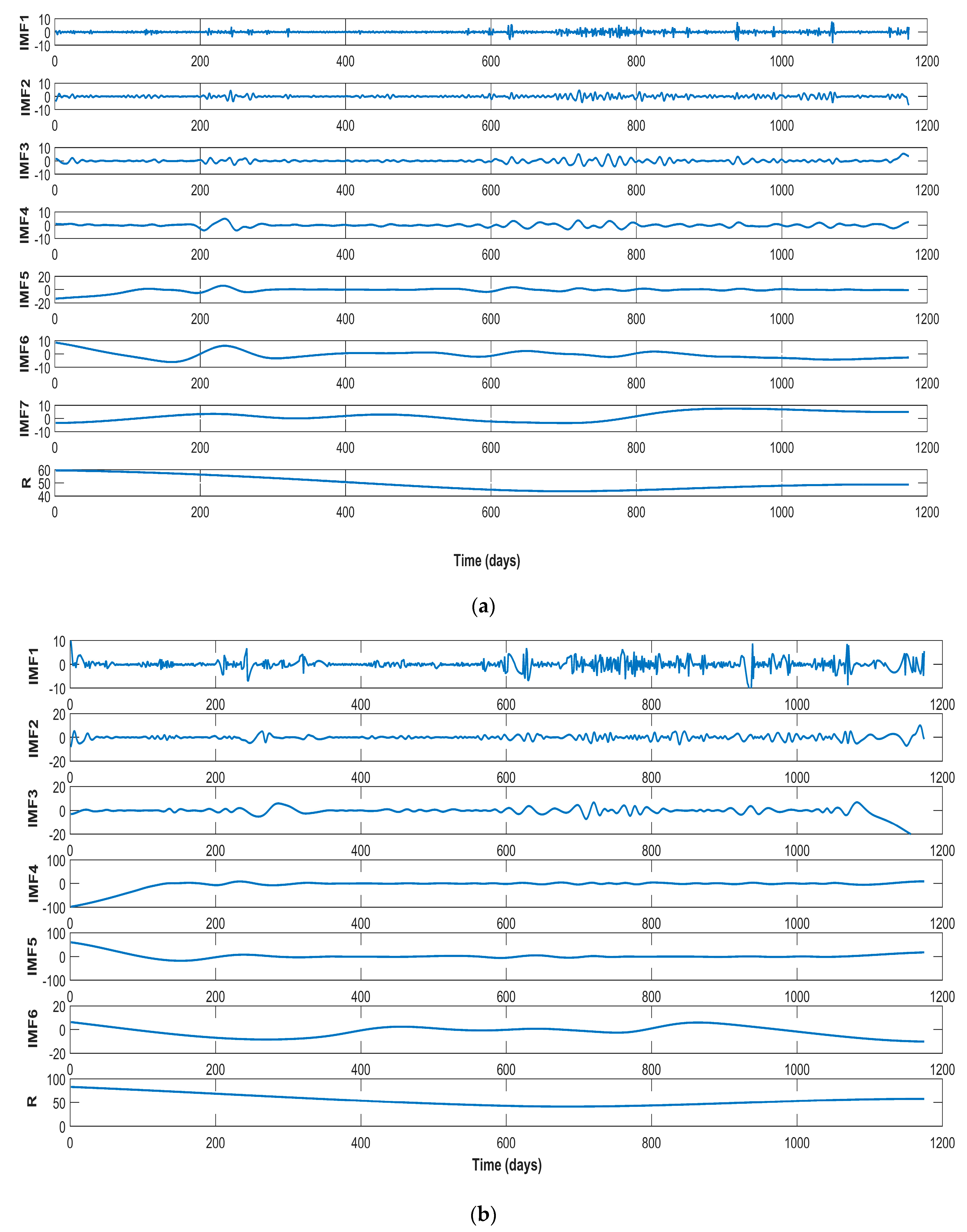
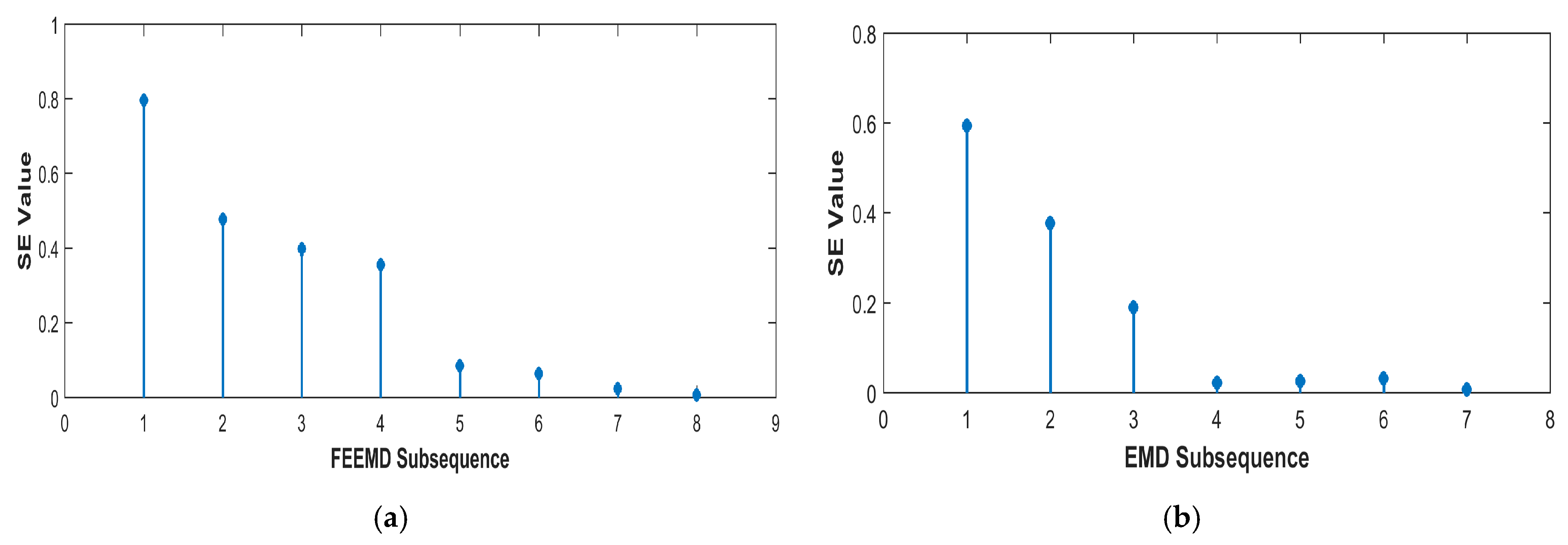
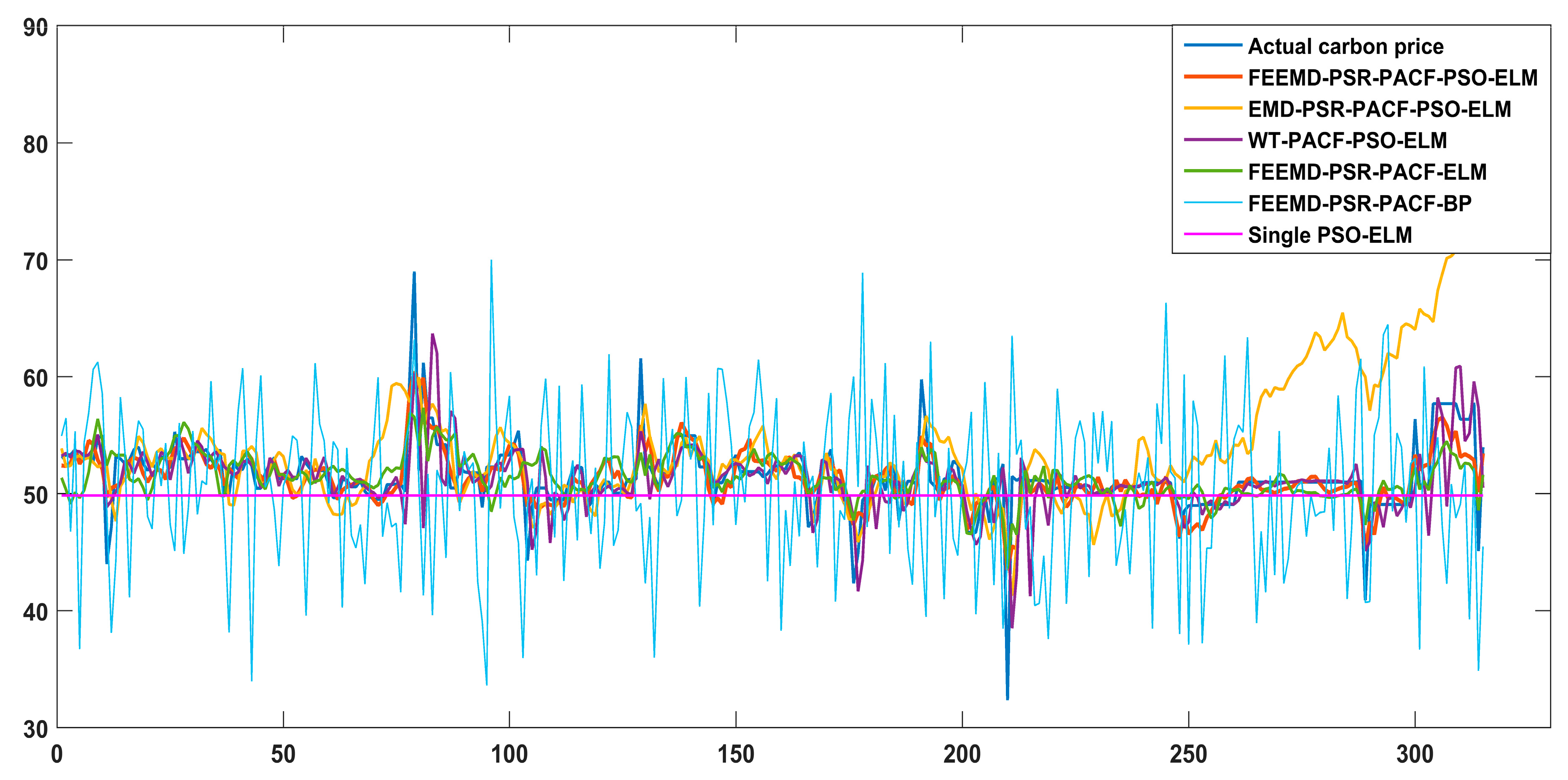
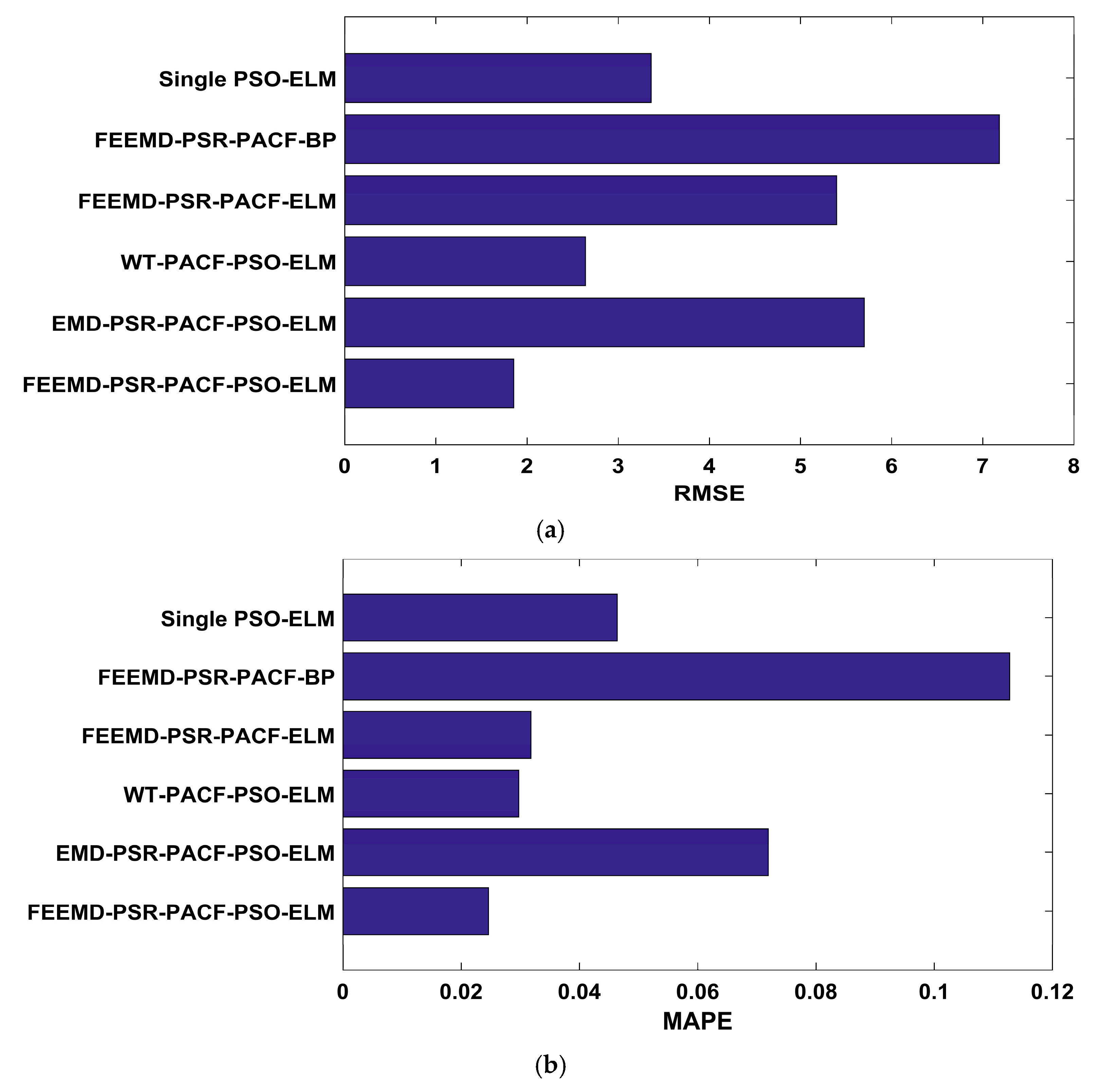
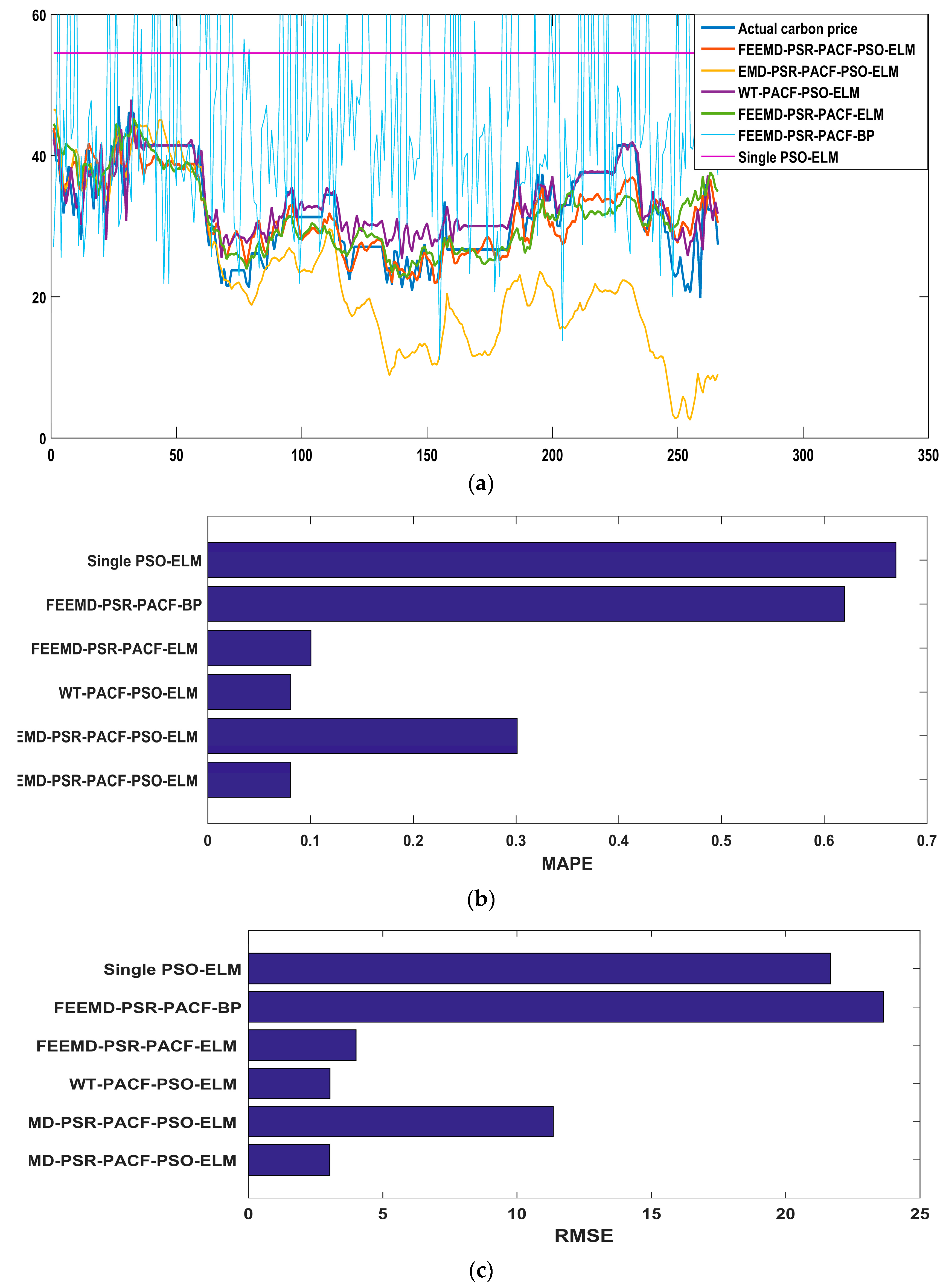
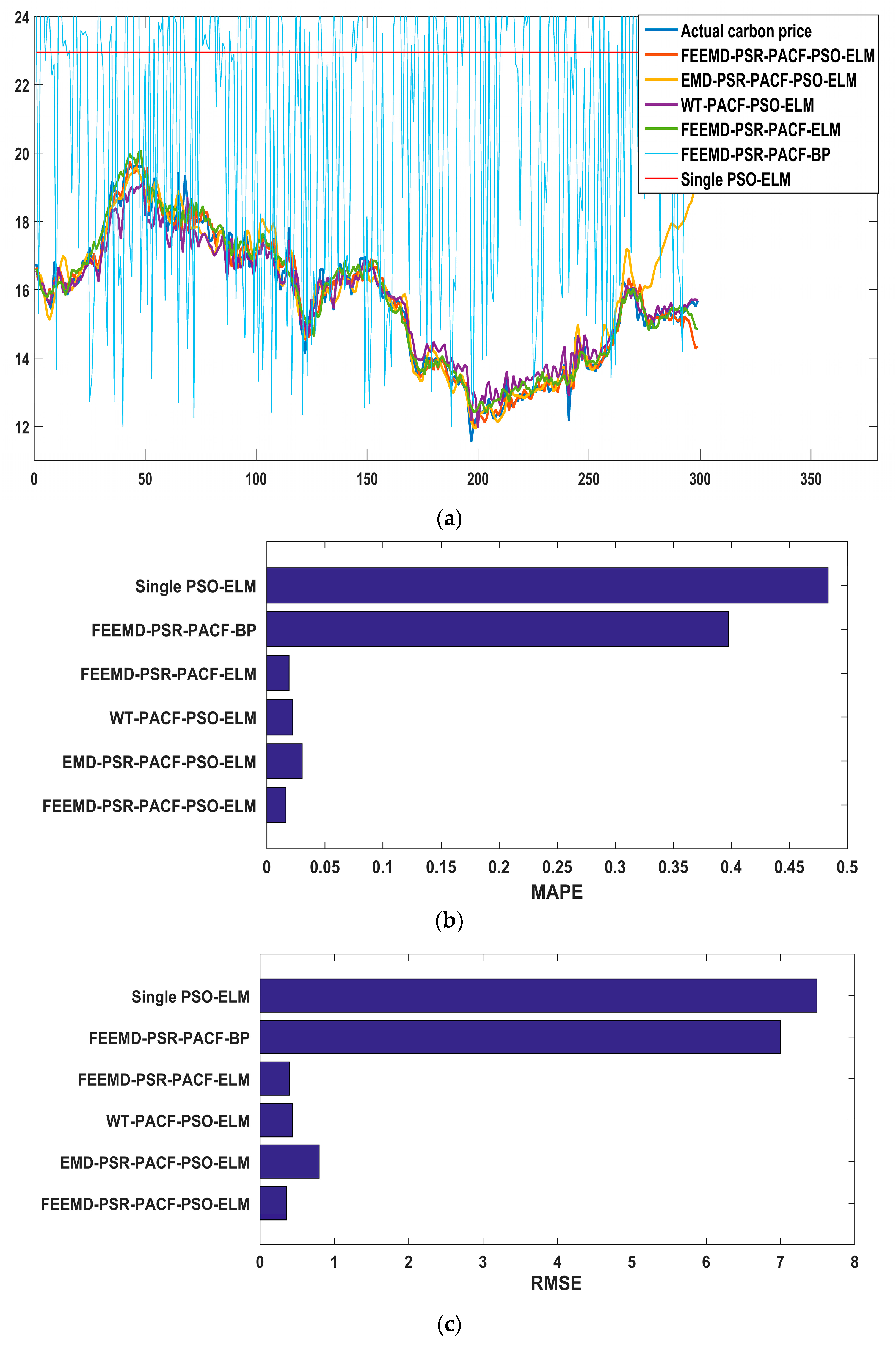
The promotion of the carbon market is a requirement for the high-quality development of China’s economy. An accurate carbon price forecasting method is helpful for the stability of the carbon market. This paper proposed a new hybrid model for carbon price prediction based on fast ensemble empirical mode decomposition, sample entropy, phase space reconstruction, and a partial autocorrelation function that utilizes an extreme learning machine improved by particle swarm optimization. Due to the nonlinearity and volatility of carbon price time series, this paper combined a decomposition method and a phase space reconstruction theory for data analysis and processing. FEEMD was introduced to decompose the original carbon price to reduce the noise signal. The sample entropy was calculated to merge the series decomposed by FEEMD to form new subsequences, which reduced the overall computational workload. Based on Chaos theory, a phase space reconstruction and the maximum Lyapunov exponent were employed to determine the input and output variables of the prediction models. In particular, this paper tested the chaotic property of each subsequence by calculating the maximum Lyapunov exponent, and performed a PACF analysis of the subsequences that were not suitable for PSR. This paper forecast the carbon price using the PSO-ELM model. The decomposition methods and prediction models, including WT, EMD, single ELM, and BP, were compared. To verify the performance and validity of FEEMD-PSR-PACF-PSO-ELM, case studies of three different carbon markets were used. Moreover, we focused on the carbon price forecast under Beijing’s ETS. The conclusions that can be drawn according to the empirical results are summarized below.

(a) Through the performance of the forecasting models in the case studies, we can infer that the decomposition methods (FEEMD, EMD, WT) can improve the forecasting accuracy by reducing the noise interference in the initial data on the carbon price. In the comparison of the decomposition methods, the FEEMD method has better applicability for forecasting the carbon price when applying the same prediction models.

(b) Integrating the Chaos and PACF methods leads to an effective method for processing nonstationary and nonlinear carbon prices that takes full account of the characteristics of the carbon price subsequences.

(c) The PSO-ELM model has the best performance in forecasting the carbon price compared with the other models that were considered in this paper. Taking only historical data into account to determine the input and output of the forecasting models, and following the above-described technical route, we can obtain future carbon price changes in regional carbon markets in China through the proposed model, which contributes to policy development and investment. Moreover, it may be useful for the analysis of the national carbon market.

This paper focuses on the study of historical time series of carbon prices, and fully considers the instability and nonlinear properties of carbon price series. The applicability of the proposed hybrid model was also verified by case studies. However, we did not analyze possible influencing factors in this paper. Therefore, subsequent research may focus on external influencing factors of the carbon price in China’s carbon market.

References

1. Sun, W.; Wang, C.F.; Zhang, C.C. Factor analysis and forecasting of CO2 emissions in Hebei, using extreme learning machine based on particle swarm optimization. J. Clean. Prod. 2017, 162, 1095–1101. [Google Scholar] [CrossRef]
2. Tsai, M.T.; Kuo, Y.T. A Forecasting System of Carbon Price in the Carbon Trading Markets Using Artificial Neural Network. Int. J. Environ. Sci. Dev. 2013, 4, 163–167. [Google Scholar] [CrossRef]
3. Zhu, B.Z.; Shi, X.T.; Chevallier, J.; Wang, P.; Wei, Y.M. An adaptive multiscale ensemble learning paradigm for nonstationary and nonlinear energy price time series forecasting. J. Forecast. 2016, 35, 633–651. [Google Scholar] [CrossRef]
4. Lin, W.B.; Liu, B. Chinese carbon market: Current status and future perspectives. J. Tsinghua Univ. Sci. Technol. 2015, 55, 1315–1323. [Google Scholar]
5. Peng, S.Z.; Chang, Y.; Zhang, J.T. Considerations on Some Key Issues of Carbon Market Development in China. China Popul. Resour. Environ. 2014, 24, 1–5. [Google Scholar] [CrossRef]
6. Huang, Z.P. Does the carbon emission trading scheme promote carbon mitigation. J. Arid Land Resour. Environ. 2018, 32, 32–36. [Google Scholar]
7. Zeng, S.H.; Nan, X.; Liu, C.; Chen, J.Y. The response of the Beijing carbon emissions allowance price (BJC) to macroeconomic and energy price indices. Energy Policy 2017, 106, 111–121. [Google Scholar] [CrossRef]
8. Zhu, B.Z.; Wei, Y.M. Carbon price forecasting with a novel hybrid ARIMA and least squares support vector machines methodology. Omega 2013, 41, 517–524. [Google Scholar] [CrossRef]
9. Xia, R.T. The fluctuant features of China’s carbon emission trading prices. China Price 2018, 5, 52–54. [Google Scholar]
10. Byun, S.J.; Cho, H.J. Forecasting carbon futures volatility using GARCH models with energy volatilities. Energy Econ. 2013, 40, 207–221. [Google Scholar] [CrossRef]
11. Zhang, Y.J.; Yao, T.; He, L.Y.; Ripple, R. Volatility forecasting of crude oil market: Can the regime switching GARCH model beat the single-regime GARCH models? Int. Rev. Econ. Financ. 2018. [Google Scholar] [CrossRef]
12. Basith, S.; Manavalan, B.; Shin, T.H.; Lee, G. iGHBP: Computational identification of growth hormone binding proteins from sequences using extremely randomised tree. Comput. Struct. Biotechnol. J. 2018, 16, 412–420. [Google Scholar] [CrossRef] [PubMed]
13. Wei, L.; Hu, J.; Li, F.Y.; Song, J.N.; Su, R.; Zou, Q. Comparative analysis and prediction of quorum-sensing peptides using feature representation learning and machine learning algorithms. Briefings Bioinform. 2018. [Google Scholar] [CrossRef]
14. Manavalan, B.; Shin, T.H.; Kim, M.O.; Lee, G. PIP-EL: A New Ensemble Learning Method for Improved Proinflammatory Peptide Predictions. Front. Immunol. 2018, 9, 1783. [Google Scholar] [CrossRef]
15. Manavalan, B.; Govindaraj, R.G.; Shin, T.H.; Kim, M.O.; Lee, G. iBCE-EL: A New Ensemble Learning Framework for Improved Linear B-Cell Epitope Prediction. Front. Immunol. 2018, 9, 11. [Google Scholar] [CrossRef]
16. Wei, L.; Chen, H.; Su, R. M6APred-EL: A Sequence-Based Predictor for Identifying N6-methyladenosine Sites Using Ensemble Learning. Mol. Ther. Nucl. Acids 2018, 12, 635–644. [Google Scholar] [CrossRef]
17. Manayalan, B.; Subramaniyam, S.; Shin, T.H.; Kim, M.O.; Lee, G. Machine-Learning-Based Prediction of Cell-Penetrating Peptides and Their Uptake Efficiency with Improved Accuracy. J. Proteome Res. 2018, 17, 2715–2726. [Google Scholar] [CrossRef]
18. Manavalan, B.; Lee, J. SVMQA: Support-vector-machine-based protein single-model quality assessment. Bioinformatics 2017, 33, 2496–2503. [Google Scholar] [CrossRef]
19. Wei, L.; Tang, J.; Zou, Q. SkipCPP-Pred: An improved and promising sequence-based predictor for predicting cell-penetrating peptides. BMC Genom. 2017. [Google Scholar] [CrossRef]
20. Manavalan, B.; Basith, S.; Shin, T.H.; Choi, S.; Kim, M.O.; Lee, G. MLACP: Machine-learning-based prediction of anticancer peptides. Oncotarget 2017, 8, 77121–77136. [Google Scholar] [CrossRef]
21. Dao, F.Y.; Lv, H.; Wang, F.; Feng, C.Q.; Ding, H.; Chen, W.; Lin, H. Identify origin of replication in Saccharomyces cerevisiae using two-step feature selection technique. Bioinformatics 2018. [Google Scholar] [CrossRef]
22. Manavalan, B.; Shin, T.H.; Kim, M.O.; Lee, G. AIPpred: Sequence-Based Prediction of Anti-inflammatory Peptides Using Random Forest. Front. Immunol. 2018, 9, 276. [Google Scholar] [CrossRef] [PubMed]
23. Wei, L.Y.; Zhou, C.; Chen, H.R.; Song, J.N.; Su, R. ACPred-FL: A sequence-based predictor using effective feature representation to improve the prediction of anti-cancer peptides. Bioinformatics 2018, 34, 4007–4016. [Google Scholar] [CrossRef] [PubMed]
24. Manavalan, B.; Shin, T.H.; Lee, G. DHSpred: Support-vector-machine-based human DNase I hypersensitive sites prediction using the optimal features selected by random forest. Oncotarget 2018, 9, 1944–1956. [Google Scholar] [CrossRef] [PubMed]
25. Liu, Z.Y.; Sun, Z.D. The Carbon Trading Price and Trading Volume Forecast in Shanghai City by BP Neural Network. Int. J. Econ. Manag. Eng. 2017, 11, 623–629. [Google Scholar]
26. Zhang, J.L.; Li, D.Z.; Hao, Y.; Tan, Z.F. A hybrid model using signal processing technology, econometric models and neural network for carbon spot price forecasting. J. Clean. Prod. 2018, 204, 958–964. [Google Scholar] [CrossRef]
27. Tsai, M.T.; Kuo, Y.T. Application of Radial Basis Function Neural Network for Carbon Price Forecasting. Appl. Mech. Mater. 2014, 590, 683–687. [Google Scholar] [CrossRef]
28. Gao, Y.; Li, J. International Carbon Finance Market Price Prediction Based on EMD-PSO-SVM Error Correction Model. China Popul. Resour. Environ. 2014, 24, 163–170. [Google Scholar]
29. Razak, I.A.W.A.; Abidin, I.Z.; Yap, K.S.; Abidin, A.A.Z.; Rahman, T.K.A.; Nasir, M.N.M. A novel hybrid method of LSSVM-GA with multiple stage optimization for electricity price forecasting. IEEE Int. Conf. Power Energy 2017, 390–395. [Google Scholar] [CrossRef]
30. Zhu, B.Z.; Ye, S.X.; Wang, P.; He, K.J.; Wei, Y.M. A novel multiscale nonlinear ensemble leaning paradigm for carbon price forecasting. Energy Econ. 2018, 70, 143–157. [Google Scholar] [CrossRef]
31. Huang, G.B.; Zhu, Q.Y.; Siew, C.K. Extreme learning machine: Theory and applications. Neurocomputing 2006, 70, 489–501. [Google Scholar] [CrossRef] [Green Version]
32. Shrivastava, N.A.; Panigrahi, B.K. A hybrid wavelet-ELM based short term price forecasting for electricity markets. Int. J. Electr. Power Energy Syst. 2014, 55, 41–50. [Google Scholar] [CrossRef]
33. Liu, H.; Mi, X.; Li, Y. An Experimental Investigation of Three New Hybrid Wind Speed Forecasting Models Using Multi-decomposing Strategy and ELM Algorithm. Renew. Energy 2018, 123, 694–705. [Google Scholar] [CrossRef]
34. Rocha, H.R.O.; Silvestre, L.J.; Celeste, W.C.; Coura, D.J.C.; Junior, L.O.R. Forecast of Distributed Electrical Generation System Capacity Based on Seasonal Micro Generators using ELM and PSO. IEEE Latin Am. Trans. 2018, 16, 1136–1141. [Google Scholar] [CrossRef]
35. Fan, W.; Tian, L.; Wang, C.; Feng, Z.M.; Wu, D.L.; Li, C.F. Short-term power load forecasting based on PSO-ELM model. J. Nanyang Inst. Technol. 2017, 9, 12–15. [Google Scholar]
36. Saber, T.; Miadreza, S.K.; Gerardo, J.O.; Wang, F.; Alireza, H.; Catalão, J.P.S. Price Forecasting of Electricity Markets in the Presence of a High Penetration of Wind Power Generators. Sustainability 2017, 9, 2065. [Google Scholar] [Green Version]
37. Li, W.; Lu, C. The research on setting a unified interval of carbon price benchmark in the national carbon trading market of China. Appl. Energy 2015, 155, 728–739. [Google Scholar] [CrossRef]
38. Zhu, B.Z.; Han, D.; Wang, P.; Wu, Z.C.; Zhang, T.; Wei, Y.M. Forecasting carbon price using empirical mode decomposition and evolutionary least squares support vector regression. Appl. Energy 2017, 191, 521–530. [Google Scholar] [CrossRef]
39. Wu, Z.; Huang, N.E. Ensemble empirical mode decomposition: A noise-assisted data analysis method. Adv. Adapt. Data Anal. 2009, 1, 1–41. [Google Scholar] [CrossRef]
40. Wang, Y.H.; Yeh, C.H.; Young, H.W.V.; Hu, K.; Lo, M.T. On the computational complexity of the empirical mode decomposition algorithm. Phys. A 2014, 400, 159–167. [Google Scholar] [CrossRef]
41. Heng, J.; Wang, C.; Zhao, X.; Xiao, L. Research and Application Based on Adaptive Boosting Strategy and Modified CGFPA Algorithm: A Case Study for Wind Speed Forecasting. Sustainability 2016, 8, 235. [Google Scholar] [CrossRef]
42. Sun, W.; Liu, M.H. Wind speed forecasting using FEEMD echo state networks with RELM in Hebei, China. Energy Convers. Manag. 2016, 114, 197–208. [Google Scholar] [CrossRef]
43. Sun, W.; Liu, M.H.; Liang, Y. Wind Speed Forecasting Based on FEEMD and LSSVM Optimized by the Bat Algorithm. Energies 2015, 8, 6585–6607. [Google Scholar] [CrossRef] [Green Version]
44. Kennedy, J.; Eberhart, R.C. Particle swarm optimization. In Proceedings of the IEEE International Conference on Neutral Networks (ICNN’95), Perth, Australia, 27 November–1 December 1995; pp. 1942–1948. [Google Scholar]
45. Richman, J.S.; Moorman, J.R. Physiological time-series analysis using approximate entropy and sample entropy. Am. J. Physiol. Heart Circul. Physiol. 2000, 278, 2039–2049. [Google Scholar] [CrossRef] [PubMed]
46. Beoing, G. Visual Analysis of Nonlinear Dynamical Systems: Chaos, Fractals, Self-Similarity and the Limits of Prediction. Systems 2016, 4, 37. [Google Scholar] [CrossRef]
47. Wolf, A.; Jack, B.; Swift, H.L.; Swinney, J.A.V. Determining Lyapunov exponents from a time series. Phys. D-Nonlinear Phenom. 1985, 16, 285–317. [Google Scholar] [CrossRef] [Green Version]
Figure 1. The topology of the extreme learning machine (ELM).
Energies 12 00277 g001
Figure 2. The flow chart of the particle swarm optimization (PSO)-ELM model.
Energies 12 00277 g002
Figure 3. The framework of the proposed forecasting models. IMF, intrinsic mode function. PACF, partial autocorrelation function.
Energies 12 00277 g003
Figure 4. The carbon price graph of the three regional carbon markets.
Energies 12 00277 g004
Figure 5. (a) The fast ensemble empirical mode decomposition (FEEMD) outcome of the Beijing carbon price series; (b) The outcome by the empirical mode decomposition (EMD) method.
Energies 12 00277 g005
Figure 6. The wavelet transform (WT) results on the Beijing carbon price series.
Energies 12 00277 g006
Figure 7. (a) The SE value of subsequences processed by FEEMD; (b) The SE value of subsequences processed by EMD.
Energies 12 00277 g007
Figure 8. (a) The result of the partial autocorrelation function (PACF) analysis of sub4 after processing by FEEMD of the Beijing carbon price; (b) The result of the PACF analysis of sub5 after processing by FEEMD of the Beijing carbon price.
Energies 12 00277 g008
Figure 9. (a) The result of the PACF analysis of sub4 after processing by EMD of the Beijing carbon price; (b) The result of the PACF analysis of A1 after processing by WT of the Beijing carbon price.
Energies 12 00277 g009
Figure 10. The framework of the forecasting models under comparison. BPNN, back propagation neural network.
Energies 12 00277 g010
Figure 11. The forecasting curves of the Beijing carbon price.
Energies 12 00277 g011
Figure 12. The results of the analysis of the carbon price prediction for Beijing. (a) is the root mean square error (RMSE) value; (b) is the mean absolute percentage error (MAPE) value.
Energies 12 00277 g012
Figure 13. (a) The forecasting curves of the Shenzhen carbon price; (b) The MAPE values; (c) The RMSE values.
Energies 12 00277 g013
Figure 14. (a) The carbon price forecasting curves of Hubei; (b) The MAPE values; (c) The RMSE values.
Energies 12 00277 g014
Figure 15. (a) The carbon price forecasting curves; (b) The comparison between the proposed model and the actual carbon price.
Energies 12 00277 g015