Maximum Sensitivity-Constrained Data-Driven Active Disturbance Rejection Control with Application to Airflow Control in Power Plant

 ,
,
Abstract
:1. Introduction
2. Problem Statement
2.1. Processes Model
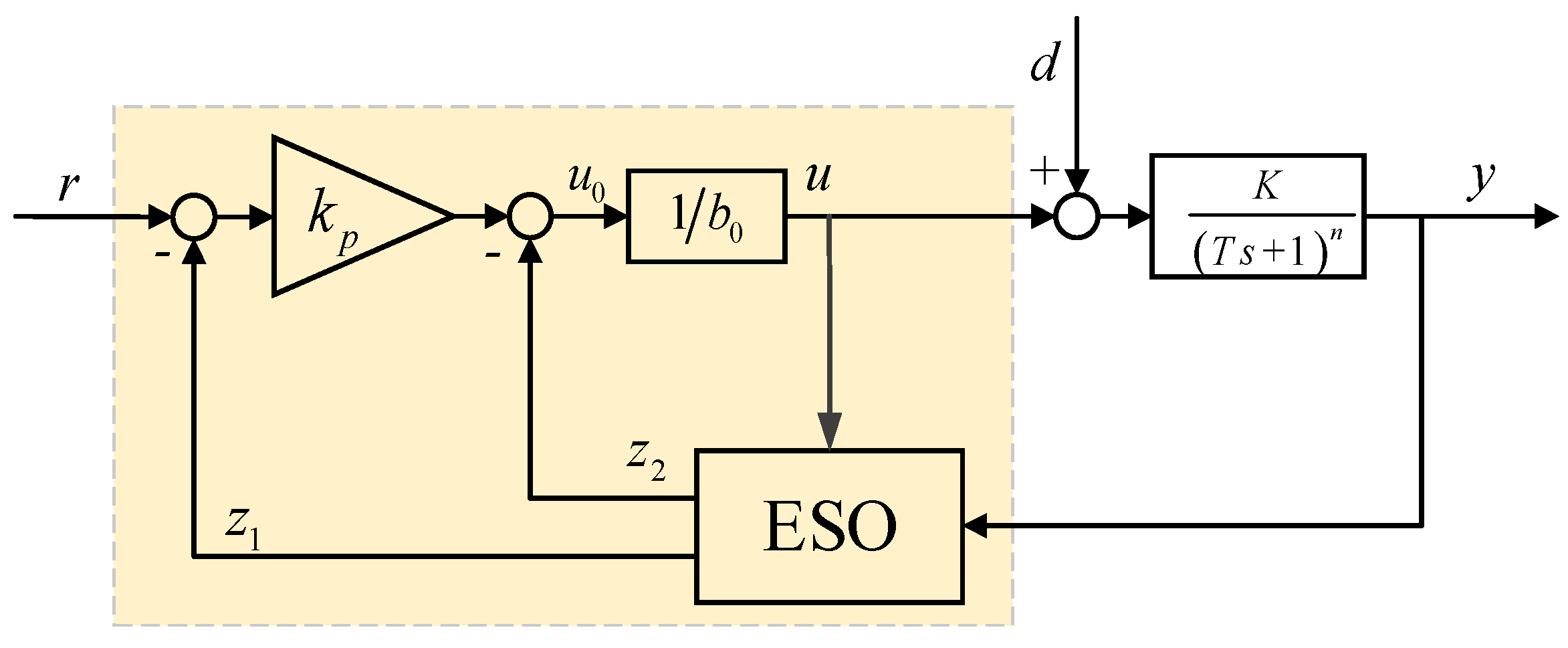
2.2. First-Order Active Disturbance Rejection Control System
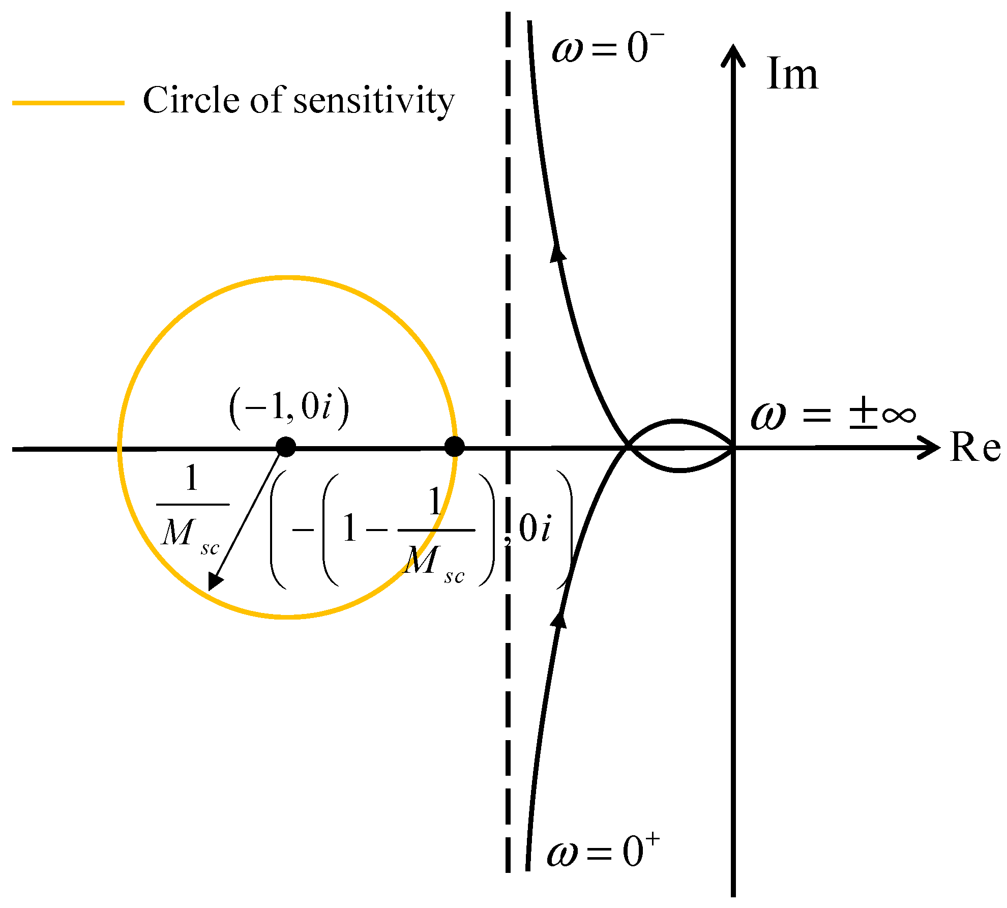
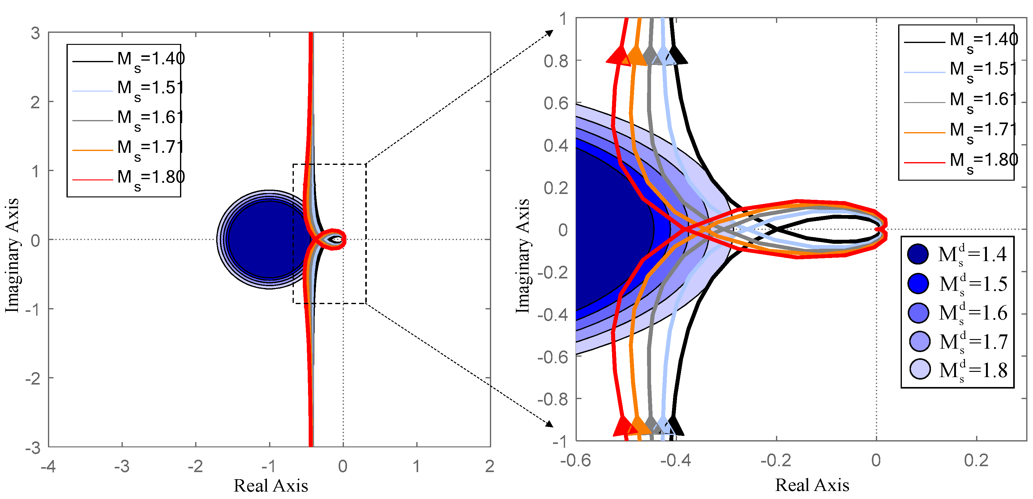
2.3. Maximum Sensitivity
3. Derivation of Parameter Tuning Formulas
3.1. One-Parameter-Tuning Method
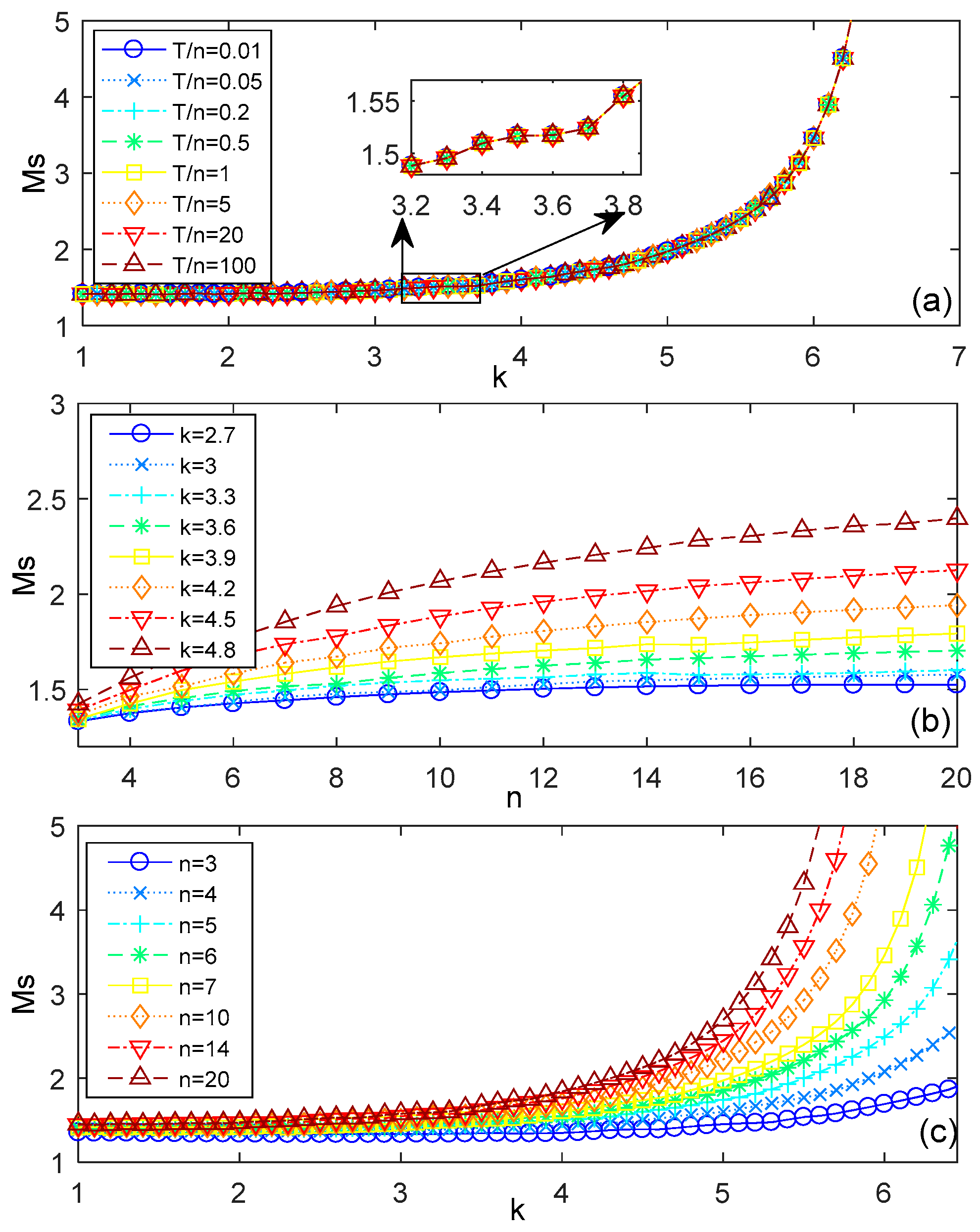
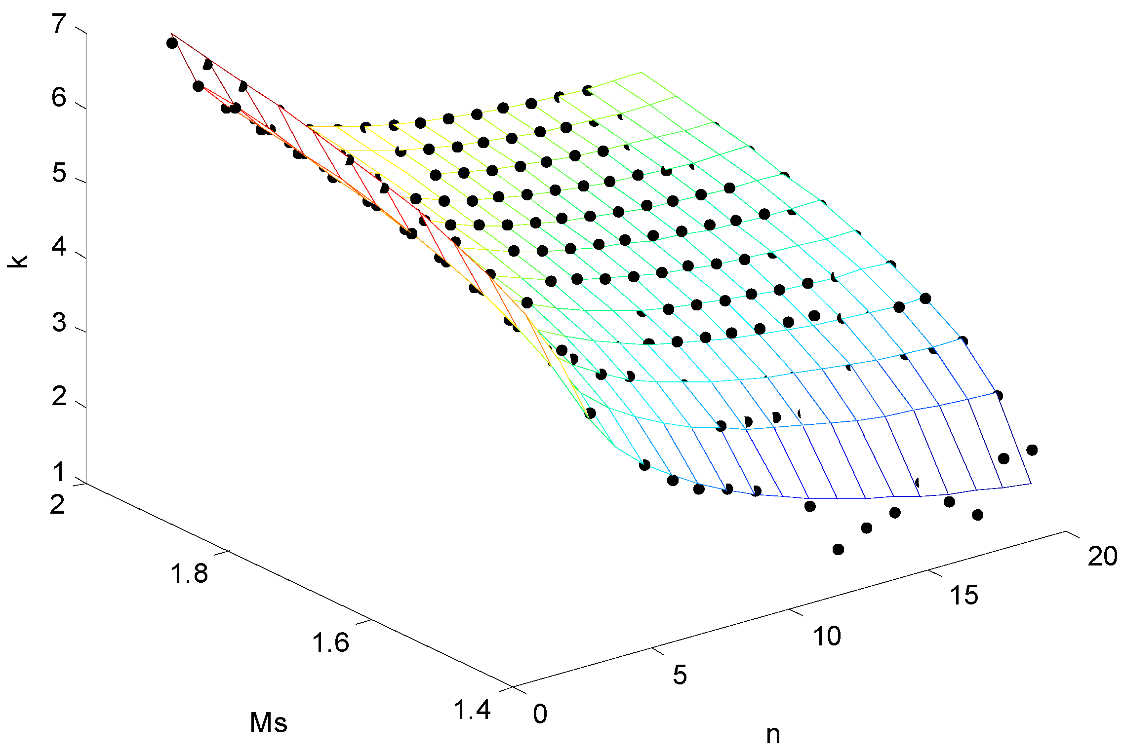
3.2. Relationship between Maximum Sensitivity and Tuning Parameter
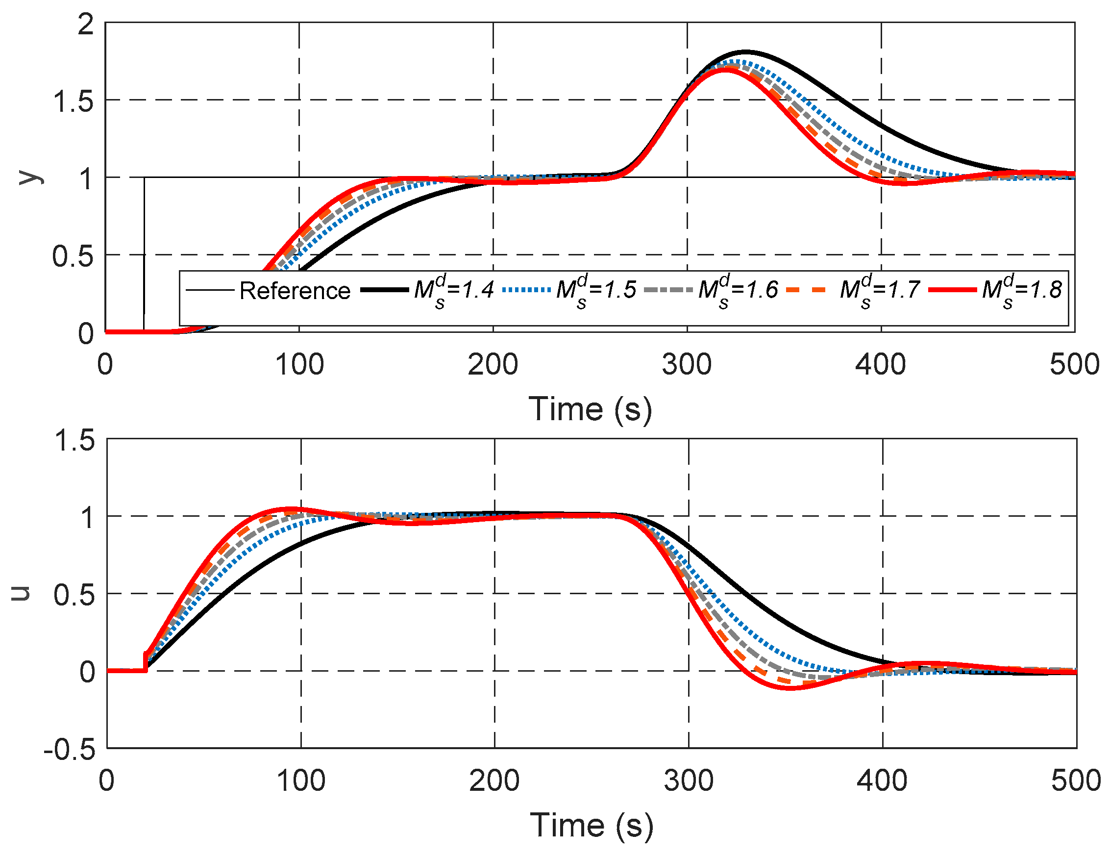
3.3. Illustrative Example
4. Experimental Validation on Power Plant Simulator
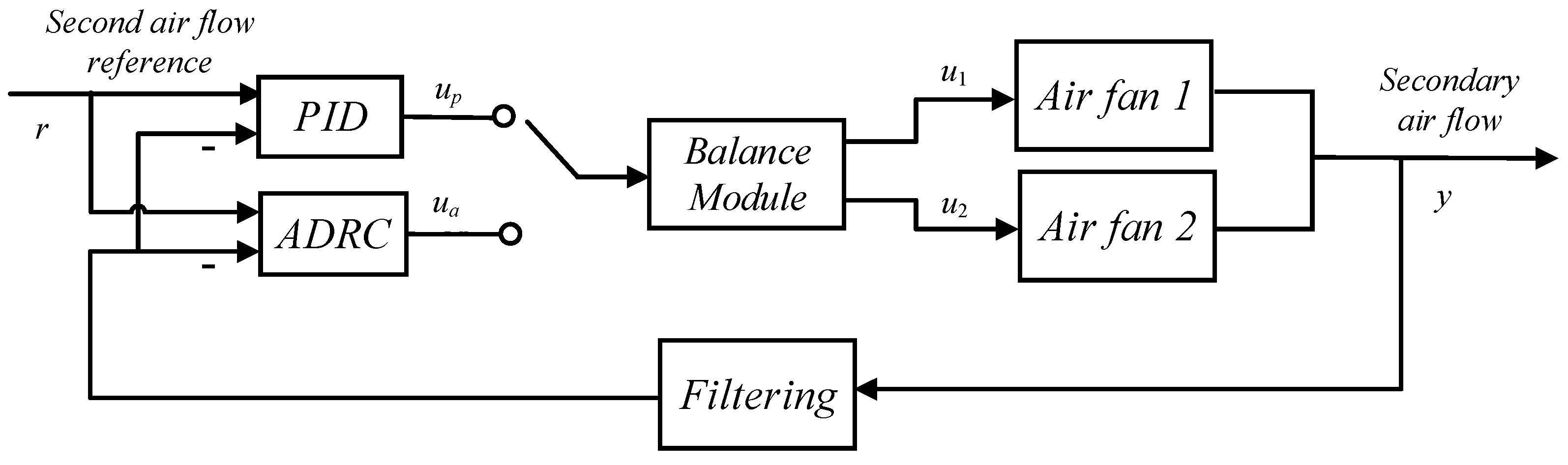
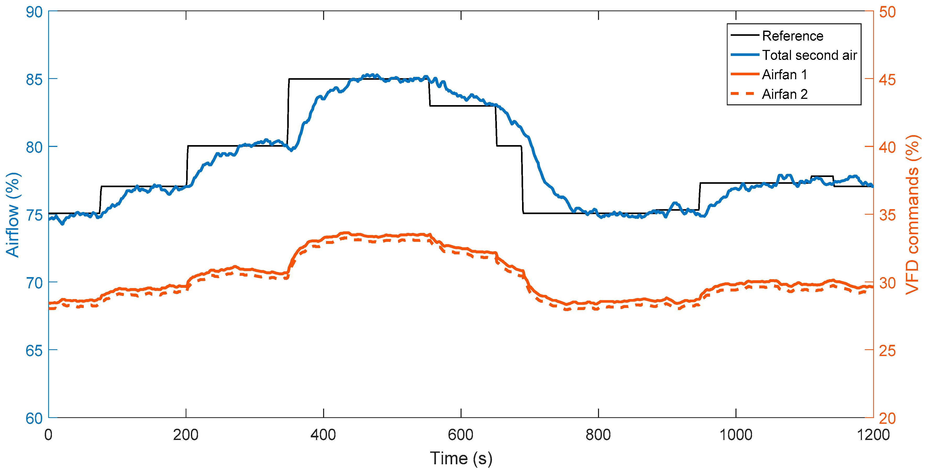
5. Field Test on Secondary Air Control in Actual Power Plant
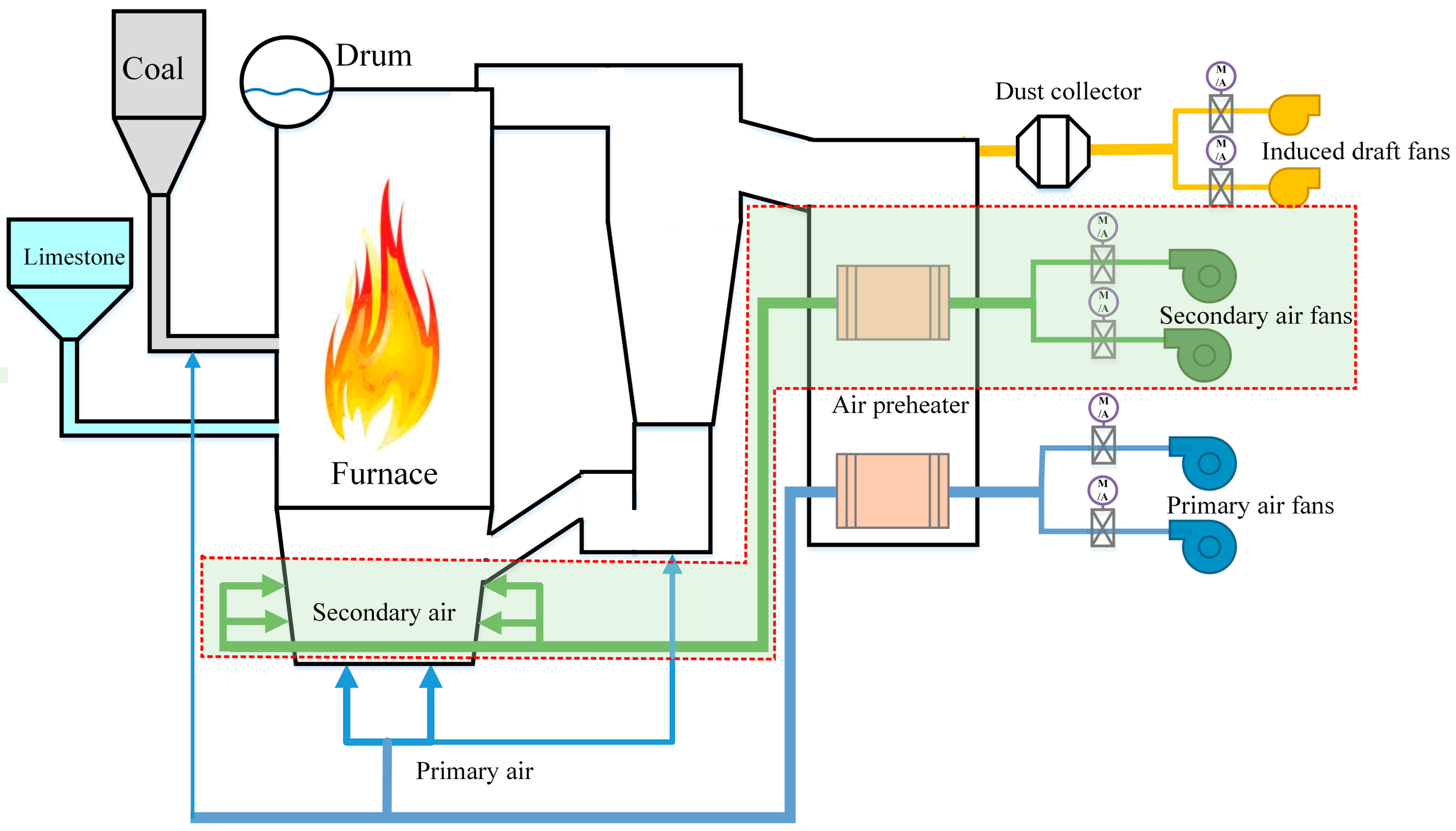
5.1. Process Description
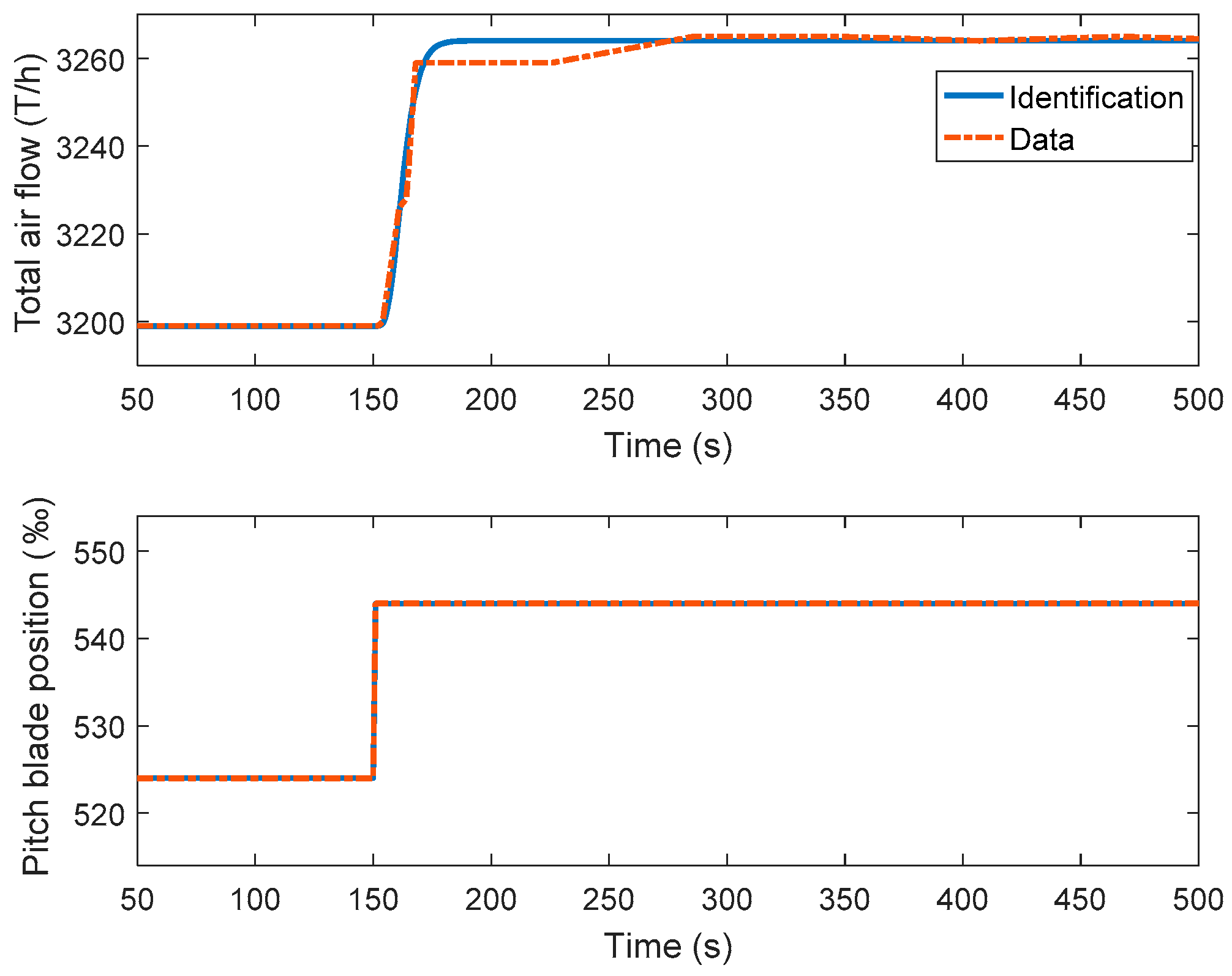
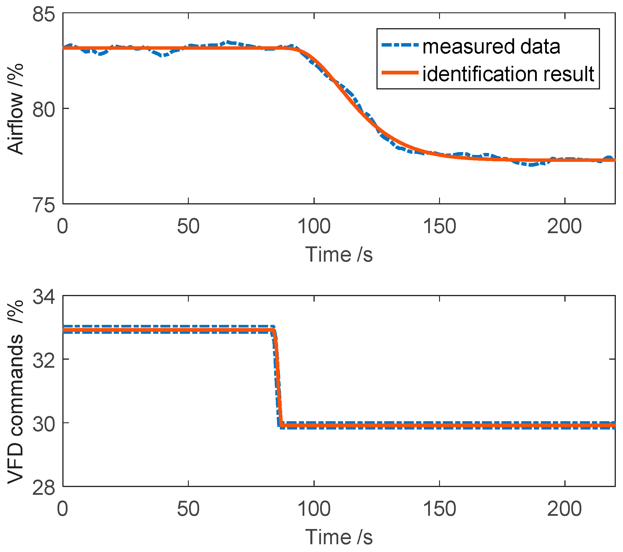
5.2. Process Identification
5.3. Process Identification
6. Conclusions
Author Contributions
Funding
Acknowledgments
Conflicts of Interest
References
- Hiroaki, K. Biological robustness. Nat. Rev. Genet. 2004, 5, 826–837. [Google Scholar]
- Xun, L.; Halbert, W. Robustness checks and robustness tests in applied economics. J. Econ. 2014, 178, 194–206. [Google Scholar]
- Femandez, J.C.; Mounier, L.; Pachon, C. A model-based approach for robustness testing. In Proceedings of the IFIP International Conference on Testing of Communicating System, Montreal, Canada, 31 May–2 June 2005; Springer: Berlin/Heidelberg, Germany; pp. 333–348. [Google Scholar]
- Zames, G. Feedback and optimal sensitivity: Model reference transformations, multiplicative seminorms, and approximate inverses. IEEE Trans. Autom. Control 1981, 26, 301–320. [Google Scholar] [CrossRef]
- Doyle, J. Analysis of feedback systems with structured uncertainties. IEE Proc. D-Control Theor. Appl. 1998, 192, 242–250. [Google Scholar] [CrossRef]
- Braatz, R.; Young, P.; Doyle, J.; Morari, M. Computational complexity of µ calculation. IEEE Trans. Autom. Control 1994, 39, 1000–1002. [Google Scholar] [CrossRef]
- Lesprier, J.; Roos, C.; Biannic, J.; Morari, M. Improved µ upper bound computation using the µ-sensitivities. IFAC-PaperOnLine 2015, 48, 215–220. [Google Scholar] [CrossRef]
- Laura, R.R.; Robert, F.S. A monte carlo approach to the analysis of control system robustness. Automatica 1993, 29, 229–236. [Google Scholar]
- Zhang, Y.; Li, D.; Gao, Z.; Zheng, Q. On oscillation reduction in feedback control for processes with uncertain dead time and internal-external disturbances. ISA Trans. 2015, 59, 29–38. [Google Scholar] [CrossRef]
- He, T.; Li, D.; Wu, Z.; Xue, Y.; Yang, Y. A modified luenberger observer for SOC estimation of lithium-ion battery. In Proceeding of the 36th Chinese Control Conference, Dalian, China, 26–29 July 2017; pp. 924–928. [Google Scholar]
- Persson, P.; Astrom, K.J. Dominant pole design—A unified view of PID controller tuning. Processing of the 4th IFAC Symposium on Adaptive System in Control and Signal, Grenoble, France, 1–3 July 1992; pp. 127–132. [Google Scholar]
- Astrom, K.J.; Hagglund, T. Advanced PID Control; ISA Press Research Triangle Park: Durham, NC, USA, 2006; pp. 111–117. [Google Scholar]
- Astrom, K.J.; Hagglund, T. Design of PI controllers based on non-convex optimization. Automatica 1998, 34, 565–601. [Google Scholar] [CrossRef]
- Yaniv, O.; Nagurka, M. Design of PID controllers satisfying gain margin and sensitivity constraints on a set of plants. Automatica 2004, 40, 111–116. [Google Scholar] [CrossRef]
- Alfaro, V.; Vilanova, R. Model-reference robust tuning of 2DoF PI controllers for first- and second-order plus dead-time controlled processes. J. Process Control 2012, 22, 359–374. [Google Scholar] [CrossRef]
- Li, D.; Liu, L.; Jin, Q.; Hirasawa, K. Maximum sensitivity based fractional IMC-PID controller design for non-integer order system with time delay. J. Process Control 2015, 31, 17–29. [Google Scholar] [CrossRef]
- Han, J. From PID to active disturbance rejection control. IEEE Trans. Ind. Electron 2009, 56, 900–906. [Google Scholar] [CrossRef]
- Gao, Z. Active disturbance rejection control: From an enduring idea to an emerging technology. In Proceedings of the 2015 10th International Workshop on Robot Motion and Control, Poznan, Poland, 6–8 July 2015; pp. 269–282. [Google Scholar]
- Xue, W.; Huang, Y. Performance analysis of active disturbance rejection tracking control for a class of uncertain LTI systems. ISA Trans. 2015, 58, 133–154. [Google Scholar] [CrossRef] [PubMed]
- Hou, Z.; Gao, H.; Lewis, F.L. Data-Driven control and learning systems. IEEE Trans. Ind. Electron. 2017, 64, 4070–4075. [Google Scholar] [CrossRef]
- Han, J.; Wang, H.; Jiao, G.; Cui, L.; Wang, Y. Research on active disturbance rejection control technology of electromechanical actuators. Electronics 2018, 7, 174. [Google Scholar] [CrossRef]
- Roman, R.C.; Radac, M.B.; Tureac, C.; Precup, R.E. Data-Driven active disturbance rejection control of pendulum cart systems. In Proceedings of the Conference on Control Technology and Applications, Copenhagen, Denmark, 21–24 August 2018; pp. 933–938. [Google Scholar]
- Wang, G.; Xu, Q. Sliding mode control with disturbance rejection for piezoelectric nanopositioning control. In Proceedings of the Annual American Control Conference, Milwaukee, WI, USA, 27–29 June 2018; pp. 6144–6149. [Google Scholar]
- Sun, L.; Shen, J.; Hua, Q.; Lee, K.Y. Data-driven oxygen excess ratio control for proton exchange membrane fuel cell. Appl. Energy 2018, 231, 866–875. [Google Scholar] [CrossRef]
- Madoski, R.; Kordasz, M.; Sauer, P. Application of a disturbance-rejection controller for robotic-enhanced limb rehabilitation trainings. ISA Trans. 2014, 53, 899–908. [Google Scholar] [CrossRef]
- Ramirez, N.; Sira, R.; Garrido, M.; Luviano, J. Linear active disturbance rejection control of underactuated systems: The case of the furuta pendulum. ISA Trans. 2014, 53, 920–928. [Google Scholar] [CrossRef]
- Xue, W.; Bai, W.; Yang, S.; Song, K.; Huang, Y.; Xie, H. ADRC with adaptive extended state observer and its application to air-fuel ratio control in gasoline engines. IEEE Trans. Ind. Electron. 2015, 62, 5847–5857. [Google Scholar] [CrossRef]
- Fu, C.; Tan, W. Decentralized load frequency control for power systems with communication delays via active disturbance rejection. IET Gener. Trans. Distrib. 2018, 12, 1397–1403. [Google Scholar]
- Li, S.; Xia, C.; Zhou, X. Disturbance rejection control method for permanent magnet synchronous motor speed-regulation system. Mechatronics 2012, 22, 706–714. [Google Scholar] [CrossRef]
- Li, S.; Li, J. Output predictor-based active disturbance rejection control for a wind energy conversion system with PMSG. IEEE Access 2017, 5, 5205–5214. [Google Scholar] [CrossRef]
- Sun, L.; Li, D.; Hu, K.; Lee, K.Y.; Pan, F. On tuning and practical implementation of ADRC: A case study from a regenerative heater in a 1000 MW power plant. Ind. Eng. Chem. Res. 2016, 55, 6686–6695. [Google Scholar] [CrossRef]
- Gernot, H. Practical active disturbance rejection control: Bumpless transfer, rate limitation and incremental algorithm. IEEE Trans. Ind. Electron. 2016, 63, 1754–1762. [Google Scholar]
- Liu, Z.H.; Zhang, Y.J.; Zhang, J.; Wu, J.H. Active disturbance rejection control of a chaotic system based on immune binary-state particle swarm optimization algorithm. Acta Physica Sinica 2011, 60, 1–9. [Google Scholar]
- Wu, L.; Bao, H.; Du, J.; Wang, C. A learning algorithm for parameters of automatic disturbances rejection controller. Acta Automatica Sinica 2014, 40, 556–560. [Google Scholar]
- Sun, L.; Hua, Q.; Shen, J.; Xue, Y.; Li, D.; Lee, K.Y. Multi-objective optimization for advanced superheater steam temperature control in a 300 MW power plant. Appl. Energy 2017, 208, 592–606. [Google Scholar] [CrossRef]
- Gao, Z. Scaling and bandwidth-parameterization based controller tuning. In Proceedings of the American Control Conference, Denver, CO, USA, 4–6 June 2003; pp. 4989–4996. [Google Scholar]
- Chen, X.; Li, D.; Gao, Z. Tuning method for second-order active disturbance rejection control. In Proceeding of the 30th Chinese Control Conference, Yantai, China, 22–24 July 2011; pp. 6322–6327. [Google Scholar]
- Tan, W.; Fu, C. Linear active disturbance-rejection control: Analysis and tuning via IMC. IEEE Trans. Ind. Electron. 2016, 63, 2350–2359. [Google Scholar] [CrossRef]
- Saptarshi, D.; Suman, S.; Shantanu, D.; Amitava, G. On the selection of tuning methodology of FOPID controllers for the control of higher order processes. ISA Trans. 2011, 50, 376–388. [Google Scholar] [Green Version]
- Malwatkar, G.M.; Sonawana, S.H.; Waghmare, L.M. Tuning PID controllers for high-order oscillatory systems with improved performance. ISA Trans. 2009, 48, 347–353. [Google Scholar] [CrossRef] [PubMed]
- Shao, S.; Gao, Z. On the conditions of exponential stability in active disturbance rejection control based on singular perturbation analysis. Int. J. Control 2017, 90, 2085–2097. [Google Scholar] [CrossRef]
- Kokotovic, P.V.; Khalil, H.K.; O’Reilly, J. Singular Perturbation Methods in Control: Analysis and Design; Society for Industrial and Applied Mathematics: London, UK, 1986. [Google Scholar]
- Zhao, C.; Li, D. Control design for the SISO system with the unknown order and the unknown relative degree. ISA Trans. 2014, 53, 858–872. [Google Scholar] [CrossRef] [PubMed]


| Design Parameter | Controller Parameters | Ms | Tracking | Disturbance Rejection | IAE | TV | ||
|---|---|---|---|---|---|---|---|---|
| Ts/s | σ/% | Ts/s | σ/% | |||||
| = 1.4 | ωc = 0.0790, ωo = 0.7903, b0 = 2.4574 | 1.40 | 189 | 0.73 | 300 | 75.4 | 181.7 | 2.02 |
| = 1.5 | ωc = 0.0503, ωo = 0.5034, b0 = 0.7629 | 1.51 | 155 | 0.26 | 182 | 74.6 | 146.8 | 2.00 |
| = 1.6 | ωc = 0.0440, ωo = 0.4405, b0 = 0.5137 | 1.61 | 138 | 0.74 | 159 | 71.5 | 134.6 | 2.10 |
| = 1.7 | ωc = 0.0408, ωo = 0.4081, b0 = 0.4027 | 1.71 | 127 | 1.25 | 191 | 68.7 | 127.6 | 2.25 |
| = 1.8 | ωc = 0.0387, ωo = 0.3873, b0 = 0.3372 | 1.80 | 200 | 1.53 | 188 | 66.5 | 122.9 | 2.43 |
| Method | Controller Parameters | Ms | Tracking | Disturbance Rejection | IAE | TV | ||
|---|---|---|---|---|---|---|---|---|
| Ts/s | σ/% | Ts/s | σ/% | |||||
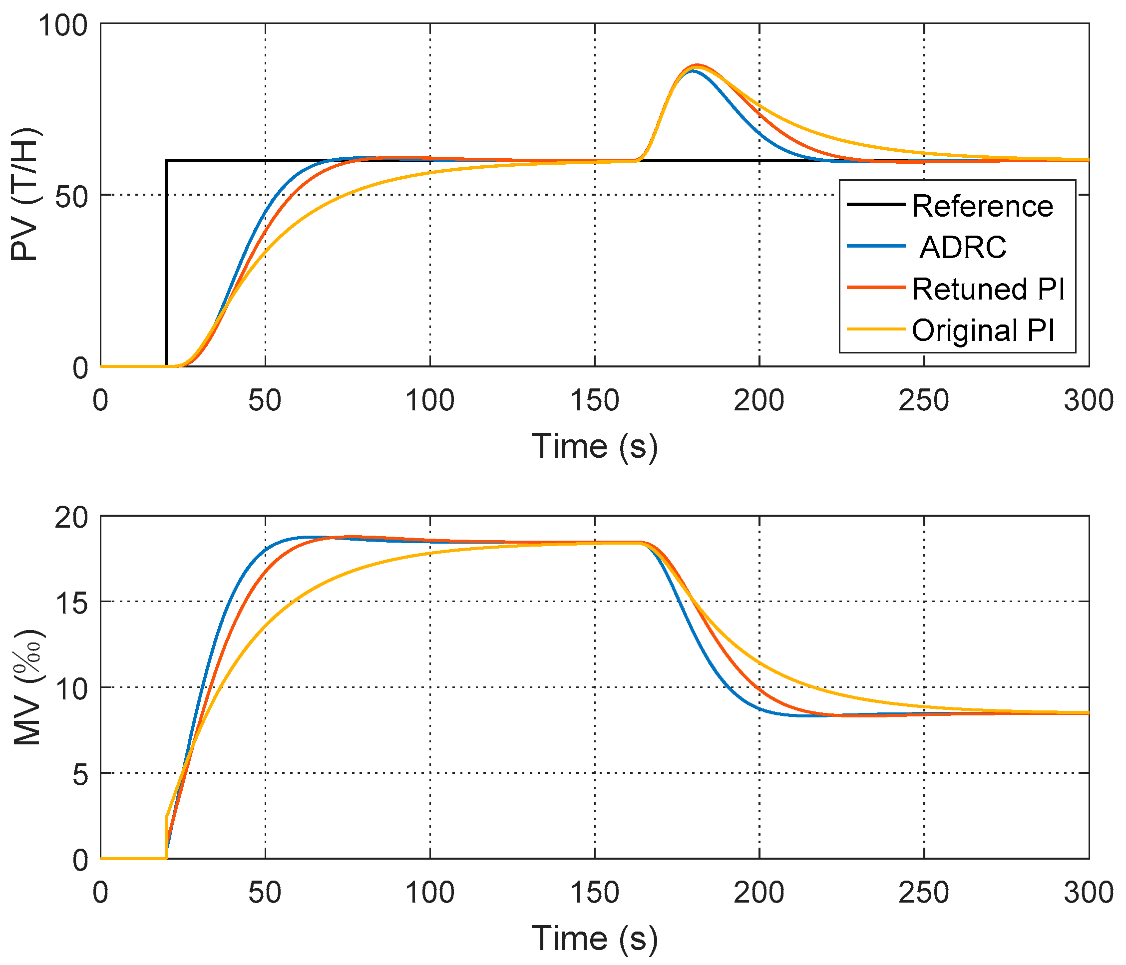
| ADRC | ωc = 0.32, ωo = 3.24, b0 = 32.83 | 1.4 | 45 | 1.2 | 53 | 43.4 | 2097 | 29 |
| Retuned PI | Kp = 0.014, Ki = 0.012 | 1.4 | 53 | 1.2 | 64 | 46.3 | 2450 | 28 |
| Original PI | Kp = 0.04, Ki = 0.009 | 1.1 | 105 | 1.5 | 103 | 45.4 | 3277 | 28 |
| Control Algorithm | Constant Load | Varying Load | |
|---|---|---|---|
| Overshoot σ (%) | (T/h) | ||
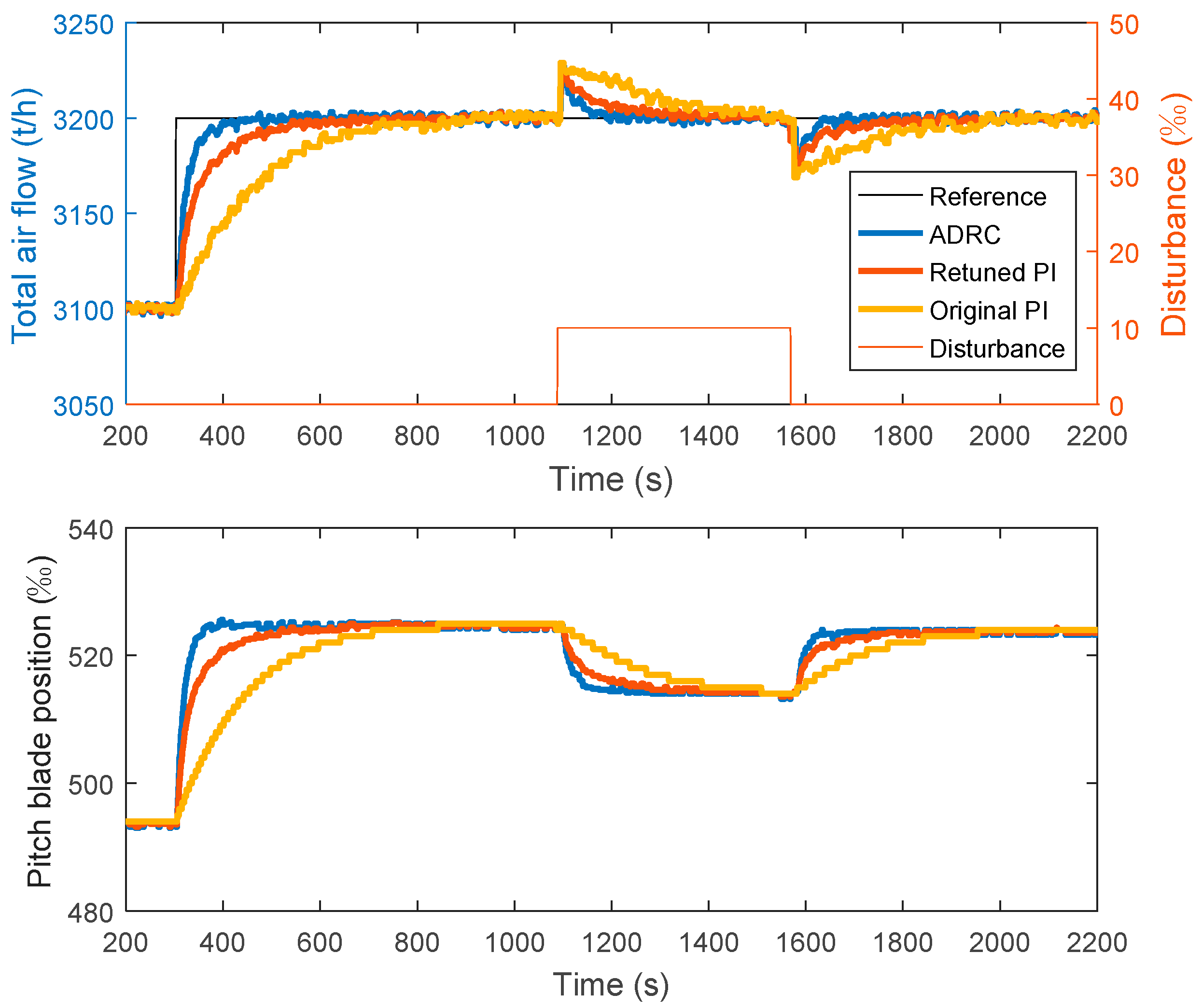
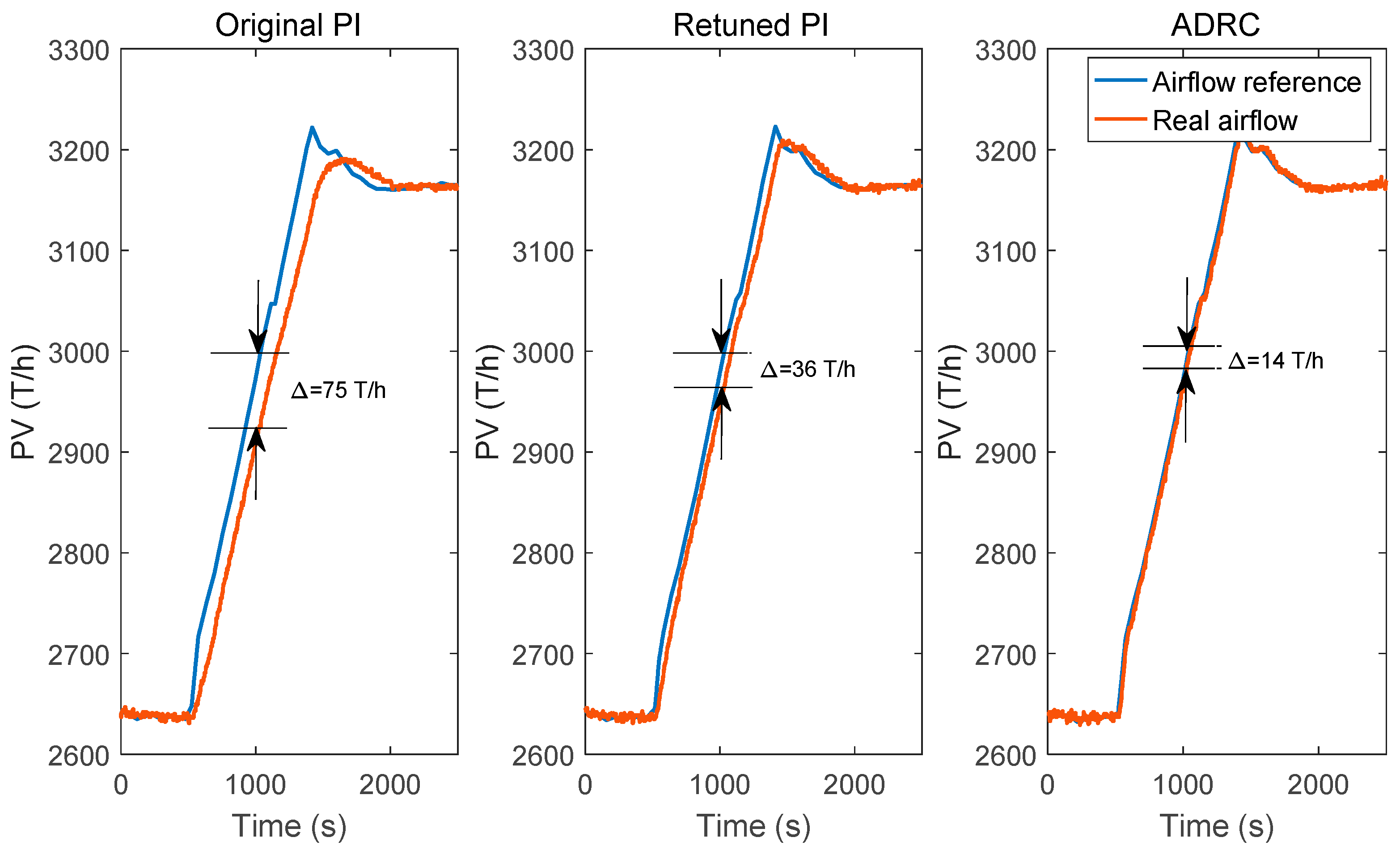
| ADRC | 52.5 | 26.5 | 15.1 |
| Retuned PI | 108 | 28.1 | 31.2 |
| Original PI | 226 | 30.0 | 70.5 |
| Control Algorithm | IAE | ITAE | ||
|---|---|---|---|---|
| ADRC | 86 s | 959 | 5384 | 22.95 |
| PID | >193 s 1 | 1644 | 9041 | 28.17 |
| Improvement | >55.4% | 41.6% | 40.4% | 18.5% |
© 2019 by the authors. Licensee MDPI, Basel, Switzerland. This article is an open access article distributed under the terms and conditions of the Creative Commons Attribution (CC BY) license (http://creativecommons.org/licenses/by/4.0/).
Share and Cite
He, T.; Wu, Z.; Shi, R.; Li, D.; Sun, L.; Wang, L.; Zheng, S. Maximum Sensitivity-Constrained Data-Driven Active Disturbance Rejection Control with Application to Airflow Control in Power Plant. Energies 2019, 12, 231. https://doi.org/10.3390/en12020231
He T, Wu Z, Shi R, Li D, Sun L, Wang L, Zheng S. Maximum Sensitivity-Constrained Data-Driven Active Disturbance Rejection Control with Application to Airflow Control in Power Plant. Energies. 2019; 12(2):231. https://doi.org/10.3390/en12020231
Chicago/Turabian StyleHe, Ting, Zhenlong Wu, Rongqi Shi, Donghai Li, Li Sun, Lingmei Wang, and Song Zheng. 2019. "Maximum Sensitivity-Constrained Data-Driven Active Disturbance Rejection Control with Application to Airflow Control in Power Plant" Energies 12, no. 2: 231. https://doi.org/10.3390/en12020231