Traveling Waves-Based Method for Fault Estimation in HVDC Transmission System


Department of Electrical Engineering, University of Lahore, Lahore 54000, Pakistan
Energies 2019, 12(19), 3614; https://doi.org/10.3390/en12193614
Submission received: 28 August 2019
/
Revised: 15 September 2019
/
Accepted: 18 September 2019
/
Published: 21 September 2019
Abstract
:The HVDC transmission system is winning hearts of researchers and electrical engineers because of its notable merits as compared to the HVAC transmission system in the case of long-distance bulk power transmission. The HVDC transmission system is known for its low losses, effective control ability, efficiency and reliability. However, because of the sudden build-up of fault current in the HVDC transmission system, conventional relays and circuit breakers are required to be modified. Detection of fault location is an important parameter of protection of the HVDC transmission system. In this research paper, fault location methods based on traveling waves are reviewed for the HVDC transmission system. Arrival time and natural frequency are the two parameters of measurement in traveling waves. Advantages and disadvantages of methods of traveling waves with respect to their quantities of measurements are analyzed critically. Further, a two-terminal HVDC test grid is simulated over Matlab/Simulink. Different types of AC and DC faults and at different locations are analyzed on a test grid. A traveling wave-based technique of fault estimation is developed and is evaluated for identification, classification and finding location of faults to validate its performance. Moreover, this technique is supported with analysis of fast Fourier transform to accelerate its practicality and realization.
1. Introduction
With an increasing demand of energy, there is a need to reshape the concept of power generating and transferring. These modifications and additions must be technically adequate and reasonably economical in order to meet high energy rates and growing load densities at far flung areas in an optimum way. Electrical energy is necessary for all aspects of every day’s life. Therefore, reliability and protection of electrical power system are the crucial parameters for the betterment of human society. In the 20th century, AC dominated in the war of currents because of the development of transformers. Therefore, power was used to transfer through high voltage AC transmission lines. However, with the development of mercury arc valves and thyratron, once again investors and energy sector personnel started looking into deployment of transmission lines carrying DC values of current [1,2,3,4].
The HVDC transmission system is a perfect solution for long distance bulk power transfer. This is made possible because of the advancement in power electronics. As a result, a reliable and sophisticated the HVDC transmission system has been developed. Due to its large-scale deployment in an open environment, chances of faults or abnormalities are high. Therefore, it cannot be left as it is. There is a need to develop or design a protection system that should respond in case of abnormalities or faults. As it is a transmission line, its ends are far apart. Faults can occur at any point between the ends of transmission line. In addition to this, it is crucial for patrolling personnel to find the location of a fault over a widespread network of transmission lines in a versatile landscape. Therefore, this challenge results in a great loss of fault recovery time. Selection of a reliable algorithm for fault estimation with the intentions of minimizing the stress of patrolling personnel, reducing fault recovery time and curtailing revenue losses because of power outage is a compelling matter of necessary engineering application. A lot of research is being conducted to find an accurate location of fault so that effects of faults could be limited or minimized [5,6,7,8,9,10,11].
There are basically two main classifications of fault estimation in transmission lines: impedance method and traveling wave method. Due to low inertia characteristics and difficulties in evaluating impedance for multi-terminal (MT) systems, applications of impedance method for fault estimation are limited. On the other hand, traveling wave method requires a shorter data window. Amplitude and polarity of traveling wave are independent of the effects of events of DC faults initiation, which are dissimilar to events of AC faults initiation. This manifestation makes traveling wave method an ideal technique for fault estimation in HVDC systems [12,13,14,15]. Hence, the proposed research on fault estimation in the HVDC system is based on traveling waves.
Accuracy in finding fault location is an important task. Remedial and precautionary maintenance and continuity of power transfer are greatly influenced by an accurate determination of fault location. Because of considerable errors in reactance and impedance methods for finding fault location, other possibilities are explored [16,17,18]. Distributed parameter model is a technique of fault estimation known for its accuracy of estimation and appropriateness for two terminal system but it is highly challenging to extend it for multi terminal HVDC systems [19]. A single terminal method based on parameter identification is also developed but its employment is limited to transmission systems containing large capacitors in parallel [20]. It is very complicated to determine equivalent impedance of HVDC transmission systems by a natural frequency-based method because of varying impedance of fault due to change in fault location. Further, it cannot be extended to multi-terminal systems because of different geometries of meshed network under different locations of fault. Hence, determination of exact equivalent impedance is crucial [21,22]. A wavelet transform (WT) and artificial neural network (ANN)-based method of fault estimation is also devised. This method is associated with the setting up of many parameters for training neural network and delays in learning for accurate estimation [23]. Determination of maxima of wavelet modulus is another approach of DC protection to estimate fault in HVDC transmission systems but accuracy is compromised particularly in the case of fault location [24]. Up to now, there are few methods of fault estimation in HVDC systems available in literature [25,26] that can be extended to multi-terminal systems without a compromise on accuracy and reliability.
This research paper covers the review of traveling wave-based methods of finding location of faults in HVDC transmission lines. Advantages and shortcomings of these methods under different scenarios are discussed. Analytical behaviors of traveling wave-based methods are critically examined and arguments are built on the basis of derived results available in the literature. Moreover, in this research paper, an accurate and a reliable technique of fault estimation is developed for the HVDC transmission system. This technique utilizes the DC component, dominant AC component and THD values of traveling wave for fault estimation. This technique perfectly identifies, classifies and locates the fault in HVDC transmission systems. Although this method is tested initially for two-terminal system, it can be extended to multi terminal systems effectively.
This research paper consists of the following sections: Section 1 covers the introduction and literature review of the HVDC transmission system and fault location methods. Theoretical background of traveling waves and its relationship with power system protection are discussed in Section 2. The traveling waves method based on measurement of arrival time and its limitations is covered in Section 3. Section 4 consists of the traveling waves method based on measurement of natural frequency and its restraints. Details of the test model of a HVDC transmission system to analyze and to validate the performance of the proposed method of fault estimation are given in Section 5. Simulation results under scenarios of fault identification, fault classification and fault location are discussed in Section 6. Conclusions are drawn in Section 7.
2. Traveling Wave Theory
The concept of usage of the traveling wave phenomenon for finding location of fault originated in 1950. It was applied in commercial products and it was found that it addressed all the inabilities of reactance and impedance methods. However, it was not deployed worldwide because of its limited capability of detection of components. Faults, switching operation and lightning are the common causes of origination of traveling waves. Crossley and McLaren were the pioneers of proposing the phenomenon of traveling waves for fault location estimation in power system protection. They proposed that when a fault commenced, traveling waves were generated at the fault point. These traveling waves propagated from the fault point towards the terminals and returned back. The time required for propagation and returning back is an important hypothesis for estimation of the location of fault. However, it is found challenging from the studies [27,28,29,30,31,32,33,34] to estimate exact location of fault in transmission lines on the basis of determination of propagation time of traveling waves because of variation of propagation distance. Difficulties in the measurement of arrival time, detection of first traveling wave for correlation, identification of fault near terminals because of less noticeable variation in traveling wave make these methods [27,28,29,30,31,32,33] less applicable to real world systems. Further, problems of a probabilistic approach and existence of biasedness in data samples reduce the realization of method of traveling wave [34]. Moreover, these techniques are mature for the high voltage alternating current (HVAC) transmission system where polarity of alternating current (AC) is varied in each cycle but are not favorable for the HVDC transmission system because of different characteristics of DC faults. Therefore, in this proposed research, magnitude of DC component, dominant AC component and THD values of traveling wave are employed for estimating fault in the HVDC transmission system.
Traveling waves originate from the sending end of transmission lines and reach the receiving end of transmission lines. Faults, transients and switching are the main causes of traveling waves. All these disturbances affect the voltages and currents of the power system.
The traveling wave is shown in Figure 1 [35]. In a traveling wave, the crest is basically peak value of the wave and it is expressed in terms of kilovolts and kiloamperes. The wave front is basically the part of the wave from the point of origination to the crest value and is expressed in milliseconds or microseconds. The wave tail is the part of a traveling wave from the point of origination to the point where value of wave is 50 percent less than the crest value.
Distributed parameter circuits define the transmission lines. Voltage and current waves are the stake holders of this circuit. Electromagnetic fields propagate with finite velocity from the circuits with distributed parameters. Disturbances like faults and switching do not happen across all points of the circuit. However, these disturbances spread widely across the circuit in the form of traveling waves [36].
Stability and control are the major concerns of power engineers in power systems. This is entirely because of interconnections and converters. Further, faults are also the main reason of making power systems destabilized and uncontrolled. Therefore, all necessary arrangements must be done to root out faults abruptly. This necessity opens exploration and development of fast tripping and relaying configurations.
In a protection system, finding the location of a fault is always a challenging task. Conventional methods using only voltage and current values measured at one point of a power system are not sufficient to find accurate fault points within no time. Therefore, new and modified fault-finding techniques are devised. These fault estimating techniques should be faster and accurate so that high frequency components for detection of faults could be employed.
3. Arrival Time Measurement-Based Method
Initially, faulty segment or faulty line will be identified. For this, measurements at both ends of the DC transmission system are made. It is observed in the line segment between two terminals that rate of change of the current is higher in the state of fault as compared to the normal state of HVDC transmission system.
Single end measurements or both ends measurements are involved for fault identification. Traveling wave arrival time with respect to single terminal can be expressed as:
and traveling wave arrival time with respect to both the terminals can be expressed as:
where and are the arrival times of traveling wave reflected from fault to one terminal and traveling wave reflected from the other terminal respectively. L is the length of transmission line. v is the propagation velocity of traveling wave andgiven by:
where L is inductance and C is capacitance of the line.
In a single-end measurement-based estimation, it is necessary to have more precise waveform. In double-end measurement-based estimation, time synchronization and measurements of propagation of traveling waves towards both terminals from fault point are required accurately.
Limitations
Highly precise values of arrival time of traveling waves are required for accurate estimation of fault location. Therefore, band pass filters are deployed for observation of high frequency components of terminal voltages. These high frequency components are examined for detection of characteristics of fault transients in the system. In another way, surge capacitors are utilized and transient currents are measured [37,38]. Behaviors of transient currents are observed for fault estimation. Because of implementation of digital signal processing strategies, accuracy is dependent upon sampling rate. The higher the sampling rate, the higher will be the accuracy of desired results.
Handling capacity of fault detection equipment is reduced at high sampling rate. It is therefore considered as the major drawback in traveling wave-based fault location detection methods.
Global position system (GPS) is required to make two-terminal measurements synchronized. It is an expensive scheme of measurements. However, in single-terminal measurements, only single ended values are required. Therefore, it is an economical way of estimation of fault but a delay is associated with it because of chances of inaccuracy. This delay is because of the requirement of detection of the secondary reflections wave [34,37,39].
Single- and two-terminal measurement methods-based fault estimation are highly efficient methods and are independent of factors of transmission lines [40,41,42]. Velocity and wavefront are the key parameters of traveling wave-based algorithms. However, in the cases of high grounding resistance and change in transition resistance, it is complicated to find out velocity because of difficulties in detection of wavefront. The distance of fault point from terminal is calculated by velocity and time required by the traveling wave to reach the terminal. In these cases, velocity of traveling wave is highly affected by the parameters of transmission lines. Therefore, reliability of results of finding fault location with traveling wave-based technique is challenged [43,44,45].
4. Natural Frequency Measurement Based Method
In 1970, it was revealed for the first time that the distance between fault position and terminal could be determined by the spectrum of the traveling wave of the faulty voltage signal. Afterwards, more studies were conducted by varying the system impedance from infinite to zero to find out the relationship between distance of fault position from terminal and natural frequency of traveling wave [46,47,48]. Lots of discussions were carried out to find the relationship between natural frequency of traveling wave and distance of fault point from terminal under all system boundary conditions. The significant advantages of the natural frequency-based fault location detection technique are that it does not need to observe traveling wavefront and it does not require two terminal measurements for accuracy as are required in fault location techniques based on satellite time references and wavelets [7,49,50,51,52,53,54,55]. In the proposed research, this problem is solved by finding the DC component, dominant AC component and THD values of traveling wave for fault estimation.
Consider a fault on HVDC transmission line. Current and voltage traveling waves originate from the fault location. These traveling waves move along the transmission line and reflect between the line terminal and the fault position as shown in Figure 2. Series of harmonic frequencies are constituted in the form of spectrum. This frequency spectrum of the traveling wave is known as natural frequency [37,38].
Lower frequency components have higher amplitudes as compared to higher frequency components. Therefore, the lower frequency component is declared as the dominant component. The dominant frequency is employed for the determination of distance of fault point from terminals. The greatest energy is associated with larger amplitude of the dominant frequency component and is shown in Figure 2.
It is obvious from Figure 3 that the traveling wave reflects between system terminal and fault point at the instant of fault. Total reflection will be positive when traveling wave travels from fault point to terminal and total reflection will be negative when traveling wave reflects from terminal to fault point. Because of the time period of , this process of total inter-reflection will be repeated. Here is the speed of propagation of traveling wave. Consider a case in which system impedance is taken as zero. Total reflection will be negative when a traveling wave arrives at system terminal and will remain negative when it reflects back to fault point. In this case, the time period will be . However, in real world applications, systems with zero or infinite impedance do not exist.
In a bipolar HVDC transmission system, and are the equivalent impedances of positive and negative HVDC lines. is the characteristic impedance of the DC transmission line. and are the terminal voltages as shown in Figure 4.
The frequency spectrum of traveling waves known as natural frequencies of the line can be written in the form of roots equation as:
where
and
are the voltage reflection coefficients in Laplace domain at line terminals 1 and 2 respectively. An infinite number of roots is associated with any traveling wave because traveling wave is made up of the sum of infinite oscillatory components [22]. Frequencies of these oscillatory components are determined by Equation (4). is the delay operator in Laplace form and is given as:
where T is the time of traveling wave from one terminal of transmission line to another terminal. The root equation concludes that any traveling wave is composed of infinite oscillation components.
If it is assumed that the device of fault location detection is installed at transmission line terminal and only one terminal voltage is used for evaluation, then natural frequencies induced by the fault are solutions of denominator of roots equation given as:
Substituting delay operator and using Euler’s formula gives:
where and are the damping coefficient and angular frequency of the nth natural frequency component respectively.
When a fault takes place in the HVDC transmission line, reflection coefficient of voltage at the fault location is represented by:
where is the admittance of fault in Laplace domain [22]. From Equation (7):
Substituting gives:
where is the nth component of natural frequency. The dominant natural frequency component is given by:
where is the propagation velocity (m/sec) represented mathematically by:
Because of the ambiguous nature of resistance of fault location, the reflection angle of the fault point is unknown. Since is the equivalent impedance of transmission boundary in HVDC transmission lines, the reflection coefficient of fault point can also be defined by:
where fault impedance is much smaller than characteristic impedance of transmission line. Therefore, the reflection angle of fault point is approximately . Therefore, the dominant natural frequency component can be represented as:
Limitations
It is highly challenging to detect an accurate dominant component of natural frequency by fault estimation techniques. In bipolar HVDC transmission lines, there exists a coupling between two transmission lines. In order to analyze the spectrum of transient currents, decoupling of the transmission line is required so that the current of each line could be observed as an independent entity for accurate detection. Decoupling of the transmission line is carried out by phase modal transformation techniques like Fortescue’s Transformation, Karenbauer Transformation, traveling wave transformation, Clarke’s Transformation, etc. In phase modal transformation, values of electrical parameters are compromised when a fault takes place near to the equipment of fault detection installed at the terminal. This is because of the result that only maximum dominant frequency value can be achieved. This value of frequency will be influenced by sampling frequency according to Nyquist criterion.
Change in fault resistance creates variations in the values of dominant natural frequency which is used for detection of fault location. Transition resistance changes the value of reflection coefficient and this change leads to the change in the spectrum of natural frequency. This method therefore is limited to the event in which transition resistance is changed without any change in the location of the fault.
5. Voltage Source Converter-Based HVDC (VSC–HVDC) System
The test system is composed of two voltage source converters (VSCs) that are connected to each other through a HVDC transmission line of 200 km. VSCs are used because of their provision of extension to multi-terminal systems and connection to weak AC systems. The test system is shown in Figure 5. Converter stations are built from three level neutral point clamped insulated gate bipolar transistor (IGBT) configurations with antiparallel diodes. Sinusoidal pulse width modulation (SPWM) is employed for switching of IGBT. Switching frequency is kept at 1.6 kHz and it is 27 times higher than the fundamental frequency.
A grounded wye-delta configured transformer and AC filters are attached on the AC side of each converter station and DC filters and capacitors are attached on DC side of each converter station. Tap changing and saturation characteristics of the transformer are not considered.
6. Simulation Results
Matlab/Simulink is employed to carry out simulation analysis of the HVDC transmission system. A test model of the VSC-based HVDC transmission system is developed for power transfer analysis under normal and faulty states as shown in Figure 6. Varying the fault type and changing the distance between two converter stations are the parameters employed to draw the conclusions about validation of the traveling wave-based approach for fault estimation.
The test model of the VSC-based HVDC transmission system consists of voltage source converters (VSCs), transformers, phase reactors, AC filters, DC filters and DC transmission cable [56,57,58,59,60]. Both ends of transmission lines are connected to converter stations of the same arrangement but different operations, i.e., rectification and inversion. These converter stations are connected in a back to back configuration. HVDC transmission system is equipped with transformers on the AC side of converter station. These transformers transform the AC voltage level of generation to an AC voltage level applicable for conversion to DC voltage level of transmission. Deployment of aphase reactor is carried out to control the flow of active power (P) and reactive power (Q). In other words, these reactors work as current regulators. In addition to this, high frequency harmonic contents, which are developed because of switching operation of IGBTs, are filtered out by these phase reactors. AC filters are employed to block the harmonics from entering the converter stations. Capacitors of the same ratings are also deployed at the DC side of the converter station to control the flow of power and to supply a low reluctance path for current during turning off operation. Voltage ripples are also deteriorated by these capacitors on the DC side of converter stations. The inductor works as an energy storage component on the AC side because the AC side of the converter station acts as a constant current source. The capacitor works as an energy storage component on the DC side because the DC side of converter station acts as a constant voltage source. Converter station 1 is connected to converter station 2 via a 200 km long bipolar HVDC transmission cable. The parameters of test model used in this research are presented in Table 1.
In the VSC-based HVDC transmission system, the switching operation of IGBTs results in generation of high switching losses. Therefore, the commutation technique of soft switching is developed to reduce these switching losses. Active power and DC voltage are the controlling parameters at inverter and rectifier stations respectively. The VSC control system is composed of rapid inner current control loop linked to many outer control loops [61,62,63].
It is observed that AC dominant components, dependent on frequency, are changed with the change in the fault location and fault type. DC components in the waveform are also changed.
6.1. Cases of Faults
In this research, different fault scenarios are created at different fault locations to validate the performance of the proposed technique of fault estimation in a HVDC transmission system. Following are the cases of DC faults simulated at different fault locations (100 m, 50 km, 100 km and 200 km), and AC faults simulated at 200 km in order to observe the effects of AC faults over the DC transmission system.
- Pole (Positive) to ground DC fault (P–G Fault)
- Pole (Negative) to ground DC fault (N–G Fault)
- Pole (Positive) to pole (Negative) DC fault (P–N Fault)
- Pole (Positive) to pole (Negative) and ground DC fault (P–N–G Fault)
- Phase to ground AC fault (Ph–G Fault)
- Phase to phase AC fault (Ph–Ph Fault)
- Phase to phase and ground AC fault (Ph–Ph–G Fault)
- Three phase AC fault (3Ph Fault)
- Three phase to ground AC fault (3Ph–G Fault)
Currents are measured at different locations in pre-fault and post-fault states of the HVDC transmission system. Scheme of fault estimation at different locations in the HVDC transmission system is presented in Figure 7.
6.1.1. Normal Conditions
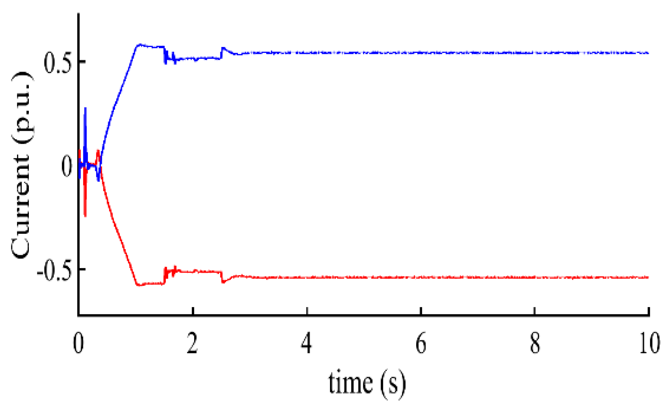
Under normal conditions, when there is no fault, DC component has a value of 0.541p.u. as shown in Figure 8. DC component reaches to a steady state in less than 3 s. Because of achieving steady state, AC components are very small. Total harmonic distortion is also negligible. Therefore, normal condition of HVDC transmission system is characterized by invariable DC component and diminishing values of AC components.
6.1.2. Positive Pole to Ground Fault (P–G Fault)
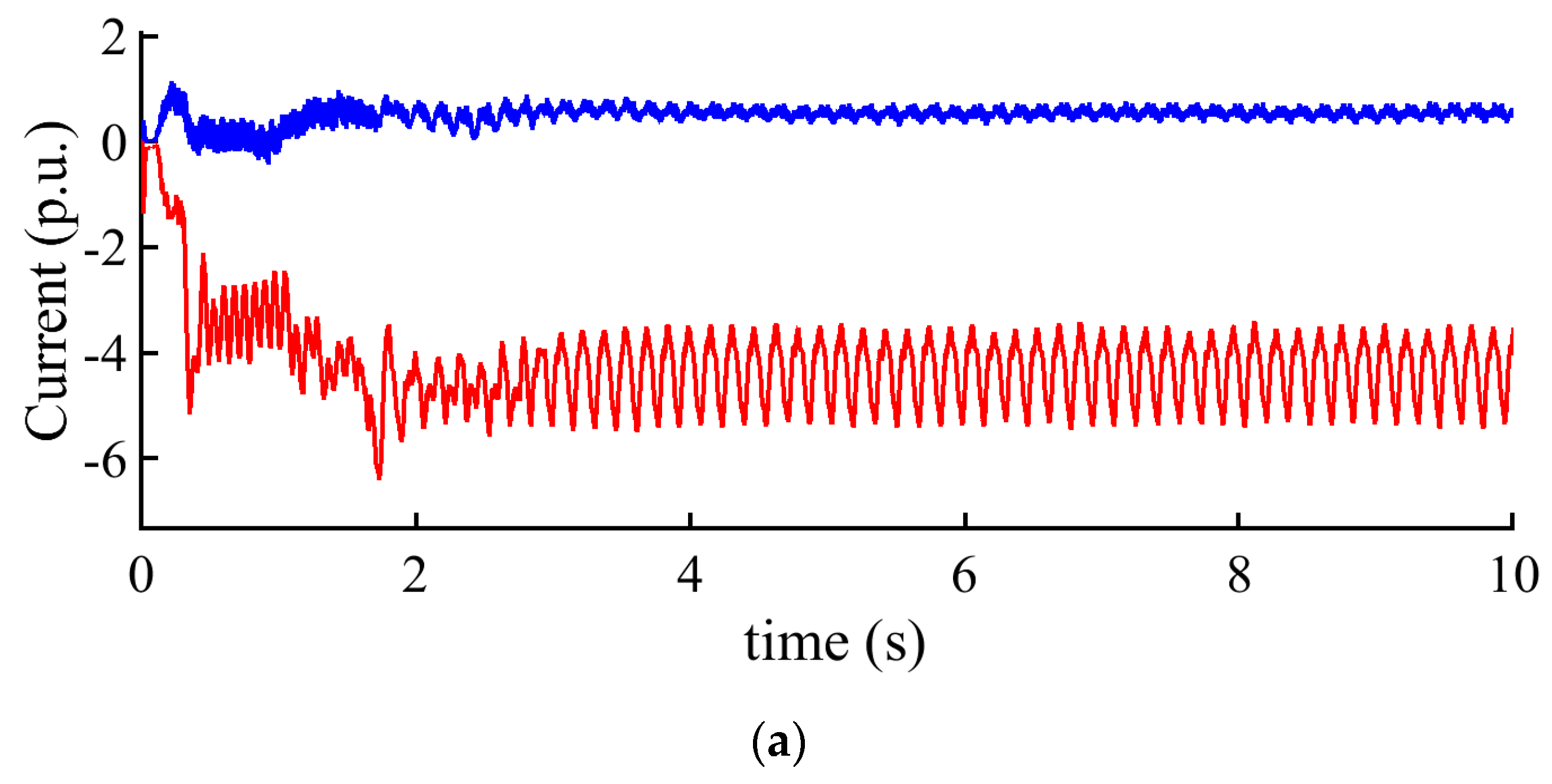
It is observed that the value of DC component is higher in positive pole to ground fault than the value of DC component under no fault condition. In addition to this, the value of total harmonic distortion (THD) is higher in the case of faulty state of HVDC system as compared to healthy state of system. These observations lead to identification of healthy and faulty states of a HVDC system. Further, in the case of positive pole to ground fault, DC component value decreases with an increase in the length of line. It is noted on positive pole that when a P–G fault occurs at converter station, DC component has value of 4.765 p.u. and at 50 km, the value of DC component is 2.887 p.u. DC component is further reduced to values of 2.321 p.u. and 1.169 p.u. at 100 km and 200 km respectively. This result leads to the estimation of fault location in a 200 km-long HVDC transmission line. Therefore, based on the values of DC component, not only faulty state of the HVDC system is identified but also location of P–G fault is estimated. P–G fault under different fault locations is shown in Figure 9.
6.1.3. Negative Pole to Ground Fault (N–G Fault)
In a similar way, negative pole to ground fault in a HVDC transmission system is identified and located by analyzing the DC component values of current at the negative pole. Higher values of DC component and THD are an indication of N–G fault in the HVDC test system. It is observed that THD value increases and DC component value decreases with the increase in the distance of fault from the sensing terminal of transmission line. N–G fault follows the same pattern of change in DC component and THD values with respect to fault location as P–G fault follows. Therefore, polarity of decrease in value of DC component with the increase in distance between fault location and fault sensing terminal aids in identification of pole to ground fault located either in positive pole or in negative pole. N–G fault under different fault locations is shown in Figure 10.
It is also realized that when one pole is subjected to fault condition, the other pole undergoes severe harmonic distortion. A sudden rise in the THD values, measured at pole opposite to faulty pole, is another indication of abnormality of HVDC test system. This realization also helps in determining the fault and its location in HVDC transmission system.
6.1.4. Positive Pole to Negative Pole Fault (P–N Fault)
In a case of pole to pole fault, it is observed that the value of DC component decreases as compared to the value of DC component under normal conditions. This decrease in the value of DC component helps in identification of faulty state of system, i.e., P–N fault.
Moreover, this observation leads to discrimination between P–G fault or N–G fault and P–N fault as a rise in the value of DC component is observed in the case of P–G fault. In addition to this, it is also noticed that the value of DC component decreases with the increase in the distance between fault point and fault sensing terminal. However, it is observed that THD values are not helpful in the determination of fault location because of no significant change in the case of P–N fault. Values of DC component are 0.3491 p.u., 0.06027 p.u., 0.0426 p.u. and 0.03009 p.u. at different fault locations of 100 m, 50 km, 100 km and 200 km respectively. It is quite significant from results that a reduction in the value of DC component is observed with the increase in the distance of fault point from converter station or fault sensing terminal. Hence, location of P–N fault in the HVDC system is identified with the values of DC component. P–N fault under different fault locations is shown in Figure 11.
6.1.5. Positive Pole to Negative Pole and Ground Fault (P–N–G Fault)
It is realized in the case of pole to pole and ground fault that value of DC component decreases as compared to the value of DC component under normal condition of HVDC test system. This decreasing value of DC component helps in recognition of faulty and healthy state of the system. Moreover, it is also noticed that the value of DC component decreases with an increase in the distance between fault location and converter station or fault sensing terminal. Values of THD are also reduced. These investigations lead to differentiation between single pole to ground fault and double pole to ground fault. However, it is not possible to distinguish between P–N fault and P–N–G fault because insignificant changes in the values of DC components and THD are observed. Therefore, some additional techniques are required to establish and to explore differences between P–N fault and P–N–G fault. P–N–G fault under different fault locations is shown in Figure 12.
It is realized from this research that the value of DC component can be the deciding factor in case of faults at greater distance from fault sensing terminals.
6.1.6. Phase to Ground Fault (Ph–G Fault)
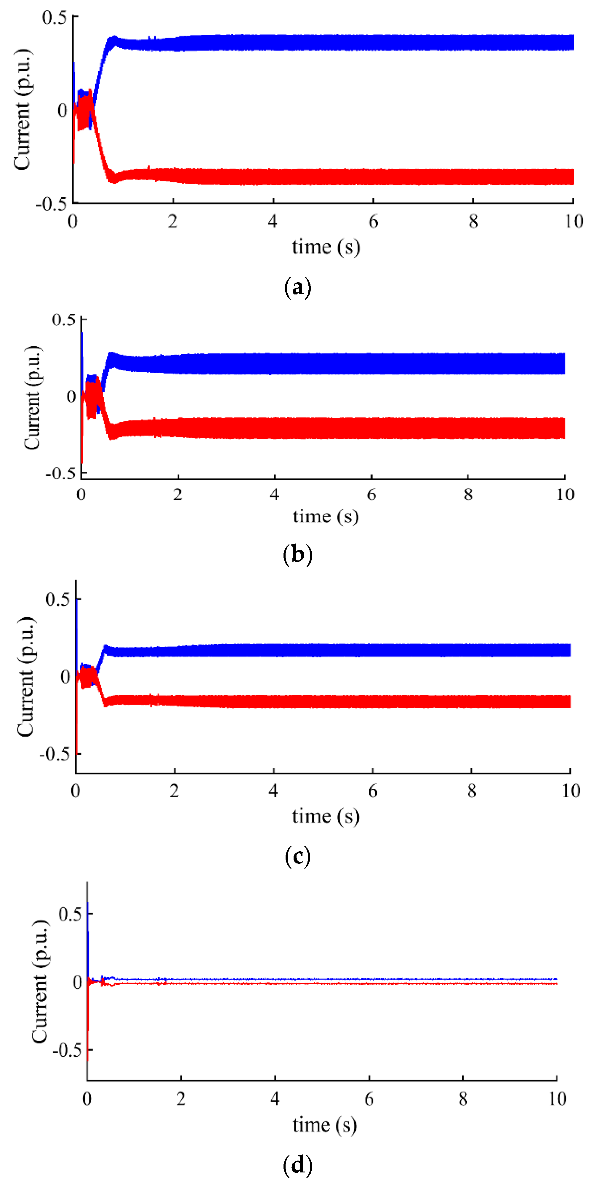
Consider a case in which different types of AC faults are applied at 200 km from fault sensing equipment located at the DC side of converter station. The value of DC component in single phase to ground AC fault is lower than the value of DC component under normal conditions. This investigation benefits in discrimination between healthy and faulty state of the system. In addition to this, this observation compels a differentiation between single pole DC fault and single-phase AC fault as the value of DC component in the case of pole to ground DC fault is higher than the value under no fault state of the test system. Further, it is noticed that THD value is increased in the case of single Ph–G AC fault. Therefore, with the decrease in DC component value and increase in THD value, Ph–G AC faults are discriminated from P–N DC fault in which a decrease in values of DC component and THD are observed. Ph–G AC fault is shown in Figure 13a.
6.1.7. Phase to Phase Fault (Ph–Ph Fault) and Phase to Phase and Ground (Ph–Ph–G Fault)
Values of DC component are also reduced in the events of phase to phase fault and phase to phase and ground fault as compared to the value of DC component under normal condition of HVDC test system. This reduction in values of DC component is clearly a manifestation of faulty state of the HVDC system. Moreover, higher values of THD are also a gesture of faulty state of test system.
It is realized from analysis that DC component and THD values in the case of Ph–Ph fault are higher than the DC component and THD values in the case of Ph–Ph–G fault. This observation leads to classification between Ph–Ph and Ph–Ph–G states of HVDC system. Ph–Ph AC fault and Ph–Ph–G AC fault are shown in Figure 13b,c.
6.1.8. Three Phase Fault (3Ph Fault) and Three Phase to Ground Fault (3Ph–G Fault)
In the case of three phase AC fault at 200 km from converter station equipped with fault sensing equipment, the value of DC component is reduced to a very small value. This outcome is a gesture of faulty state of the HVDC test system. The value of DC component is much closer to the value of DC component observed in the case of P–N and P–N–G DC fault. Therefore, THD values are employed in this case for discrimination between AC and DC faults. A higher value of THD is observed in case of 3Ph AC fault as compared to values of THD in the cases of P–N DC fault and P–N–G DC fault. 3PhAC fault and 3Ph–G AC fault are shown in Figure 13d and Figure 14.
Values of DC component and AC dominant component under different types of faults and at different locations are presented in Table 2.
6.2. Frequency Spectrum Analysis
The study of frequency spectrum of DC fault current gives an insight to determine the classification and location of DC faults in HVDC system effectively.
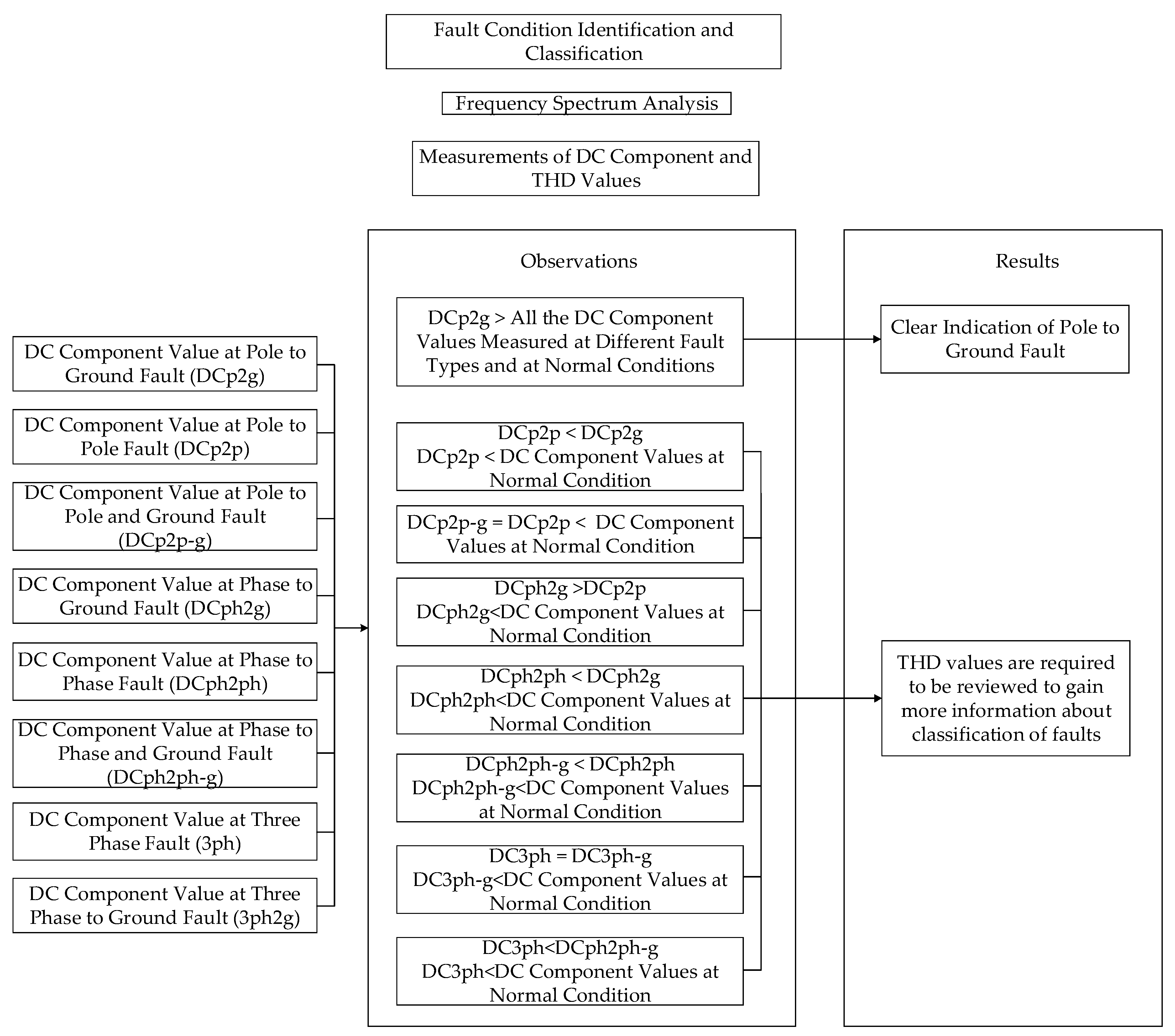
In a frequency spectrum, DC component analysis plays a symbolic role in the identification and classification of faults in the HVDC transmission system. Pole to ground faults are distinguished from other type of faults by comparing the magnitude of DC component of fault in post fault condition. The algorithm for fault identification, detection and classification based on values of DC component of fault is presented in Figure 15.
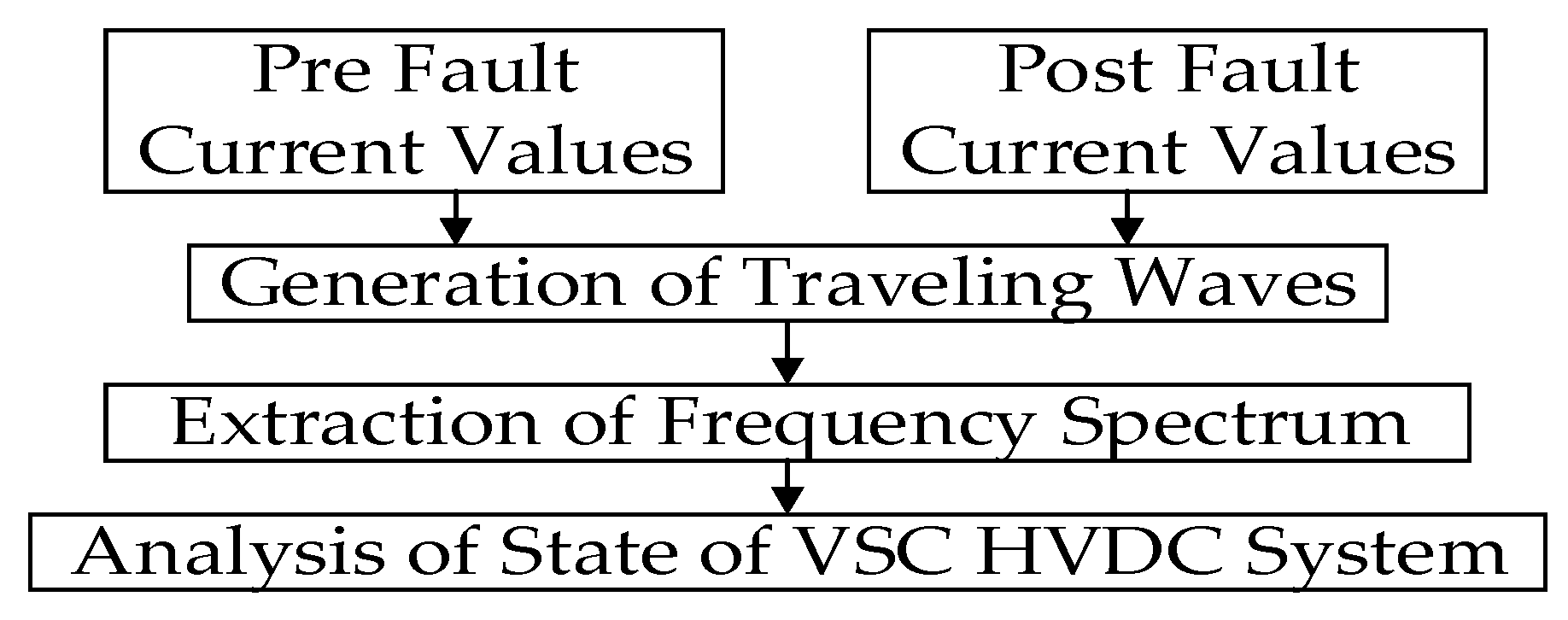
Pre-fault and post-fault values are utilized to generate traveling waves. Stepwise flow of analysis of frequency spectrum of fault current based on traveling waves is given in Figure 16. The study of frequency spectrum also depicts the AC component values of DC fault current. These AC component values also help in identification and classification of faults. Different patterns of frequency spectrum are observed at different type of faults and at different location of faults.
There are conditions of HVDC system in which DC component is not enough to estimate faults. THD values are therefore analyzed to have a clear observation of DC faults. Such conditions in which THD values are required for fault classification is presented in Figure 17. Information of total harmonic distortion (THD) also aids in discriminating between normal and faulty states and in distinguishing among different location of faults of the HVDC transmission system as shown in Figure 18.
THD values are observed under pre-fault and post-fault states of the HVDC transmission system. Comparison of THD values under pre-fault and post-fault states leads to the discrimination between P–G fault or N–G fault and P–N fault. An algorithm based on total harmonic distortion (THD) for fault estimation is presented in Figure 19.
6.2.1. Frequency Spectrum Analysis of Normal Conditions
Fast Fourier transform analysis is conducted to explore more features of this HVDC test system. Harmonics and inter-harmonics are observed in the system at different conditions of the HVDC transmission system as shown in Figure 20. It is interesting to note that amplitudes of frequency components are small. This is a manifestation of normal state of the system.
6.2.2. Frequency Spectrum Analysis of Pole to Ground Faults (P–G and N–G Faults)
In the case of pole (positive and negative) to ground DC fault, the frequency spectrum undergoes noticeable changes as compared to the frequency spectrum observed under normal state of the HVDC system. In the event of P–G fault or N–G fault at converter station, frequency spectrum is observed at positive pole for P–G fault and at negative pole for N–G fault. It is found that maximum magnitude of frequency component is 14.5 units and DC component is 15 units in the case of P–G fault and maximum amplitude of frequency component is 11 units and DC component is 14 units in the case of N–G fault. Further, frequency components are more visible in the case of N–G fault. This meaningful visibility is present in the frequency spectrum observed at any fault location throughout the entire DC line. The frequency spectrum containing DC and frequency components under different location of faults are shown in Figure 21. It is observed that the value of DC component and dominating AC component are higher in the case of P–G fault than in the case of N–G fault. This observation is found irrespective of fault location.
6.2.3. Frequency Spectrum Analysis of Pole to Pole Fault (P–N Fault)
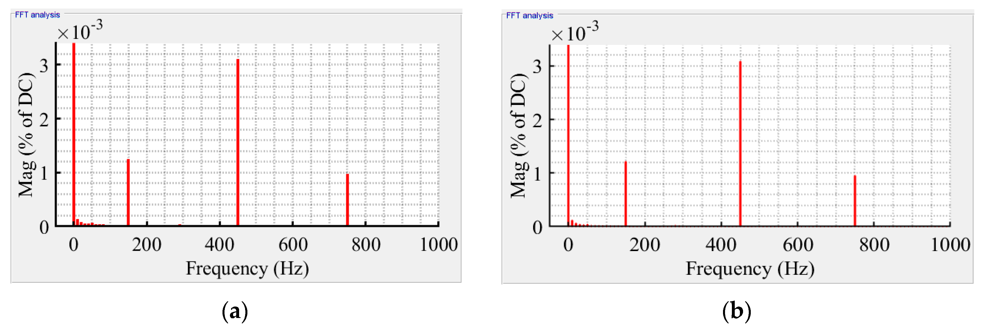
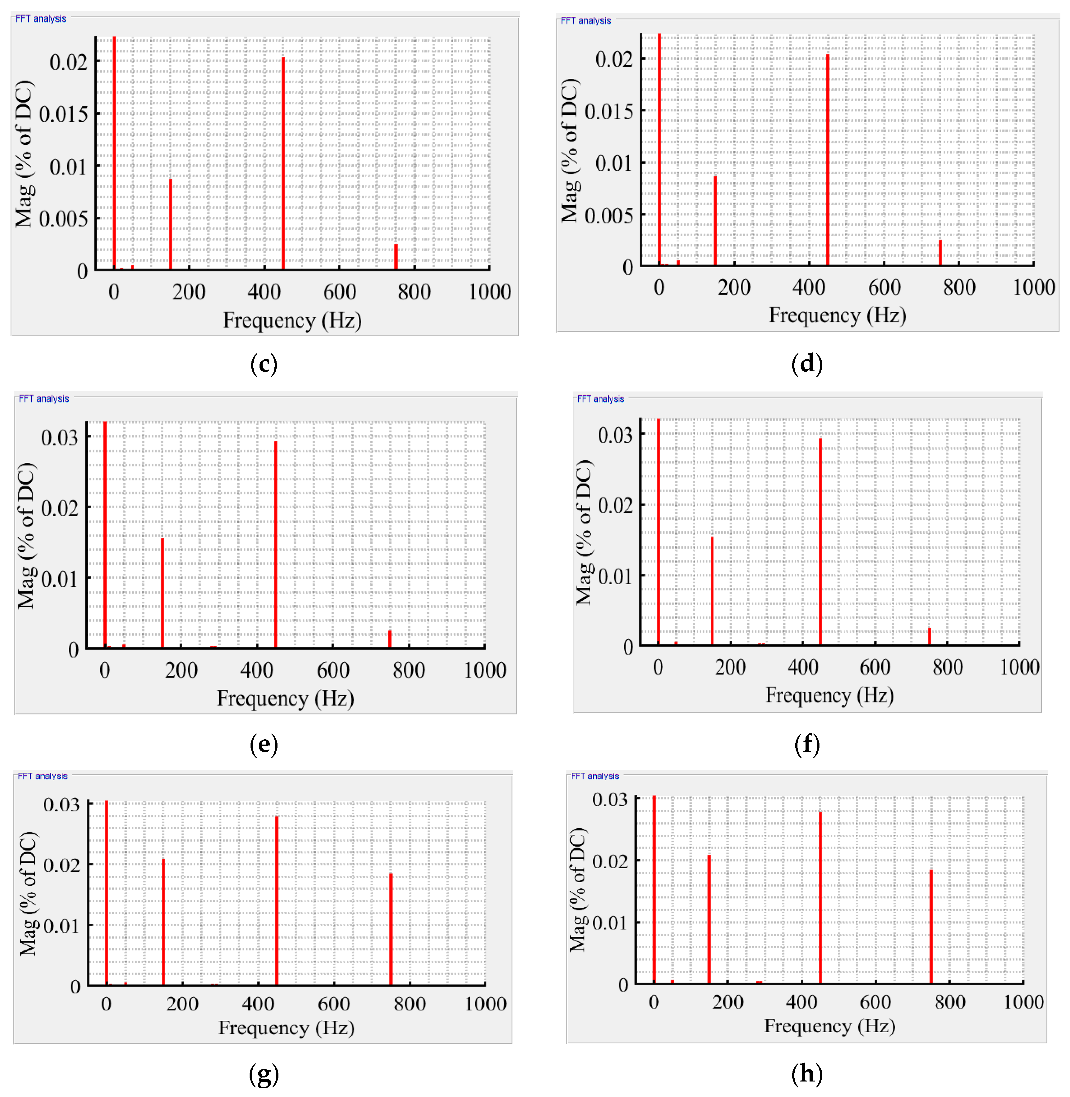
In the case of P–N faults as shown in Figure 22, frequency components, that are inter-harmonics, are not present which help in differentiating P–N faults from P–G or N–G faults. Smaller magnitudes of DC components and dominating AC components in P–N faults are shown in the frequency spectrum. This is another gesture of faulty state of the HVDC system. Only the frequency components and their harmonics are beneficial in determining the location of fault in this test system. In the frequency spectrum, it is realized at 150 Hz that magnitudes of frequency components are 0.00125 units in the case of fault at converter station, 0.008 units in the case of fault at 50 km, 0.015 units in the case of fault at 100 km and 0.021 units in the case of fault at 200 km. Rise in the magnitude of frequency component is observed with the increase in the distance between fault location and fault sensing terminal.
6.2.4. Frequency Spectrum Analysis of Pole to Pole and Ground Fault (P–N–G Fault)
In the case of P–N–G fault, decrease in the values of DC component and dominant frequency component are observed as compared to values of DC component and dominant frequency component under normal state of the HVDC test system. However, the value of frequency component increases with the increase in the distance between fault point and fault sensing terminal at converter station. Figure 23 illustrates the frequency spectrum observed at positive and negative poles under different fault locations.
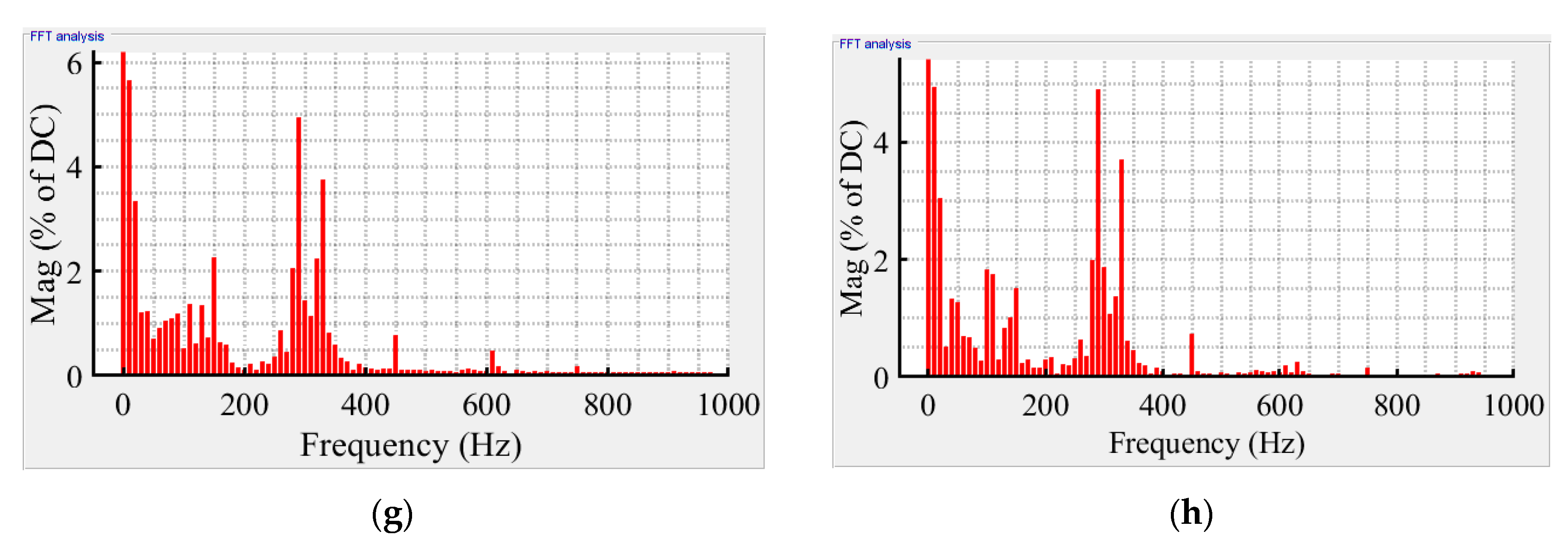
6.2.5. Frequency Spectrum Analysis of Three Phase Faults (3Ph and 3Ph–G Faults)
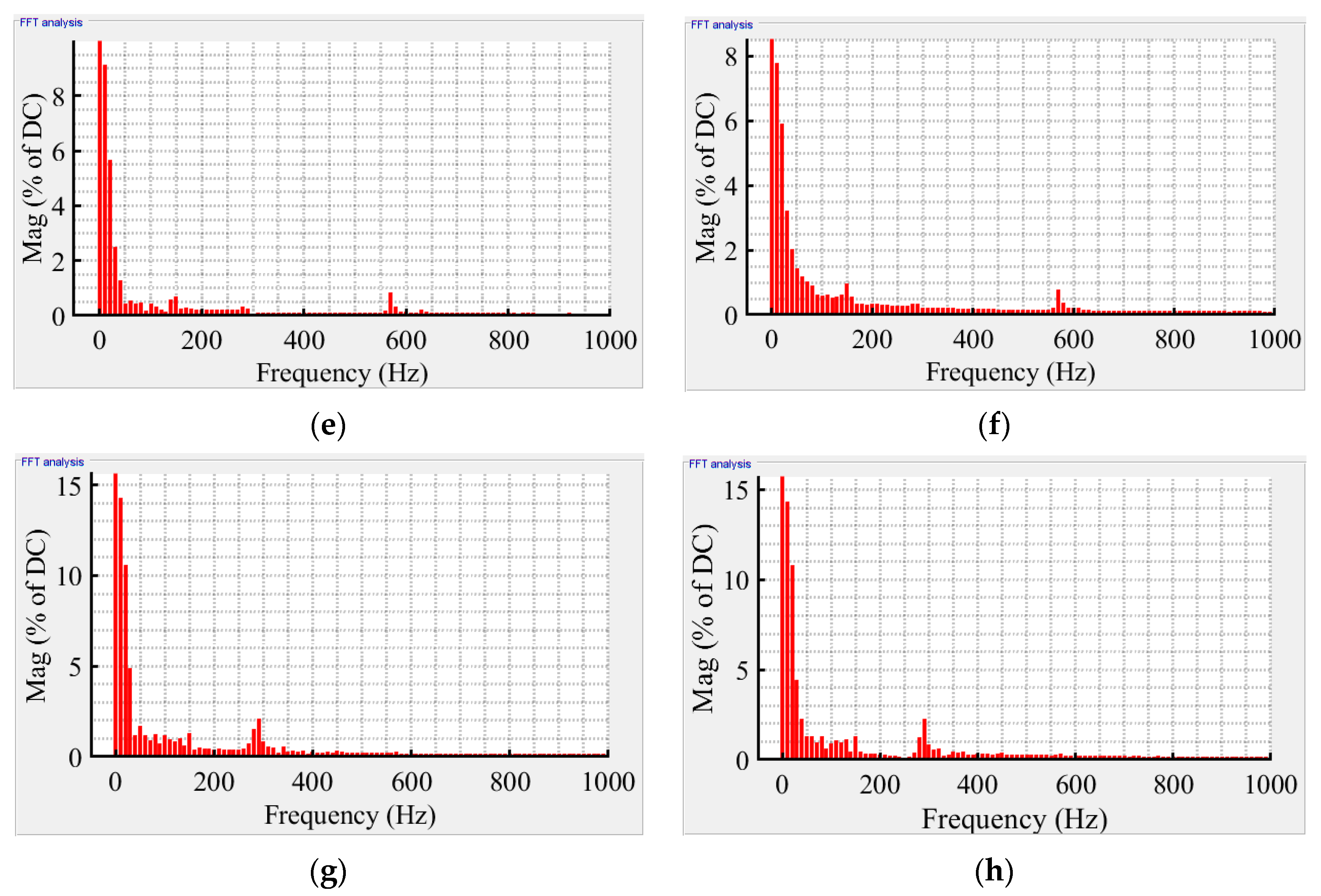
In the events of three phase faults, traveling wave of fault current is rich in harmonics and inter-harmonics as shown in Figure 24g,h. In other words, transient nature is more observable in three phase faults as compared to single-phase and two-phase faults. These harmonics and inter-harmonics are smaller in magnitude. As a result, THD values are also small in three-phase faults. The value of DC component is small as compared to values of DC component in other AC faults. These indications create a difference from other AC fault conditions.
Hence, analysis of the frequency spectrum not only depicts the state of the HVDC transmission system but also exhibits a differentiation among different faults of the HVDC transmission system. Figure 25 presents a classification of faults based on the values of THD obtained from analysis of the frequency spectrum.
6.3. Discrimination of AC Faults
In the case of AC faults, magnitudes of DC component and dominating frequency component increase to very large values as compared to values of DC component and dominating frequency component of normal state of the HVDC test system as shown in Figure 23. Further, it is observed from frequency spectrum that the value of DC component and dominating frequency component are lower for Ph–G fault as compared to Ph–Ph fault. Moreover, DC component and dominating AC component in the case of phase to phase fault are lower as compared to Ph–Ph–G fault. These investigations are advantageous in finding the type of fault occurred in the HVDC test system.
6.4. Significance of Second Harmonics
It is observed that in the events of AC faults, DC component, AC fundamental component and its second harmonics are dominant. These findings are beneficial for discrimination between AC and DC faults occurred at converter stations.
6.5. Benefits of Frequency Spectrum Analysis
Following are the benefits associated with frequency spectrum analysis of states of the HVDC transmission system.
- In the case of faults at converter stations (AC or DC faults), there is a possibility that current flowing in the DC line under DC or AC fault condition has a similar characteristics curve. Therefore, there is a need to explore more about magnitude of DC component and its dominant AC components. Fast Fourier transform is conducted and frequency spectrum is analyzed as shown in Figure 20, Figure 21, Figure 22, Figure 23 and Figure 24 under different states (normal, pole to ground fault, phase to ground fault and three phase fault) and at different locations of the HVDC system. Frequency based analysis is valuable for differentiating between faulty states of HVDC system. In this research, it is found that DC component under DC fault has a much higher value than under AC faults. Transient nature is more observable in three phase AC faults as compared to DC faults. Therefore, this result plays a significant role in determining the faults at AC or DC side of converter station. Further, not only relaying strategy can be determined from this result but also the nature of primary and backup protection can be predicted.
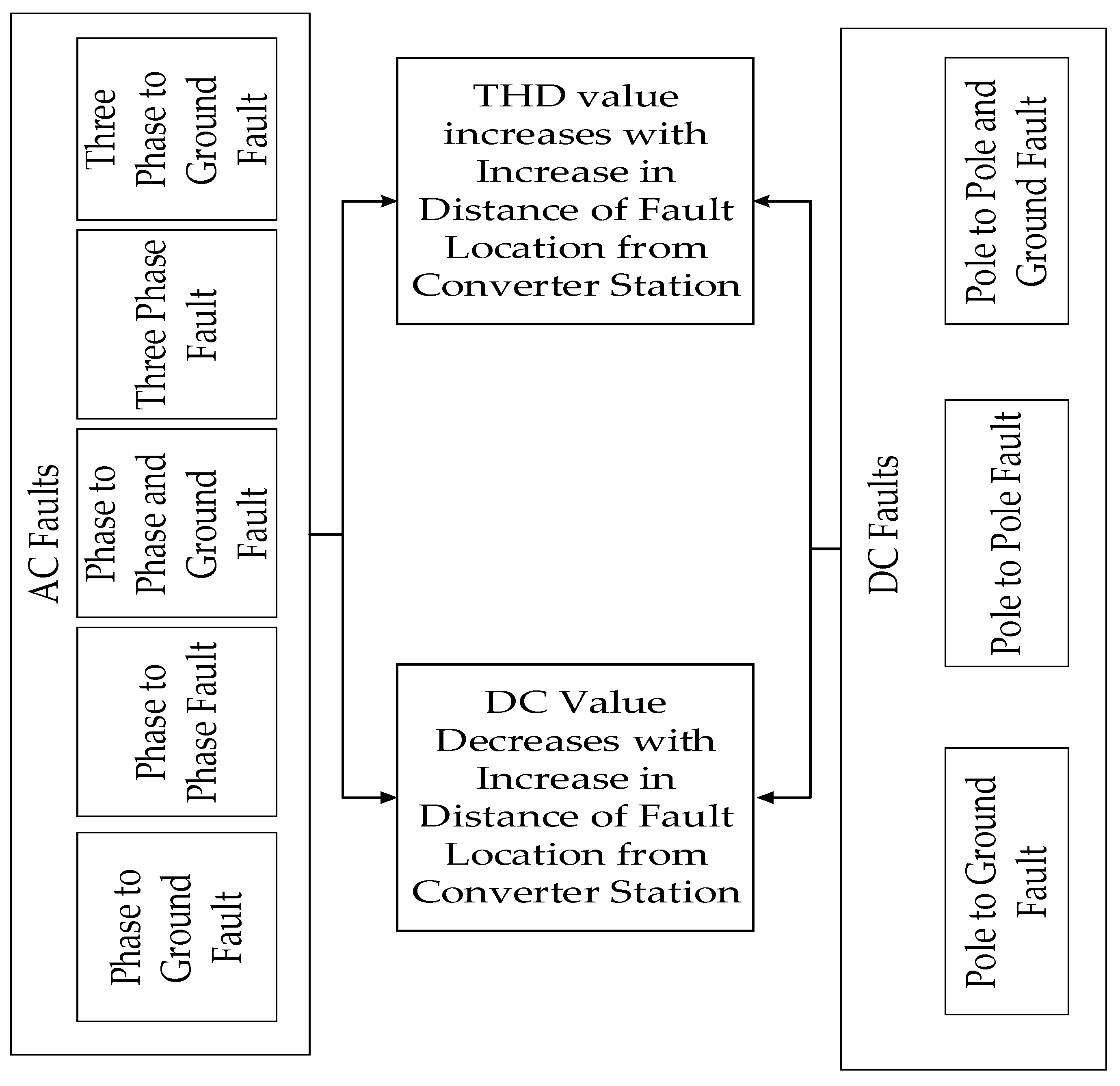
- Locations of faults are identified by comparing the magnitude of DC component of DC fault current. In the frequency spectrum, it is noted that DC value decreases with the increase in distance from converter station but THD value increases with the increase in distance from converter station. Hence, it is concluded that the spectrum of frequency components is utilized for classification of fault with respect to location of fault, particularly in a case when the fault is not readily distinguished from values of DC fault current. The relationship of location of fault with respect to DC value of fault current and THD values is presented in Figure 26.
- This analysis is found beneficial for determining the states of the HVDC system. In a test system, it is observed that phase to ground fault has same characteristics curve of DC fault current as that of normal state of the system. In such cases, it is not easy to determine the state of the system. However, with the help of Fast Fourier transform, fundamental component and harmonics reveal the information about the state of system. Phase to ground fault hasa characteristics curve which is rich in harmonics as compared to DC current flowing under normal state of the system. Moreover, it helps to determine the forward (DC faults) and backward faults (AC faults) of converter stations.
6.6. Performance Comparison of Fault Location Estimation Techniques
In this proposed research, a HVDC test system is analyzed comprehensively under different conditions of fault. It is found that fault is identified, classified and located promptly and easily by this technique. Table 3 provides a detailed comparison of fault estimation techniques on the basis of different technical factors associated with traveling waves.
7. Conclusions
In this research paper, traveling wave-based methods for fault estimation in a HVDC transmission system are reviewed. Limitations of traveling wave-based techniques like difficulties in detection of wave front, compromised propagation velocity because of transmission line parameters, complexity of phase modal transformation and effects of transition resistance are presented. It is concluded that there is a need of additional approaches like wavelet transform, artificial neural networks, machine learning, correlation and similarity measures, discriminant analysis, etc., along with the conventional traveling wave-based method for accurate estimation of fault in HVDC transmission systems. Only the parameters like velocity propagation and natural frequency are not enough for better estimation of fault.
Further, VSC-based HVDC transmission systems are analyzed to develop a protection scheme based on DC component, dominating AC component and total harmonic distortion of traveling wave of DC fault current. Different types of DC and AC faults held at different locations in HVDC transmission system are discriminated progressively with this protection scheme. Therefore, performance of traveling wave-based proposed fault estimation technique is validated on the basis of its successful identification, classification and estimation of location of faults. Moreover, fast Fourier transform is also performed to analyze the change in frequency components with the change in fault types. It is concluded that DC currents change rapidly in the case of DC faults while there is no significant change in DC currents in the case of AC faults. Therefore, the frequency spectrum of traveling wave gives an insight into the identification of the type of AC and DC faults. In addition to this, analysis of frequency spectrum is beneficial for distinguishing between backward (AC)faults and forward (DC) faults at converter stations which remained an unsolved problem for many years. This consequence is a major breakthrough in upgrading relaying schemes for HVDC systems. This proposed technique also helps in identification of effects of AC faults on HVDC systems. This intuition provides a provision of extension to multi-terminal systems and interconnection to renewable energy technology without the fear of instability and black outs.
Funding
This research received no external funding.
Conflicts of Interest
The author declares no conflict of interest.
References
- Fairley, P. DC versus AC: The second war of currents has already begun. IEEE Power Energy Mag. 2012, 10, 102–104. [Google Scholar] [CrossRef]
- Reed, G. DC technologies—Solutions to electric power system advancements. IEEE Power Energy Mag. 2012, 10, 10–17. [Google Scholar] [CrossRef]
- Adapa, R. High-wire act: HVDC technology: The state of the art. IEEE Power Energy Mag. 2012, 10, 18–29. [Google Scholar] [CrossRef]
- Padiyar, K.R. HVDC Power Transmission Systems: Technology and System Interactions; Wiley: Hoboken, NJ, USA, 1990. [Google Scholar]
- Nanayakkara, O.M.K.K.; Rajapakse, A.D.; Wachal, R. Location of DC line faults in conventional HVDC systems with segments of cables and overhead lines using terminal measurements. IEEE Trans. Power Del. 2012, 27, 279–288. [Google Scholar] [CrossRef]
- Nanayakkara, O.M.K.K.; Rajapakse, A.D.; Wachal, R. Traveling wave based line fault location in star-connected multi-terminal HVDC systems. IEEE Trans. Power Del. 2012, 27, 2286–2294. [Google Scholar] [CrossRef]
- Dewe, M.B.; Sankar, S.; Arrillaga, J. The application of satellite time references to HVDC fault location. IEEE Trans. Power Del. 1993, 8, 1295–1302. [Google Scholar] [CrossRef]
- Ping, C.; Bingyin, X.; Jing, L.; Yaozhong, G. Modern traveling wave based fault location techniques for HVDC transmission lines. Trans. Tianjin Univ. 2008, 14, 139–143. [Google Scholar]
- Swetha, A.; Murthy, P.K.; Sujatha, N.; Kiran, Y. A novel technique for the location of fault on a HVDC transmission line. J. Eng. Appl. Sci. 2011, 6, 62–67. [Google Scholar]
- Ando, M.; Schweitzer, E.O.; Baker, R.A. Development and field-data evaluation of single-end fault locator for two-terminal HVDC transmission lines-part 2: Algorithm and evaluation. IEEE Trans. Power App. Syst. 1985, PAS-104, 3531–3537. [Google Scholar] [CrossRef]
- Sachdev, M.S.; Wood, H.C.; Johnson, N.G. Kalman filtering applied to power system measurements for relaying. IEEE Trans. Power App. Syst. 1985, 104, 3565–3573. [Google Scholar] [CrossRef]
- Das, S.; Santoso, S.; Gaikwad, A.; Patel, M. Impedance-based fault location in transmission networks: Theory and application. IEEE Access 2014, 2, 537–557. [Google Scholar] [CrossRef]
- Dzienis, C.; Yelgin, Y.; Washer, M.; Maun, J.-C. Accurate impedance based fault location algorithm using communication between protective relays. In Proceedings of the 2015 Modern Electric Power Systems (MEPS), Wroclaw, Poland, 6–9 July 2015. [Google Scholar]
- Bustamante-Mparsakis, X.; Maun, J.C.; Dzienis, C.; Jurisch, A. Travelling wave fault location based on pattern recognition. In Proceedings of the 2017 IEEE Manchester PowerTech, Manchester, UK, 18–22 June 2017. [Google Scholar]
- Lopes, F.; Dantas, K.; Silva, K.; Costa, F.B. Accurate Two-Terminal Transmission Line Fault Location Using Traveling Waves. IEEE Trans. Power Del. 2017, 33, 873–880. [Google Scholar] [CrossRef]
- Sachdev, M.S.; Aggarwal, R. A technique for estimating transmission line fault locations from digital impedance relay measurements. IEEE Trans. Power Del. 1988, 3, 121–129. [Google Scholar] [CrossRef]
- Eriksson, L.; Saha, M.M.; Rockefeller, G.D. An accurate fault locator with compensation for apparent reactance in the fault resistance resulting from remote-end infeed. IEEE Trans. Power Appar. Syst. 1985, 104, 423–436. [Google Scholar] [CrossRef]
- Johns, A.T.; Jamali, S. Accurate fault location technique for power transmission lines. IEE Proc. Part C 1990, 137, 395–402. [Google Scholar] [CrossRef]
- Yuan, L.; Ning, K. Fault-location algorithms without utilizing line parameters based on the distributed parameter line model. IEEE Trans. Power Del. 2009, 24, 579–584. [Google Scholar] [CrossRef]
- Xu, H.; Song, G. A novel traveling wave head identification method in VSC-HVDC based on parameter identification. In Proceedings of the 2015 5th International Conference on Electric Utility Deregulation and Restructuring and Power Technologies (DRPT), Changsha, China, 26–29 November 2015. [Google Scholar]
- Song, G.; Cai, X.; Gao, S.; Suonan, J.; Li, G. Natural frequency based protection and fault location for VSC-HVDC transmission lines. In Proceedings of the 2011 International Conference on Advanced Power System Automation and Protection, Beijing, China, 16–20 October 2011. [Google Scholar]
- He, Z.Y.; Liao, K.; Li, X.P.; Lin, S.; Yang, J.W.; Mai, R.K. Natural Frequency-Based Line Fault Location in HVDC Lines. IEEE Trans. Power Del. 2014, 29, 851–859. [Google Scholar] [CrossRef]
- Chanda, N.K.; Fu, Y. ANN-based fault classification and location in MVDC shipboard power systems. In Proceedings of the 2011 North American Power Symposium, Boston, MA, USA, 4–6 August 2011. [Google Scholar]
- Rajesh, K.; Yadaiah, N. Fault Identification Using Wavelet Transform. In Proceedings of the 2005 IEEE/PES Transmission and Distribution Conference and Exhibition: Asia and Pacific, Dalian, China, 18 August 2005; pp. 1–6. [Google Scholar]
- Li, Y.; Gong, Y.F.; Jiang, B. A novel traveling-wave-based directional protection scheme for MTDC grid with inductive DC terminal. Electr. Power Syst. Res. 2018, 157, 83–92. [Google Scholar] [CrossRef]
- Liu, K.; Yang, X.; Li, Y.; Wang, J. Study of protection for serial multi-terminal DC grids. J. Int. Counc. Electr. Eng. 2018, 8, 71–77. [Google Scholar] [CrossRef]
- Crossley, P.A.; McLaren, P. Distance protection based on traveling waves. IEEE Trans. Power App. Syst. 1983, 102, 2971–2983. [Google Scholar] [CrossRef]
- Shehab-Eldin, E.; McLaren, P. Traveling wave distance protection-problem areas and solutions. IEEE Trans. Power Del. 1986, 1, 894–902. [Google Scholar]
- McLaren, P.; Rajendra, S.; Shehab-Eldin, E.; Crossley, P. Ultra high speed distance protection based on traveling waves. In Proceedings of the IEE Conference Publication No. 249 ‘Developments in Power System Protection’, London, UK, April 1985; pp. 106–110. [Google Scholar]
- Christopoulos, C.; Thomas, D.; Wright, A. Scheme based on traveling waves, for the protection of major transmission lines. IEE Proc. Part C 1988, 135, 63–73. [Google Scholar]
- Christopoulos, C.; Thomas, D.; Wright, C. Signal processing and discriminating techniques incorporated in a protective scheme based on traveling waves. IEE Proc. Part C 1989, 136, 279–288. [Google Scholar]
- Dutta, P.; Duttagupta, P. Microprocessor-based UHS distance relaying and fault locating algorithms for EHV transmission lines. In Proceedings of the International Conference on Power System Protection, Singapore, September 1989; pp. 315–337. [Google Scholar]
- Dommel, H.W.; Michels, J.M. High speed relaying using traveling wave transient analysis. In Proceedings of the IEEE PES Winter Meeting, Paper A, New York, NY, USA, 29 January–3 February 1978. [Google Scholar]
- Ancell, G.B.; Pahalawaththa, C. Maximum likelihood estimation of fault location on transmission lines using traveling waves. IEEE Trans.Power Del. 1994, 9, 680–689. [Google Scholar]
- Bewley, L.V. Traveling Waves on Transmission Systems, 2nd ed.; Dover Publications Inc.: New York, NY, USA, 1963. [Google Scholar]
- Tang, Y.; Chen, H.; Wang, H.; Dai, F. Transmission line models used in traveling wave studies. In Proceedings of the Transmission Distribution Conference, New Orleans, LA, USA, 11–16 April 1999; Volume 2, pp. 797–803. [Google Scholar]
- Chen, P.; Xu, B.; Li, J. A traveling wave based fault locating system for HVDC transmission lines. In Proceedings of the International Conference on Power System Technology, Chongqing, China, 22–26 October 2006; pp. 1–4. [Google Scholar]
- Radford, T.W. HVDC line fault locator upgrade. In Proceedings of the HVDC System Operating Conference, Winnipeg, MB, Canada, 15–17 September 1987; pp. 189–200. [Google Scholar]
- Shang, L.; Herold, G.; Jaeger, J.; Krebs, R.; Kumar, A. High-speed fault identification and protection for HVDC line using wavelet technique. In Proceedings of the IEEE Porto Power Tech Proceedings, Porto, Portugal, 10–13 September 2001; pp. 1–5. [Google Scholar]
- Evrenosoglu, C.Y.; Abur, A. Traveling wave based fault location for teed circuits. IEEE Trans. Power Del. 2005, 20, 1115–1121. [Google Scholar] [CrossRef]
- Magnago, F.H.; Abur, A. Fault location using wavelets. IEEE Trans. Power Del. 1998, 13, 1475–1480. [Google Scholar] [CrossRef]
- Nanayakkara, K.; Rajapakse, A.D.; Wachal, R. Fault location in extra HVDC transmission line using continuous wavelet transform. In Proceedings of the IPST Conference, Delft, The Netherlands, 14–17 June 2011. [Google Scholar]
- Gale, P.F.; Taylor, P.V.; Naidoo, P.; Hitchin, C.; Clowes, D. Traveling wave fault locator experience on Eskom’s transmission network. In Proceedings of the Seventh International Conference on Developments in Power System Protection, Amsterdam, The Netherlands, 9–12 April 2001; Volume 14, pp. 327–330. [Google Scholar]
- Kumar, K.P. Fault diagnosis for an HVDC system: A feasibility study of an expert system application. Electric Power Syst. Res. 1988, 14, 83–89. [Google Scholar]
- Shultz, R.D.; Gonzales, R.F. Operating characteristics of an HVDC multi terminal transmission line under single pole faulted conditions and high resistance earth return. Electric Power Syst. Res. 1986, 10, 103–111. [Google Scholar] [CrossRef]
- Swift, G.W. The Spectra of Fault-Induced Transients. IEEE Trans. Power App. Syst. 1979, PAS-98, 940–947. [Google Scholar] [CrossRef]
- Styvaktakis, E.; Bollen, M.H.J.; Gu, H.Y. A fault location technique using high frequency fault clearing transients. IEEE Power Engg. Rev. 1999, 19, 58–60. [Google Scholar] [CrossRef]
- Li, Y.L.; Zhang, Y.; Ma, Z.Y. Fault location method based on the periodicity of the transient voltage traveling wave. In Proceedings of the IEEE Region 10 Conference, Chiang Mai, Thailand, 24 November 2004; Volume 3, pp. 389–392. [Google Scholar]
- Zou, Y.; Wang, X.; Zhang, H.; Liu, C.; Zhou, Q.; Zhu, W. Traveling-wave based fault location with high grounding resistance for HVDC transmission lines. In Proceedings of the 2016 IEEE PES Asia-Pacific Power and Energy Engineering Conference (APPEEC), Xi’an, China, 25–28 October 2016; pp. 1651–1655. [Google Scholar]
- Leite, E.J.S.; Lopes, F.V. Traveling wave-based fault location formulation for hybrid lines with two sections. In Proceedings of the2017 Workshop on Communication Networks and Power Systems (WCNPS), Brasília, Brazil, 16–17 November 2017; pp. 1–4. [Google Scholar]
- Giovanni, M. Transmission Lines and Lumped Circuits; Academic Press: San Diego, CA, USA, 2001; pp. 64–84. [Google Scholar]
- Zhang, S.; Zou, G.; Huang, Q.; Gao, H. A traveling-wave-based fault location scheme for MMC-based multi-terminal DC grids. Energies 2018, 11, 401. [Google Scholar] [CrossRef]
- Xu, Y.; Liu, J.; Jin, W.; Fu, Y.; Yang, H. Fault Location Method for DC Distribution Systems Based on Parameter Identification. Energies 2018, 11, 1983. [Google Scholar] [CrossRef]
- Liu, K.; Huai, Q.; Qin, L.; Zhu, S.; Liao, X.; Li, Y.; Ding, H. Enhanced Fault Current-Limiting Circuit Design for a DC Fault in a Modular Multilevel Converter-Based High-Voltage Direct Current System. Appl. Sci. 2019, 9, 1661. [Google Scholar] [CrossRef]
- Lan, T.; Li, Y.; Duan, X.; Zhu, J. Simplified Analytic Approach of Pole-to-Pole Faults in MMC-HVDC for AC System Backup Protection Setting Calculation. Energies 2018, 11, 264. [Google Scholar] [CrossRef]
- Muzzammel, R. Machine Learning Based Fault Diagnosis in HVDC Transmission Lines. In Intelligent Technologies and Applications; Springer: Singapore, 2019; Volume 932. [Google Scholar]
- Hao, W.; Mirsaeidi, S.; Kang, X.; Dong, X.; Tzelepis, D. A novel traveling-wave-based protection scheme for LCC-HVDC systems using teager energy operator. Int. J. Electr. Power Energy Syst. 2018, 99, 474–480. [Google Scholar] [CrossRef]
- Jin, H.; Lu, B.; Tan, F.; Chen, P.; Si, W.; Yang, L. Application of distributed traveling wave ranging technology in fault diagnosis of HVDC transmission line. IOP Conf. Ser.: Earth Environ. Sci. 2018, 186, 012039. [Google Scholar] [CrossRef]
- Ikhide, M.; Tennakoon, S.; Griffiths, A.; Subramanian, S.; Ha, H.A. Transient based protection technique for future DC grids utilising travelling wave power. J. Eng. 2018, 2018, 1267–1273. [Google Scholar] [CrossRef]
- Jiang, L.; Chen, Q.; Huang, W.; Wang, L.; Zeng, Y.; Zhao, P. Pilot protection based on amplitude of directional travelling wave for voltage source converter-high voltage direct current (VSC-HVDC) transmission lines. Energies 2018, 11, 2021. [Google Scholar] [CrossRef]
- Padiyar, K.R.; Prabhu, N. Modelling, control design and analysis of VSC based HVDC transmission system. In Proceedings of the International Conference on Power System Technology, Singapore, 21–24 November 2004; Volume 1, pp. 774–779. [Google Scholar]
- Stan, A.I. Control of VSC-Based HVDC Transmission System for Offshore Wind Power Plants. Master’s Thesis, Aalborg University, Aalborg, Denmark, 2010. [Google Scholar]
- Bajracharya, C. Control of VSC-HVDC for wind power. Master’s Thesis, Norwegian University of Science and Technology, Trondheim, Norway, 2008. [Google Scholar]
Figure 1.
Traveling wave.

Figure 2.
Frequency spectrum of traveling wave at the instant of fault.

Figure 3.
Route of reflection of traveling wave at the time of fault over HVDC transmission line.

Figure 4.
Equivalent model of double conductor HVDC transmission line.

Figure 5.
Voltage source converter (VSC) based HVDC test system.

Figure 6.
Matlab/Simulink model of VSC–HVDC transmission system.

Figure 7.
Scheme of fault estimation in HVDC transmission system.

Figure 8.
Current waveform of positive and negative pole of a 200 km-long HVDC transmission line system under normal conditions.
Figure 8.
Current waveform of positive and negative pole of a 200 km-long HVDC transmission line system under normal conditions.

Figure 9.
Current waveform of positive and negative pole of a 200 km-long HVDC transmission system under positive pole to ground fault at (a) converter station; (b) 50 km; (c) 100 km; (d) 200 km.
Figure 9.
Current waveform of positive and negative pole of a 200 km-long HVDC transmission system under positive pole to ground fault at (a) converter station; (b) 50 km; (c) 100 km; (d) 200 km.

Figure 10.
Current waveform of positive and negative pole of 200 km-long HVDC transmission system under negative pole to ground fault at (a) converter station; (b) 50 km; (c) 100 km; (d) 200 km.
Figure 10.
Current waveform of positive and negative pole of 200 km-long HVDC transmission system under negative pole to ground fault at (a) converter station; (b) 50 km; (c) 100 km; (d) 200 km.


Figure 11.
Current waveform of positive and negative pole of a 200 km-long HVDC transmission system under pole to pole fault at (a) converter station; (b) 50 km; (c) 100 km; (d) 200 km.
Figure 11.
Current waveform of positive and negative pole of a 200 km-long HVDC transmission system under pole to pole fault at (a) converter station; (b) 50 km; (c) 100 km; (d) 200 km.

Figure 12.
Current waveform of positive and negative pole of 200 km-long HVDC transmission system under pole to pole and ground fault at (a) converter station; (b) 50 km; (c) 100 km; (d) 200 km.
Figure 12.
Current waveform of positive and negative pole of 200 km-long HVDC transmission system under pole to pole and ground fault at (a) converter station; (b) 50 km; (c) 100 km; (d) 200 km.

Figure 13.
Current waveform of positive and negative pole of 200 km-long HVDC transmission system under (a) phase to ground AC fault at 200 km; (b) phase to phase AC fault at 200 km; (c) double phase to ground AC fault at 200 km; (d) three phase AC fault at 200 km.
Figure 13.
Current waveform of positive and negative pole of 200 km-long HVDC transmission system under (a) phase to ground AC fault at 200 km; (b) phase to phase AC fault at 200 km; (c) double phase to ground AC fault at 200 km; (d) three phase AC fault at 200 km.

Figure 14.
Current waveform of positive and negative pole of 200 km-long HVDC transmission system under three phase to ground AC fault at 200 km.
Figure 14.
Current waveform of positive and negative pole of 200 km-long HVDC transmission system under three phase to ground AC fault at 200 km.

Figure 15.
DC component analysis for fault estimation in VSC–HVDC transmission system.

Figure 16.
Step wise flow for analysis of state of HVDC system.

Figure 17.
Requirement of THD values for fault estimation in VSC–HVDC transmission system.

Figure 18.
Analysis of frequency spectrum of traveling waves for classification and location of fault in VSC–HVDC transmission system.
Figure 18.
Analysis of frequency spectrum of traveling waves for classification and location of fault in VSC–HVDC transmission system.

Figure 19.
Total harmonic distortion for DC fault classification in VSC–HVDC transmission system.

Figure 20.
Fast Fourier transform analysis of current waveform of 200 km-long HVDC transmission line system under normal conditions (a) at positive pole; (b) at negative pole.
Figure 20.
Fast Fourier transform analysis of current waveform of 200 km-long HVDC transmission line system under normal conditions (a) at positive pole; (b) at negative pole.

Figure 21.
Fast Fourier transform analysis of current waveform of a 200 km-long HVDC transmission line system under (a) positive pole to ground fault at converter station; (b) negative pole to ground fault at converter station; (c) positive pole to ground fault at 50 km; (d) negative pole to ground fault at 50 km; (e) positive pole to ground fault at 100 km; (f) negative pole to ground fault at 100 km; (g) positive pole to ground fault at 200 km; (h) negative pole to ground fault at 200 km.


Figure 22.
Fast Fourier transform analysis of current waveform of a 200 km-long HVDC transmission line system conducted at (a) positive pole under pole to pole fault occurred at converter station; (b) negative pole under pole to pole fault occurred at converter station; (c) positive pole under pole to pole fault occurred at 50 km; (d) negative pole under pole to pole fault occurred at 50 km; (e) positive pole under pole to pole fault occurred at 100 km; (f) negative pole under pole to pole fault occurred at 100 km; (g) positive pole under pole to pole fault occurred at 200 km; (h) negative pole under pole to pole fault occurred at 200 km.


Figure 23.
Fast Fourier transform analysis of current waveform of a 200 km-long HVDC transmission line system conducted at (a) positive pole under pole to pole and ground fault occurred at converter station; (b) negative pole under pole to pole and ground fault occurred at converter station; (c) positive pole under pole to pole and ground fault occurred at 50 km; (d) negative pole under pole to pole and ground fault occurred at 50 km; (e) positive pole under pole to pole and ground fault occurred at 100 km; (f) negative pole under pole to pole and ground fault occurred at 100 km; (g) positive pole under pole to pole and ground fault occurred at 200 km; (h) negative pole under pole to pole and ground fault occurred at 200 km.

Figure 24.
Fast Fourier transform analysis of current waveform of a 200 km-long HVDC transmission line system conducted at (a) positive pole under phase to ground AC fault occurred at 200 km; (b) negative pole under phase to ground AC fault occurred at 200 km; (c) positive pole under phase to phase and ground AC fault occurred at 200 km; (d) negative pole under phase to phase and ground AC fault occurred at 200 km; (e) positive pole under phase to phase AC fault occurred at 200 km; (f) negative pole under phase to phase AC fault occurred at 200 km; (g) positive pole under three phase AC fault occurred at 200 km; (h) negative pole under three phase AC fault occurred at 200 km.


Figure 25.
Classification of faults on the basis of THD values in VSC–HVDC transmission system.

Figure 26.
Relationship of location of faults with respect to DC value and THD value in VSC–HVDC transmission system.
Figure 26.
Relationship of location of faults with respect to DC value and THD value in VSC–HVDC transmission system.


Table 1.
Values of VSC–HVDC transmission system.
| Parameters | Grid Station I | Grid Station II |
|---|---|---|
| Voltage (kV) | 230 | 230.100 |
| Frequency (Hz) | 50 | 50 |
| Power (MVA) | 2000 | 2000 |
| Voltage Source Converter (MVA) | 200 | 200 |
| Phase Reactor (p.u.) | 0.15 | 0.15 |
| Rectifier/Inverter | Rectifier | Inverter |
| Three Phase Fault | No | Yes |
| DC Fault | No | Yes |
Table 2.
Values of DC component and AC dominant component under different types of fault and at different locations.
Table 2.
Values of DC component and AC dominant component under different types of fault and at different locations.
| Type of Fault | Pole | Distance of Fault Location (km) | DC Component Value (p.u.) | AC Component Value (p.u.) | THD (%) |
|---|---|---|---|---|---|
| No Fault | Negative Pole | - | 0.5411 | 4.732 × 10⁻⁵ | 0.25 |
| No Fault | Positive Pole | - | 0.5419 | 6.746 × 10⁻⁵ | 0.41 |
| Positive Pole to Ground Fault | Negative Pole | 0.1 | 0.5606 | 0.005026 | 24.59 |
| Positive Pole | 0.1 | 4.765 | 0.007139 | 14.42 | |
| Negative Pole | 50 | 0.6148 | 0.004998 | 40.36 | |
| Positive Pole | 50 | 2.887 | 0.008196 | 8.82 | |
| Negative Pole | 100 | 0.5609 | 0.003834 | 45.34 | |
| Positive Pole | 100 | 2.321 | 0.006595 | 11.17 | |
| Negative Pole | 200 | 0.5779 | 0.008461 | 49.26 | |
| Positive Pole | 200 | 1.169 | 0.01321 | 18.95 | |
| Negative Pole to Ground Fault | Negative Pole | 0.1 | 4.084 | 0.04372 | 12.63 |
| Positive Pole | 0.1 | 0.5845 | 0.01105 | 26.04 | |
| Negative Pole | 50 | 2.956 | 0.01519 | 10.11 | |
| Positive Pole | 50 | 0.6241 | 0.007598 | 42.95 | |
| Negative Pole | 100 | 2.357 | 0.02323 | 10.91 | |
| Positive Pole | 100 | 0.5594 | 0.006355 | 44.36 | |
| Negative Pole | 200 | 1.201 | 0.01062 | 19.08 | |
| Positive Pole | 200 | 0.5818 | 0.00755 | 49.87 | |
| Positive Pole to Negative Pole Fault | Negative Pole | 0.1 | 0.3491 | 9.805 × 10⁻⁸ | 0 |
| Positive Pole | 0.1 | 0.3491 | 1.026 × 10⁻⁷ | 0 | |
| Negative Pole | 50 | 0.06027 | 1.819 × 10⁻⁷ | 0.03 | |
| Positive Pole | 50 | 0.06027 | 1.678 × 10⁻⁷ | 0.03 | |
| Negative Pole | 100 | 0.0426 | 1.473 × 10⁻⁷ | 0.05 | |
| Positive Pole | 100 | 0.0426 | 1.477 × 10⁻⁷ | 0.05 | |
| Negative Pole | 200 | 0.03009 | 1.234 × 10⁻⁷ | 0.08 | |
| Positive Pole | 200 | 0.03009 | 1.224 × 10⁻⁷ | 0.08 | |
| Positive Pole to Negative Pole and Ground Fault | Negative Pole | 0.1 | 0.3493 | 1.154 × 10⁻⁷ | 0.01 |
| Positive Pole | 0.1 | 0.3493 | 9.985 × 10⁻⁸ | 0.01 | |
| Negative Pole | 50 | 0.0602 | 1.768 × 10⁻⁷ | 0.06 | |
| Positive Pole | 50 | 0.0602 | 1.712 × 10⁻⁷ | 0.06 | |
| Negative Pole | 100 | 0.0427 | 1.564 × 10⁻⁷ | 0.07 | |
| Positive Pole | 100 | 0.04247 | 1.128 × 10⁻⁷ | 0.07 | |
| Negative Pole | 200 | 0.02983 | 1.073 × 10⁻⁷ | 0.10 | |
| Positive Pole | 200 | 0.02983 | 1.284 × 10⁻⁷ | 0.10 | |
| Phase to Ground Fault | Negative Pole | 200 | 0.3594 | 0.08539 | 9.64 |
| Positive Pole | 200 | 0.3588 | 0.008504 | 9.43 | |
| Phase to Phase Fault | Negative Pole | 200 | 0.2014 | 0.01973 | 28.09 |
| Positive Pole | 200 | 0.2007 | 0.01982 | 27.66 | |
| Two Phase to Ground Fault | Negative Pole | 200 | 0.1622 | 0.009965 | 20.19 |
| Positive Pole | 200 | 0.1625 | 0.009905 | 19.69 | |
| Three Phase Fault | Negative Pole | 200 | 0.01694 | 0.001494 | 9.90 |
| Positive Pole | 200 | 0.01642 | 7.805 × 10⁻⁵ | 10.68 | |
| Three Phase to Ground Fault | Negative Pole | 200 | 0.0164 | 4.012 × 10⁻⁵ | 9.01 |
| Positive Pole | 200 | 0.01691 | 7.231 × 10⁻⁵ | 7.77 |
Table 3.
Comparison of different fault estimation techniques.
| Serial Number | Parameters | Proposed Method | Arrival Time Based Method | Natural Frequency Based Method |
|---|---|---|---|---|
| 1 | Time of Arrival of Traveling Wave Head | Not Required | Required. Dependent on parameters of line | Required |
| 2 | Natural Frequency | Not Required | Not Required | Required. Domain Transformations are Involved |
| 3 | Decoupling of Transmission Lines | Not Required. DC transmission lines are analyzed simultaneously. | Required | Required. Phase Modal Transformation Techniques are Involved. |
| 4 | DC Faults | All type of DC faults (P–G, N–G, P–N, and P–N–G) are discriminated and located successively. | Pole to Ground Faults are located successively. Bandpass Filters are required for discrimination. | All types of DC faults are located successively. Interpolation is required for discrimination. |
| 5 | AC Faults in HVDC Systems | All AC faults are identified and classified successively. Discrimination is achieved between AC and DC faults. | Not Applicable | Not Applicable |
| 6 | Faults Near Converter Stations | Readily Distinguished and Identified. | Failed to Distinguish and Identify | Identification is compromised because of small magnitudes of components of natural frequency |
| 7 | Complexity | Easy to Implement | Complex | Highly Complex |
| 8 | Computational Time | Less Computational Time | Computational time depends upon detection of first traveling wave | Computational Time is high because of complex mathematical formulations for discrimination |
© 2019 by the author. Licensee MDPI, Basel, Switzerland. This article is an open access article distributed under the terms and conditions of the Creative Commons Attribution (CC BY) license (http://creativecommons.org/licenses/by/4.0/).
Share and Cite
MDPI and ACS Style
Muzzammel, R. Traveling Waves-Based Method for Fault Estimation in HVDC Transmission System. Energies 2019, 12, 3614. https://doi.org/10.3390/en12193614
AMA Style
Muzzammel R. Traveling Waves-Based Method for Fault Estimation in HVDC Transmission System. Energies. 2019; 12(19):3614. https://doi.org/10.3390/en12193614
Chicago/Turabian StyleMuzzammel, Raheel. 2019. "Traveling Waves-Based Method for Fault Estimation in HVDC Transmission System" Energies 12, no. 19: 3614. https://doi.org/10.3390/en12193614
Note that from the first issue of 2016, this journal uses article numbers instead of page numbers. See further details here.