A Compound Wind Power Forecasting Strategy Based on Clustering, Two-Stage Decomposition, Parameter Optimization, and Optimal Combination of Multiple Machine Learning Approaches

Abstract

Given the large-scale exploitation and utilization of wind power, the problems caused by the high stochastic and random characteristics of wind speed make researchers develop more reliable and precise wind power forecasting (WPF) models. To obtain better predicting accuracy, this study proposes a novel compound WPF strategy by optimal integration of four base forecasting engines. In the forecasting process, density-based spatial clustering of applications with noise (DBSCAN) is firstly employed to identify meaningful information and discard the abnormal wind power data. To eliminate the adverse influence of the missing data on the forecasting accuracy, Lagrange interpolation method is developed to get the corrected values of the missing points. Then, the two-stage decomposition (TSD) method including ensemble empirical mode decomposition (EEMD) and wavelet transform (WT) is utilized to preprocess the wind power data. In the decomposition process, the empirical wind power data are disassembled into different intrinsic mode functions (IMFs) and one residual (Res) by EEMD, and the highest frequent time series IMF1 is further broken into different components by WT. After determination of the input matrix by a partial autocorrelation function (PACF) and normalization into [0, 1], these decomposed components are used as the input variables of all the base forecasting engines, including least square support vector machine (LSSVM), wavelet neural networks (WNN), extreme learning machine (ELM) and autoregressive integrated moving average (ARIMA), to make the multistep WPF. To avoid local optima and improve the forecasting performance, the parameters in LSSVM, ELM, and WNN are tuned by backtracking search algorithm (BSA). On this basis, BSA algorithm is also employed to optimize the weighted coefficients of the individual forecasting results that produced by the four base forecasting engines to generate an ensemble of the forecasts. In the end, case studies for a certain wind farm in China are carried out to assess the proposed forecasting strategy.

1. Introduction

By the end of 2050, at least 80% of the greenhouse gas emission of many countries will have been reduced. Wind energy, an abundant, widely distributed and environmentally friendly resource, is one of the most likely alternatives to petrochemical energy [1]. In recent years, wind power technologies have been developed and the capacity of installed wind turbines has increased rapidly. As reported by the World Wind Energy Association (WWEA), the capacity of the installed wind turbines in China, India, Brazil, many other Asian markets, and some African countries, in 2018 grew robustly and strongly. For example, the new installed capacity in China amounts to 25.9 GW and China has become the first country with an accumulated installed wind power capacity of 221 GW by the end of 2018. However, nonlinearity and the fluctuations of wind power seriously influence its practical application [2,3,4]. The problems compel engineers and researchers to develop more reliable and accuracy wind power forecasting (WPF) models.

In recent years, many statistical and artificial intelligent models based on historical wind power data and meteorological information [1,2,3,4,5,6,7,8,9,10,11] have been developed for WPF. For example, Sebastian Brusca proposed a new spiking neural network-based system using wind speed data and wind direction of three different anemometric towers for predicting wind farm energy production [5]. As stated by Meng [6], neither single individual statistical forecasting approaches nor single artificial intelligent forecasting models can effectively catch the nonlinear characteristics of wind power time series; a single individual statistical method or artificial intelligent model suffers from large errors and cannot obtain high forecasting accuracy, thus, the single individual forecasting models may produce higher decision risk to wind farm operators for their larger forecasting deviations. Fortunately, hybrid models combining individual forecasting method with signal preprocessing technique can yield good prediction results and the hybrid methods in the previous relevant literatures have been proved to yield better forecasting results than the single individual prediction methods. For example, in the work by the authors of [2], a novel hybrid intelligent method based on variational mode decomposition (VMD) and extreme learning machine (ELM) was proposed to predict short-term wind power. In the hybrid model, the original wind power data were disassembled into different modes by VMD, then, these subseries modes were utilized to construct training patterns and forecasting by ELM after feature selection. In the work by the authors of [6], the original wind speed data were decomposed into different subseries by wavelet packet decomposition (WPD), then, this subseries were used as the inputs of artificial neural network (ANN) for short-term wind speed forecasting (WSF), the parameters in ANN were optimized by crisscross optimization algorithm. In the work by the authors of [12], ensemble empirical mode decomposition (EEMD) was used as signal preprocessing technique to make the original wind speed data decomposed into more stationary subseries, and subsequently each subseries was utilized to train and test back-propagation neural network (BPNN) and the weights coefficients in BPNN were optimized by genetic algorithm (GA). The case studies illustrated the proposed EEMD-GA-BPNN obtained higher forecasting accuracy than the traditional GA-BPNN. From the above-mentioned literatures, some conclusions can be drawn that artificial intelligent forecasting method combined with the multiscale preprocessing technique can improve WSF/WPF accuracy effectively; in these hybrid forecasting models, preprocessing techniques are firstly used to decompose the original wind data into relatively stable subseries, and artificial intelligent forecasting engines make WSF/WPF using the decomposed components.

Although single signal preprocessing technique are indispensable in WSF/WPF, they cannot often handle the wind data thoroughly in that there is high fluctuation and a nonstationary and random character in wind speed. Liu et al. [13] developed a novel hybrid approach combining the secondary signal decomposition algorithm (SDA) with Elman neural network to predict wind speed, in the SDA, FEEMD algorithm was utilized to re-decompose the high frequency, namely detailed components obtained by WPD, into different components. In the work by the authors of [14], another SDA integrating empirical mode decomposition (EMD) and WPD was developed to decompose the wind speed for better WSP results. Peng et al. [15] applied a compound WSF model combining the two-stage decomposition (TSD) with AdaBoost-extreme learning machine to make multistep WSF. These two-stage wind speed decomposition methods can eliminate the nonstationary of wind speed better in that the approaches yield higher accuracy. Thus, in this study, a TSD approach combining EEMD with wavelet transform (WT) is exploited to preprocess the original wind power time series.

Additionally, abnormal data or noise consist commonly in wind power data for malfunctioning sensors, measurement error or misoperation, etc., which is one considerable obstacle to achieving high WPF accuracy [16]. In the work by the authors of [17], binary particle swarm optimization and gravitational search algorithm (BPSOGSA) was developed as feature selection to identify and discard the ineffective candidate wind speed data. Coral reefs optimization algorithm (CRO) was employed to yield a reduced number of input variables from the output of the Weather Research and Forecast (WRF) model [18], which were used as the input of ELM for WPF. The multiple imputation approach in the work by the authors of [16] was applied to impute each missing wind power data using a vector of different plausible estimates. All of these wind power data processing have been proved to enhance the WPF accuracy. In this study, density-based spatial clustering of applications with noise (DBSCAN) method is developed to identify and discard abnormal data within wind power data.

Apart from applying the data processing method and parameter optimization algorithms on the individual forecasting engines to improve the forecasting quality, the integrations of multiple individual forecasting engines by artificial intelligent or optimization algorithm have been explored in the last few years [3,16,17,18,19,20,21]. For example, Wang et al. [3] proposed a new hybrid model based on a robust combination of different single individual forecasting models by Gaussian process regression (GPR) for probabilistic WSF. The preliminary forecasting results obtained by different base forecasting models were mapped into a feature space where the GPR approach was employed to integrate these candidates by a nonlinear way. In the work by the authors of [20], a novel hybrid model based on weighted multiple forecasting machines with VMD was proposed for short-term WPF. In the hybrid model, the final forecasting results were obtained by combining the outputs of LSSVM, Echo State Network (ESN), and regularized extreme learning machine (RELM) using optimal weighted coefficients. In Ref. [21], the modified support vector regression was explored to combine all the forecasting values generated by three base forecasting engines and yield the final forecasting values. These case studies in the literatures illustrate the hybrid forecasting model outperform the base forecasting engines.

2. Innovations of the Proposed Forecasting Strategy

Inspired by the previous studies in the similar domain, a novel forecasting strategy based on multiple forecasting engines is proposed for WPF; the proposal is evaluated by the actual historical wind power data from a wind farm of China. The main novelties and works of the study with respect to the previous research in the similar domain are summarized as follows.

(i)

The proposed hybrid model has the advantages of wind power data preprocessing technique, four individual forecasting engines, and a parameter optimization algorithm that can improve prediction performance.

(ii)

In the wind power data preprocessing procedure, DBSCAN is adopted as clustering approach to identify and discard the abnormal data within the original wind power time series. Considering that wind power data exhibit randomness and uncertainty, the TSD method is exploited to decompose the modified wind power data into relatively stable components for improving the regression performance of the forecasting engines.

(iii)

The forecasting procedure includes two layers: In the primary forecasting layer, four hybrid forecasting models, including DBSCAN-TSD-BSA-LSSVM, DBSCAN-TSD-BSA-ELM, DBSCAN-TSD-BSA-WNN, and DBSCAN-TSD-ARIMA, are constructed as the base forecasting engines in the proposed forecasting strategy to make the preliminary multistep WPF. ARIMA has a strong capacity in the linear time series modeling, while ELM, WNN, and LSSVM can well model and process the nonlinear time series, therefore, the proposed forecasting strategy can better handle the nonlinear and linear information in the wind power data. To avoid local optimal and improve forecasting quality, the parameter combinations in ELM, WNN, and LSSVM are optimized by BSA algorithm. In the secondary forecasting layer, BSA is also employed to optimize the weighted coefficient to integrate the forecasting results obtained by the four hybrid forecasting models and yield the final forecasting results.

The resting structures are organized as follows. The preprocessing technique and four base forecasting engines are described in Section 3. Section 4 explains the proposed strategy for wind power forecasting. The case study and the simulation modeling are illustrated in Section 5. Comparisons and performance analysis of the proposed forecasting strategy are presented in Section 6. Finally, the conclusions are presented.

3. Methodology

3.1. Density Based Spatial Clustering of Applications with Noise (DBSCAN)

DBSCAN, a density-based spatial data clustering method, is widely used in image processing [22] and high-dimensional data procession [23,24]. The aims of the DBSCAN method are to group the candidate points into core points, border points, or outliers. DBSCAN can yield clusters of arbitrary shapes effectively under the given two parameters $eps$ and $minpts$. The clustering process of DBSCAN is to determine the quantity of points within the predefined distance $eps$ neighborhood of a specified point. Assuming a set of sample points, if the quantity of points within the $eps$-neighborhood of a point is bigger than threshold parameter $minpts$, the point is labeled as a dense point, then a new cluster is obtained. Otherwise, it is labeled as an outlier. In the same way, other points in the $eps$-neighborhood are grouped into the cluster in the subsequent iteration. If no candidate points are in the $eps$-neighborhood of the cluster, the new clustering processing is finished. To repeat the above process, other new clusters can be yielded [25,26]. The working flowchart of DBSCAN is displayed in Figure 1.

3.2. Two-Stage Decomposition

3.2.1. Ensemble Empirical Mode Decomposition (EEMD)

EMD suffers from shortage of the mode mixing, which usually caused intermittency when applied in analyzing nonlinear and nonstationary signals [27]. To eliminate the problem, a new data-driven and adaptive signal analysis approach, EEMD, was proposed by Wu and Huang [28]. In signal analysis, a set of Gaussian white noise with finite amplitude are added to the sample signal in each iterative sifting process to reinforce the sample signal in all frequency bands. The final decomposed IMFs are obtained through eliminating the Gaussian white noise with the help of the ensemble means. The process of wind power decomposition by EEMD is illustrated in the Figure 2.

3.2.2. Wavelet Transform (WT)

Wavelet transform (WT) is an effective approach for nonstationary and nonlinear signal processing, and it can distinguish specific patterns hidden in empirical samples when applied in time-series analysis. Artificial intelligent or machine learning methods combining with WT have better forecasting results [29,30]. WT can be classified into continuous WT (CWT) and discrete WT (DWT). In this study, we utilize DWT to analyze the wind power time series. DWT is expressed mathematically as Equation (1).

$$DWT(m,n)=\frac{1}{\sqrt{2}}{\int }_{-\infty }^{+\infty }x\left(t\right){\phi }^{\ast }\left(\frac{t-n}{m}\right)dt$$

(1)

where $m=2^i$, $n=2^{i}k$; $x\left(t\right)$ denotes the original wind power data, and $\phi$ and ${\phi }^{\ast }$ represent discrete wavelet and its complex conjugate, respectively. t represents the discrete time index. In addition, the 4th $Daubechies$ function ($Db4$) is adopted as mother function for its good capacity in a trade-off for length and smoothness.

3.3. Extreme Learning Machine (ELM)

For a single-layer feedforward network (SLFN) with no weights adjustment in any iteration, the training process of ELM is very fast. Through the input and output variables dimension, the number of hidden neural nodes are easily determined in advance [2], thus ELM has been widely applied to solve the classification and regression problems [18,31].

Supposed a training dataset $\{(x_i,y_i)\in R^n\times R^m\}$, ELM with a three-layer structure, namely, input layer, hidden layer, and output layer, is mathematically expressed as Equation (2).

$$\sum _{i=1}^N{\beta }_{i}G({\omega }_i,b_i,x_j)=y_j j=1,2,\cdots ,N$$

(2)

where ${\omega }_i$, $b_i$, and ${\beta }_i$ are input weight vectors, the threshold, and output weight vector, respectively. In the standard ELM algorithm, ${\omega }_i$, $b_i$, and ${\beta }_i$ are randomly generated.

After random selection of ${\omega }_i$, $b_i$, and ${\beta }_i$, the continuous function G(${\omega }_i{x}_i+b_i$) can be determined [31], and the function y is approximated without adjusting the parameters in the hidden layer by $SLFN$. In the ELM, the Sigmoid function, shown as Equation (3), is utilized as activation function in the hidden nodes.

$$G\left(x\right)=\frac{1}{1+e^{-x}}$$

(3)

3.4. Wavelet Neural Network (WNN)

Wavelet neural network is constructed based on feedforward back-propagation network (BPNN), namely, the transfer function, also named activation function, in hidden neurons nodes of BPNN is replaced by wavelet function [32,33,34]. The basic structure of WNN includes an input layer, hidden layer, and output layer. Given input variables $X=[x_1,x_2,\cdots x_n]$, and target variable y. The mathematic description of WNN is shown as Equation (4).

$$y=\sum _{j=1}^n{\omega }_j\sum _{i=1}^m{\psi }_{a_{i,j}{b}_{{}_{i,j}}}\frac{x_i-b_{i,j}}{a_{i,j}}$$

(4)

The regression performance of Morlet and Mexican hat wavelet functions have been compared and the numerical results demonstrate that the effectiveness of Morlet wavelet function outperforms that of Mexican hat wavelet function [28]; thus, the Morlet function, expressed as Equation (5), is utilized as wavelet function in this study.

$$\psi \left(x\right)=e^{-0.5x}cos\left(5x\right)$$

(5)

3.5. Least Squares Support Vector Machine (LSSVM)

For its excellent generalization capacity and regression performance, LSSVM is adopted as forecasting engine in this study. LSSVM is a classical machine learning approach based on the working mechanism of structural risk minimization [35]. Given N samples $x_i,y_i$, where $i=1\cdots N$. The regression function can be mathematically expressed as Equation (6).

$$y={\omega }^T\phi \left(x\right)+b$$

(6)

where $\omega$, b, and $\phi (·)$ represent weight vector, the bias term, and nonlinear mapping function, respectively. $\omega$ can be calculated through minimizing the following cost function, as in Equation (7).

$$minC=min(0.5{\omega }^T\omega +0.5\gamma \sum _{i=1}^N{e}_i^2)$$

(7)

subject to

$$\begin{array}{cc}{\omega }^T\phi \left(x_i\right)+b=1-e_i,& i=1,2,\cdots ,N\end{array}$$

(8)

$e_i$ in Equations (7) and (8) denote the penalized regression error. $\gamma$ represents a regularization parameter used to adjust the trade-off between bias and variance. Based on above equations, the Lagrange function can be obtained as Equation (9).

$$L(\omega ,b,e,\alpha )=C-\sum _{i=}^N{\beta }_i({\omega }^T\phi \left(x_i\right)+b-y_i+e_i)$$

(9)

where ${\beta }_i$ are Lagrange multipliers.

The solutions to Equation (9) can be calculated through partially differentiating with respect to ${\beta }_i$, b, $\omega$, and $e_i$, and eliminating $\omega$ and $e_i$, which yields following regression function Equation (10).

$$y=\sum _{i=1}^N{\alpha }_i〈\phi \left(x_i\right)\phi \left(x\right)〉+b=\sum _{i=1}^N{\alpha }_{i}k(x_i,x)+b$$

(10)

where $k(x_i,x)=\langle \phi \left(xi\right),\phi \left(x\right)\rangle$ is a kernel function meeting Mercer’s condition.

It has been proven that the regression performance and generalization capacity of LSSVM highly depend on the kind of kernel function and its parameters [36]. Among the common kernel functions, radial basis function (RBF) has good regression capacity [35,36]. In the same way, RBF, expressed as Equation (11), is adopted as the kernel function in LSSVM.

$$k_{RBF}(x_i,x_j)=exp(-\frac{\left|\right|x_i-x_j{\left|\right|}^2}{2{\delta }^2})$$

(11)

3.6. Autoregressive Integrated Moving Average (ARIMA)

The ARIMA($p,d,q$) model is developed based on ARMA($p,q$). Given a time series samples $x\left(i\right)$, ARIMA modeling can be described as Equation (12).

$$\left\{\begin{array}{c}\phi \left(B\right){(1-B)}^{d}x\left(i\right)=\theta \left(B\right)a\left(i\right)\hfill \\ \phi \left(B\right)=1-{\phi }_{1}B-\cdots -{\phi }_p{B}^p\hfill \\ \theta \left(B\right)=1-{\theta }_{1}B-{\theta }_2{B}^2\cdots -{\theta }_q{B}^q\hfill \end{array}\right.$$

(12)

where functions $\phi \left(B\right)$ and $\theta \left(B\right)$ represent the autoregressive (AR) model of order p and the moving average function of order q, respectively. The parameter d in the functions stands for the lag order of data that needs to be differentiated, and the parameters p and q have the same meaning as in ARMA. The detailed modeling can be seen in the previous literature [37].

4. The Proposed Strategy for Wind Power Forecasting

4.1. Backtracking Search Algorithm

The population-based iterative algorithm BSA was firstly designed by Civicioglu for real-valued numerical nonlinear optimization problem [38]. BSA can construct a memory to store previous population and gain better experiences from this memory to generate a search-direction matrix, which enables it solve optimization with powerful exploration and exploitation abilities [39,40]. In addition, BSA has only one parameter that can be set straightforward, therefore BSA is utilized to solve the optimization problems at hand. The main working procedures of BSA are described as follows.

(i)

Initialization: the initial individuals and historical population in the BSA are randomly generated in the search-space, which is expressed mathematically as Equations (13) and (14).

$$P_{i,j}=rand\times (u{p}_i-lo{w}_j)+lo{w}_j$$

(13)

$$o\mathrm{l}d{P}_{i,j}=rand\times (u{p}_i-lo{w}_j)+lo{w}_j$$

(14)

where i and j represent the number of individuals and dimension of individuals, respectively. $rand$∼$U(0,1)$ denotes the random number following uniform distribution within [0,1]. $u{p}_i$ and $lo{w}_i$ represent the upper and lower boundary, respectively.

(ii)

Selection-I: In first selection, the historical population $old{P}_{i,j}$ is utilized to determine the search direction for next iteration. a and b in Equation (15) are two (0, 1) uniform distribution random numbers and redefine the historical population $oldP$, then, permuting in Equation (16), a randomly shuffling function is employed to adjust the order of the individuals.

$$\begin{array}{cc}\begin{array}{ccc}if& a<b& then\end{array}& oldP:=P|a,b\sim U(0,1)\end{array}$$

(15)

$$oldP:=permuting\left(oldP\right)$$

(16)

(iii)

Mutation: BSA’s mutation process (see Equation (17)) generates an initial form, named Mutant, of the trial population. Parameter F, called the scale factor, controls the motion amplitude of search-direction matrix.

$$Mutant=P+F\ast (oldP-P)$$

(17)

where $F=3\times rndn$, $rndn\sim N(0,1)$.

(iv)

Crossover: BSA’s crossover operator defines its map in two steps. A binary integer-valued matrix map, as expressed in Equation (18), is generated in the first step for mutation. The individuals $T_{i,j}$ of the trial population are replaced by the corresponding individuals of current population when $ma{p}_{i,j}=1$. To ensure feasibility, a boundary control mechanism is utilized for the new population and the final trial population T is expressed as Equation (19).

$$\begin{array}{c}\begin{array}{cc}if& r_1\end{array}<r_2|r_1,r_2\sim U(0,1)\hfill \\ \begin{array}{cc}then& map(i,u(1:maxrate\times r\times D\left)\right)=0\end{array}\hfill \\ \begin{array}{cc}else& map(i,rand(D\left)\right)=0\end{array}\hfill \end{array}$$

(18)

$$T=map·\ast P+(\sim map)·\ast Mutant$$

(19)

(v)

Selection-II: After calculation of the fitness function, if the fitness value of the individuals, $T_i$, of the trial population is better than that of individual $P_i$ in the original population, the value of $P_i$ will be updated by the value of $T_i$. The individual, P, with the best fitness value is determined and recorded as best individual $P_{best}$, the global optimal values are obtained by comparison in the same manner.

4.2. Individual Forecasting Engine Modeling and Parameters Optimization

The developed forecasting framework consists of intelligent models WNN, ELM, LSSVM, and statistical approach ARIMA. To improve the forecasting performance, the parameter combinations in the intelligent models are optimized by BSA. In the BSA-LSSVM model, each particle in BSA stands for the kernel parameters in LSSVM and its dimension denotes the quantity of the kernel parameters. All the particles are assessed using the fitness function, shown as Equation (20), for the optimal parameters in the iteration process.

In the BSA-WNN and BSA-ELM models, each particle in BSA stands for the weights and threshold, and their dimensions denote the quantity of the weights and threshold. All the particles are also assessed using the fitness function, see Equation (20).

$$NRMSE=\sqrt{\frac{1}{N}\sum _{i=1}^N(\frac{P\left(i\right)-\widehat{P}\left(i\right)}{P_{cap}}{)}^2}\times 100\%$$

(20)

where $P\left(i\right)$ and $\left(i\right)$ denote the actual and forecasting wind power at time period i, respectively; $P_{cap}$ represents the rated power of wind turbine; and N is the total number of test samples, which is 144.

The detailed working mechanism of the combined model BSA-LSSVM is illustrated as follows.

Step 1:

Initialize the parameters in the BSA and LSSVM, including maximum iteration number, population size, individual dimension quantity, and scale factor F;

Step 2:

Generate the initial population using Equation (13) and the initial historical population using Equation (14);

Step 3:

Make WPF by LSSVM using each population, and compute the fitness function using Equation (20) for the forecasting results;

Step 4:

Update $oldP\left(i\right)$ using Equation (16);

Step 5:

Compute scale factor F and population mutant using Equation (17);

Step 6:

Compute the final trial population ( $T_{ij}$) using Equation (19);

Step 7:

Find the minimal fitness function values;

Step 8:

Run the next step if reaching the maximum iteration number; otherwise, jump to $Step$ 3 and execute;

Step 9:

Obtain the optimum parameters in LSSVM for better forecasting accuracy.

Working mechanism of BSA-ELM and BSA-WNN are in the similar manners.

4.3. The Combined Forecasting Results by Optimized Weights

The latest time points, which can be obtained by the two-stage decomposition-based hybrid models, are employed as the current forecasting points. Then, the optimal process can be established for pursuing the minimum forecasting errors. Assuming the quantity of the virtual forecasting points is l that can be determined by partial autocorrelation function (PACF) method, the forecasting results obtained by the base forecasting engines can be expressed as Equation (21).

$$Vf\left(t\right)={\left[\begin{array}{c}\begin{array}{cccc}v{f}_{\mathrm{1,1}}\left(t\right)& v{f}_{\mathrm{1,2}}\left(t\right)& \cdots & v{f}_{1,n}\left(t\right)\end{array}\hfill \\ \begin{array}{cccc}v{f}_{\mathrm{2,1}}\left(t\right)& v{f}_{\mathrm{2,2}}\left(t\right)& \cdots & v{f}_{2,n}\left(t\right)\end{array}\hfill \\ \begin{array}{cccc}v{f}_{\mathrm{3,1}}\left(t\right)& v{f}_{\mathrm{3,2}}\left(t\right)& \cdots & v{f}_{3,n}\left(t\right)\end{array}\hfill \\ \begin{array}{cccc}v{f}_{\mathrm{4,1}}\left(t\right)& v{f}_{\mathrm{4,2}}\left(t\right)& \cdots & v{f}_{4,n}\left(t\right)\end{array}\hfill \end{array}\right]}_{4\times n}$$

(21)

where $t=1,2,\cdots l$.

Each candidate in the matrix of Equation (21) stands for the forecasting value by the corresponding base model. $v{f}_{k,j}$ is the jth forecasting value obtained by the kth base forecasting model, and k is set as 1, 2, 3 and 4, which represents the base model WNN, LSSVM, ELM, and ARIMA, respectively; n denotes the quantity of forecasting values. The weight coefficients of the corresponding forecasting value points are set as Equation (22).

$$W={\left[\begin{array}{c}\begin{array}{cccc}{w}_{\mathrm{1,1}}& w_{\mathrm{1,2}}& \cdots & w_{1,n}\end{array}\hfill \\ \begin{array}{cccc}{w}_{\mathrm{2,1}}& w_{\mathrm{2,2}}& \cdots & w_{2,n}\end{array}\hfill \\ \begin{array}{cccc}{w}_{\mathrm{3,1}}& w_{\mathrm{3,2}}& \cdots & w_{3,n}\end{array}\hfill \\ \begin{array}{cccc}{w}_{\mathrm{4,1}}& w_{\mathrm{4,2}}& \cdots & w_{4,n}\end{array}\hfill \end{array}\right]}_{4\times n}$$

(22)

where $w_{k,j}$, a uniformly distributed random data in [0, 1], is the weight coefficient of $v{f}_{k,j}$, $w_{k,j}\ge 0$, and ${\sum }_{k=1}^4{w}_{k,j}=1$. To satisfy this constraint, the conversion operations of $w_{k,j}$ in Equation (24) are expressed as Equation (23), thus the candidates in Equation (22) are rewritten as Equation (24).

$$\begin{array}{cc}{w}_{k,j}^{\ast }=\frac{w_{k,j}}{{\displaystyle \sum _{k=1}^4}{w}_{k,j}},& j=1,2,\cdots ,n\end{array}$$

(23)

$$W^{\ast }={\left[\begin{array}{c}\begin{array}{cccc}{w}_{1.1}^{\ast }& w_{1.2}^{\ast }& \cdots & w_{1.n}^{\ast }\end{array}\hfill \\ \begin{array}{cccc}{w}_{2.1}^{\ast }& w_{2.2}^{\ast }& \cdots & w_{2.n}^{\ast }\end{array}\hfill \\ \begin{array}{cccc}{w}_{3.1}^{\ast }& w_{3.2}^{\ast }& \cdots & w_{3.n}^{\ast }\end{array}\hfill \\ \begin{array}{cccc}{w}_{4.1}^{\ast }& w_{4.2}^{\ast }& \cdots & w_{4.n}^{\ast }\end{array}\hfill \end{array}\right]}_{4\times n}$$

(24)

To optimize the adjustment of the weight coefficient for the best forecasting results, the fitness function is defined as Equation (25).

$$fitness=\sum _{i=1}^l[\sum _{k=1}^4\sum _{j=1}^n{w}_{k,j}v{f}_{k,j}{\left(t\right)-act\left(t\right)]}^2,$$

(25)

where $act\left(t\right)$ represents the actual wind power data. From the formula, it can be seen that optimal weight coefficients can minimize the errors between the forecasting values and the actual data. The final WPF results can be determined by the product of the weight coefficient and the corresponding forecasting subseries that are obtained by the different base model. In this study, BSA is developed to tune these weight coefficients in Equation (24).

4.4. The Working Mechanism of the Proposal

The artificial intelligent algorithms—ELM, LSSVM, and WNN–can effectively handle the nonlinear data; they usually exhibit good regression performance in many engineering applications. Owing to the random and intermittent characteristics of wind power data, the single individual artificial intelligent algorithms cannot always obtain good forecasting accuracy. Therefore, a hybrid strategy for short-term WPF is proposed in this study, which is illustrated in the Figure 3 and Figure 4. The working process of the proposal can be divided into four stages and described as follows.

(1)

Stage I: Abnormal wind power data identification. DBSCAN is first adopted as a clustering approach to identify and discard the abnormal data in the original wind power time series. To eliminate the adverse influence of the discontinuity of the missing data on the prediction results, Lagrange interpolation method is employed to get the corrected values of the missing points.

(2)

Stage II: Wind power data decomposition. The TSD method is exploited to handle the modified wind power data; firstly, the empirical original wind power data are decomposed by EEMD into several $IMFs$ with different frequency and one residual (Res), secondly, the highest frequency IMF1 obtained by EEMD is further broken into several modes by WT. This decomposed process transforms the empirical wind power data into relatively stable subseries, which can improve the forecasting accuracy.

(2)

Stage III: Input variables matrix construction. Prior to make WPF by the forecasting engines, the PACF, a widely used lag identification approach [7,22], is utilized to determine the variable input matrix for the forecasting engines. To lower the forecasting difficulties, the input variables are normalized within [0, 1].

(3)

Stage IV: Training the base forecasting engines. Apply the BSA algorithm to tune the respective parameters of the base forecasting engines with the confirmed inputs. Make deterministic WPF using the fitness function Equation (20) by the base well-trained forecasting engines for each subseries in the primary forecasting layer. As for some base forecasting engines, the combination of forecasting values for all the decomposed subseries is the final forecasting results of the corresponding hybrid forecasting model.

(4)

Stage V: Yield the final wind power data. The fitting values generated by the base forecasting engines are employed to establish the combination of the forecasting results of each base forecasting engine. These weighted coefficients are optimally selected by BSA algorithm according to the fitness function Equation (25).

5. Case Studies

All the simulated experiments are executed in an R2014a version Matlab with a Windows 8 operating system on a personal computer (PC) with $3.3GHz$ CPU and $8GBRAM$. To illustrate the superiority of the proposal, the actual wind power data are randomly selected from the output of one wind turbine to test the proposed model and the three previously developed forecasting models. The forecasting effectiveness of the proposal is illustrated and compared comprehensively with other models in this section, which is divided into four subsections: statistical description of empirical wind power data, performance evaluation criteria, the proposed forecasting strategy modeling, and modeling parameter selection.

5.1. Empirical Wind Power Data Description

In this study, the empirical wind power data were collected from a wind farm located at the top of a mountain (32${}^{\circ }$28${}^{\prime }$ N, 118${}^{\circ }$26${}^{\prime }$ E) of 300 m height. The wind farm contains 23 wind turbines with a rated output power of 2250 kW, which can supply total installed capacity of 51.75 MW. Four sets of the original 1440 10-minute interval wind power time series are randomly selected from different wind turbine and illustrated in the Figure 5. The first 1296 data points (those in blue in the subfigure of Figure 5) are used as the training data, and the subsequent 144 data points, in red in the subfigure, are employed to test the models. From the figure, it can be seen that the original wind power time series exhibit high nonlinearity and randomness. The statistical description for the empirical wind power time series is listed in

Table 1. Statistical description of the empirical wind power data.

Wind Power Data		Max	Mean	Min	Std.dev
Set A	All data	2196.4	750.55	0	586.31
	Training data	2196.46	723.36	0	566.45
	Testing data	2186.11	973.82	0	699.66
Set B	All data	2186.1	953.52	0	626.18
	Training data	2180.8	957.48	0	622.61
	Testing data	2186.1	890.78	14.8	644.11

.

5.2. Performance Evaluation Criteria

To access the forecasting capacity of the proposal and other comparative models, two widely used statistical indices, namely, normalized root-mean-square-error (NRMSE) and normalized mean absolute error (NMAE) [2,20], are applied to measure forecasting results, which are expressed as Equations (20) and (26). To illustrate the improving degree of the proposed forecasting strategy over the other comparing models, the improved indexes of NMAE and NRMSE, as shown in Equations (27) and (28), are utilized to evaluate the models.

$$NMAE=\frac{1}{N{P}_{cap}}\sum _{i=1}^N|P\left(i\right)-\widehat{P}\left(i\right)|\times 100\%$$

(26)

$$P_{NMAE}=\frac{NMA{E}_1-NMA{E}_2}{NMA{E}_1}$$

(27)

$$P_{NRMSE}=\frac{NRMS{E}_1-NRMS{E}_2}{NRMS{E}_1}$$

(28)

NRMSE reveals the overall deviation between the measured and forecasting values, whereas NMAE can illustrate the similarity between the measured and forecasting values. Thus, these two statistical indices can evaluate comprehensively the forecasting performance of the base forecasting engines.

5.3. Forecasting Strategy Modeling and Simulation

The 1st to 1296th wind power time series in the subfigure of Figure 5 are utilized to train the forecasting engines, and the subsequent 1297th to 1440th values are employed to test the forecasting engines. To illustrate the superiority of the proposal, three previously developed forecasting models are constructed and compared. In this section, modeling of the proposed short-term WPF using the wind power dataset A is carried out, the modeling process for the other wind power datasets B are made in the same manner.

5.3.1. Identification of Abnormal Wind Power Data Using DBSCAN Algorithm

There exist some abnormal data, also named erroneous data, in the wind power time series, which are generally caused by measurement error or maintenance operation. Apart from these reasons, dirt on the blades and other operational problems can also produce the deviations from the normal power curve. These abnormal data that influence the training results should not be employed as the training samples. The experienced analysts can manually identify and filter the subtle errors abnormal data in the stored historical data in the supervisory control and data acquisition (SCADA) files, but is time-consuming and expensive.

To yield the best forecasting results, an automatic filter method DBSCAN is utilized to identify and trim the abnormal data in the preprocessing step. To eliminate the adverse influence on the discontinuity of the missing data on the prediction results, Lagrange interpolation method is employed to get the corrected values of the missing points. In the DBSCN, rolling window amplitude, radius of search space and Minpts are set as 40, 2, and 209, respectively. The abnormal wind power data identified by DBSCAN are shown in Figure 6a. The abnormal data are modified by Lagrange interpolation method, which is illustrated in Figure 6b.

5.3.2. Wind Power Data Preprocessing

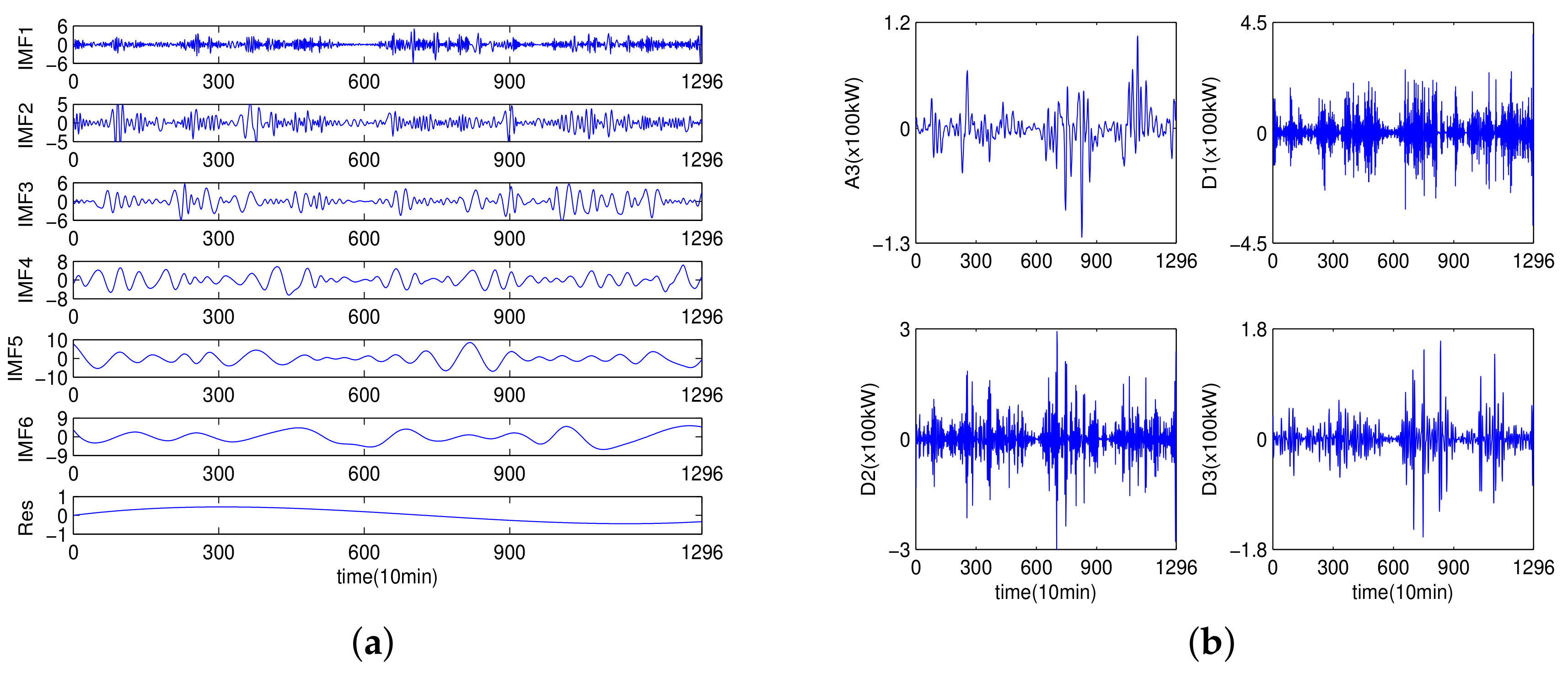
As suggested by Jiang et al. [41], the ensemble number and the amplitude of the added Gaussian distribution white noise in EEMD are set to 100 and 0.2, respectively. Owing to the high fluctuation and randomness characteristic of wind speed, the EEMD algorithm is employed to break the original wind speed data into different relatively stable IMFs and one residual (Res), which is shown in Figure 7a. From IMF1 to Res, the frequencies decrease while the wavelength increases. Among these subseries, IMF1 with highest frequency reveals the detailed information, and the Res reflects the general tendency of original empirical wind speed. In the second decomposition stage, the IMF1 is decomposed into four subseries, namely A3, D1, D2 and D3, by WT to further reduce nonstationarity and fluctuation of IMF1, which is displayed in the Figure 7b.

The input–output candidate matrix of each decomposed subseries is constructed for training and testing. The input vector of each base forecasting engine can be represented as $X_j=f_j(t+1),f_j(t+2),\cdots ,f_j(t+d)$ and the output as $y_j=f_j(t+d+k)$, where $t,d$, and k denote the time point, dimension of input variables, and forecasting step, respectively. Prior to forecasting, the dimensions of the input variables are obtained by the PACF technique. Lags from 1 to 30 are calculated and the input candidate dimensions of the other subseries are listed in

Table 2. Lag values partial autocorrelation function (PACF) for the different subseries.

Data Set	A3	D1	D2	D3	IMF2	IMF3	IMF4	IMF5	IMF6	Res
A	8	7	6	7	12	6	7	6	6	4
B	10	6	8	6	8	9	6	9	8	6

. The input and output format for LSSVM model are displayed as Figure 8, which illustrates that the inputs of the forecasting engine can be from the past values of the target variable.

5.4. Modeling Parameter Selection

The artificial intelligent methods ELM, WNN, and LSSVM and statistical approach ARIMA are employed as the base forecasting engines in the proposed model. The parameters in the artificial intelligent methods are tuned by the optimization algorithm BSA. In the modeling, the parameters are selected as following.

i:

In the ARIMA, the order of autoregressive and moving average play a significant role in the construction of the model and influence its performance. The fitting effects are measured by Akaike’s information criteria (AIC) to determine the lag order of ARIMA; in other words, the smallest AIC values mean the optimal lag order of ARIMA. The detailed parameter selection for ARIMA can be referred to the work by the authors of [37].

ii:

For the BSA algorithm, the population size and iteration number are set as 30 and 100, respectively. The dimension numbers of input nodes, hidden nodes, and output nodes in ELM are set according to the works by the authors of [2,34], and the parameters in WNN are determined according to the work by the authors of [32]. The dimension in BSA-LSSSVM is set as 2.

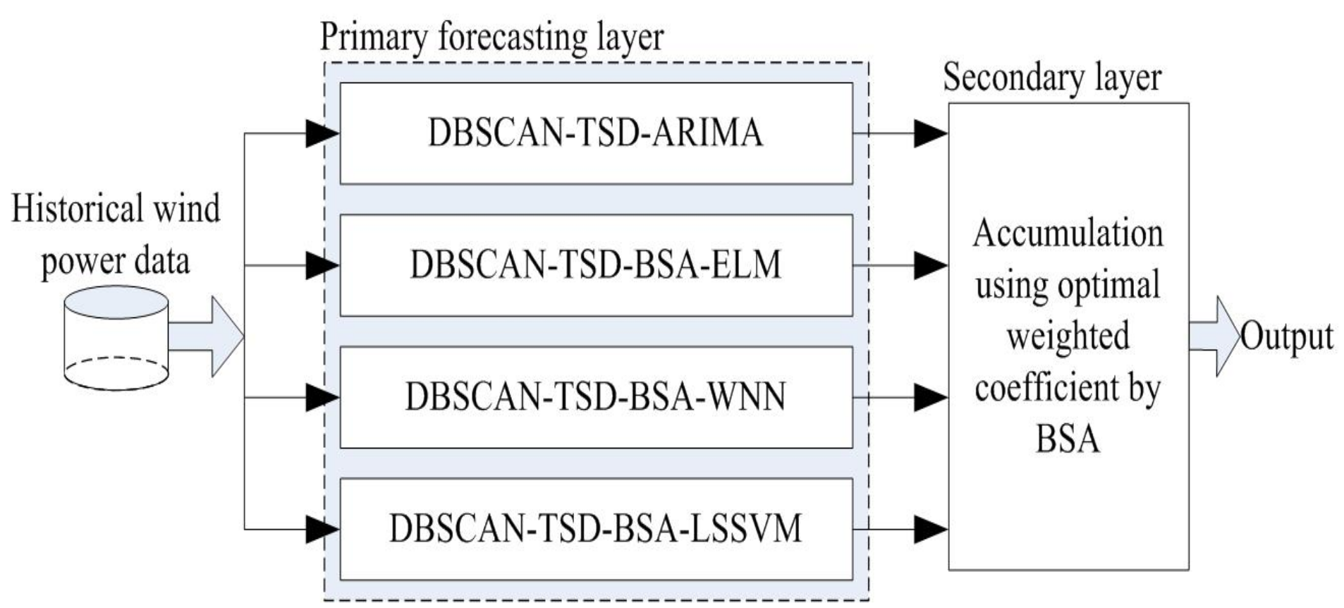
6. Comparisons and Performance Analysis

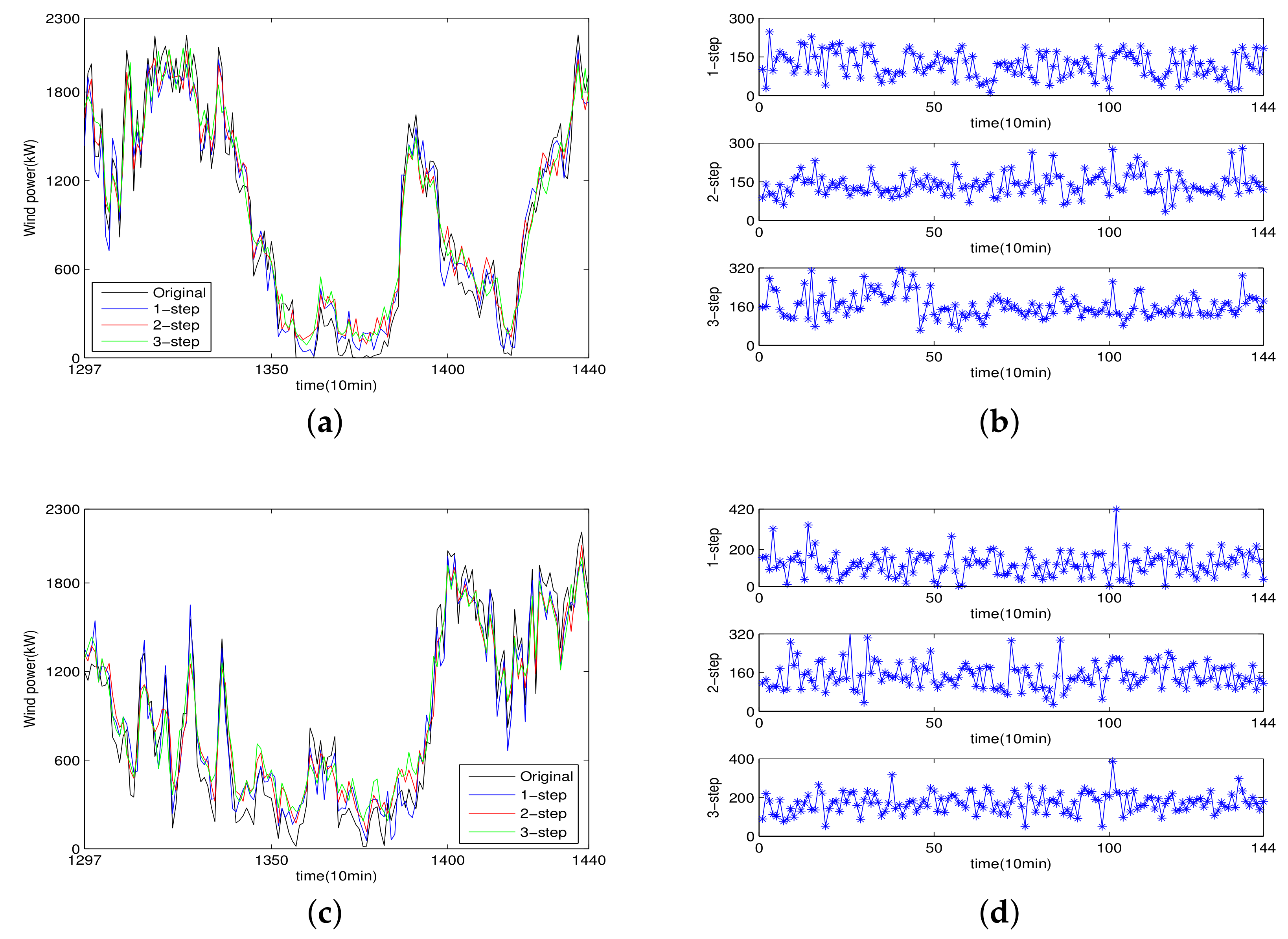
In the proposed WPF, the individual artificial intelligent forecasting engines in the proposed hybrid models are trained and tested using the optimization algorithm with the preprocessed wind power data, and the future 1-day wind power data are predicted in 1-step, 2-step, and 3-step horizontal in the primary forecasting layer. Then, the optimization algorithm BSA is also utilized to make an ensemble of the predicted outputs of the individual forecasting engines by optimal weights in the secondary forecasting layer, and the forecasting results are shown in Figure 9.

To compare and analyze the proposal comprehensively, two categories of experiments are constructed in this section: (1) First, the individual models, including ARIMA, BSA-ELM, BSA-WNN, and BSA-LSSVM, and the individual models with the TSD method, namely, TSD-ARIMA, TSD-BSA-ELM, TSD-BSA-WNN, and TSD-BSA-LSSVM, are established to make multistep WPF; (2) second, four based forecasting models, including DSCAN-TSD-ARIMA, DSCAN-TSD-BSA-ELM, DSCAN-TSD-BSA-WNN, and DSCAN-TSD-BSA-LSSVM, and three recently developed forecasting models are constructed for further comparisons, which can effectively illustrate the superiority of the proposal.

Experiment I: The statistical indexes of the multistep forecasting results and their improved indexes are listed in

Table 3. Forecasting results obtained by different individual models (%).

Data Set	Models	1-Step			2-Step			3-Step
		NMAE	NRMSE		NMAE	NRMSE		NMAE	NRMSE
A	ARIMA	11.4552	12.7560		13.5724	14.3098		14.948	16.1302
	BSA-WNN	9.5132	10.8760		11.3219	12.1886		12.7042	13.4546
	BSA-ELM	9.3438	10.5605		10.5882	11.6710		12.0525	12.9604
	BSA-LSSVM	8.5835	9.8063		9.9734	11.0931		11.7808	12.4766
	TSD-ARIMA	8.8375	9.6144		9.9153	10.5903		11.3281	12.0057
	TSD-BSA-WNN	7.1002	8.0323		8.3087	9.1712		9.4961	10.2937
	TSD-BSA-ELM	6.9839	7.9755		8.0655	9.0816		9.4608	10.3241
	TSD-BSA-LSSVM	6.4898	7.4604		7.9686	8.6205		9.0078	9.6605
	the proposal	5.2666	5.7101		6.5405	6.9165		7.9519	8.3074
B	ARIMA	14.1615	15.2955		14.3199	16.4747		15.9409	17.9055
	BSA-WNN	9.1196	12.3092		10.7669	13.4590		12.5276	14.7803
	BSA-ELM	9.5805	12.3503		10.9315	13.5029		12.4378	14.6774
	BSA-LSSVM	8.6852	11.8929		10.6203	13.0649		13.2596	14.4198
	TSD-ARIMA	9.6087	10.5808		10.2031	11.6028		12.0384	13.0031
	TSD-BSA-WNN	7.4451	8.8870		8.7559	9.8618		9.9223	11.0996
	TSD-BSA-ELM	7.4638	8.4263		8.8018	9.5989		9.6256	10.7062
	TSD-BSA-LSSVM	6.7509	7.7327		8.4016	9.0933		9.2788	10.1088
	the proposal	5.6610	6.3589		7.1099	7.4632		8.3761	8.6682

and

Table 4. The improved normalized mean absolute error (NMAE) and normalized root-mean-square-error (NRMSE) $P_{NMAE}$ and $P_{NRMSE}$ of different forecasting models compared with the proposed model (%).

Data Set	Models	1-Step			2-Step			3-Step
		${\mathit{P}}_{\mathit{NMAE}}$	${\mathit{P}}_{\mathit{RMSE}}$		${\mathit{P}}_{\mathit{NMAE}}$	${\mathit{P}}_{\mathit{RMSE}}$		${\mathit{P}}_{\mathit{NMAE}}$	${\mathit{P}}_{\mathit{RMSE}}$
A	ARIMA	54.0242	55.2363		51.8104	51.666		46.8027	48.4979
	BSA-WNN	44.6389	47.4985		42.2314	43.2548		37.4068	38.2557
	BSA-ELM	43.6349	45.9299		38.2287	40.7382		34.0224	35.902
	BSA-LSSVM	38.6426	41.7711		34.4207	37.6509		32.5010	33.4165
	TSD-ARIMA	40.4056	40.6093		34.0364	34.6905		29.8036	30.8045
	TSD-BSA-WNN	25.8236	28.9108		21.2817	24.5851		16.2602	19.2962
	TSD-BSA-ELM	24.5891	28.4050		18.9080	23.8410		15.9482	19.5342
	TSD-BSA-LSSVM	18.8472	23.4616		16.3173	17.8418		11.7216	14.0065
B	ARIMA	60.0254	58.4261		50.3491	54.6989		47.4551	51.5891
	BSA-WNN	37.9245	48.3399		33.9645	44.5486		33.1383	41.3529
	BSA-ELM	40.9114	48.5116		34.9594	44.7291		32.6559	40.9417
	BSA-LSSVM	34.8198	46.5319		33.0531	42.8760		36.8294	39.8868
	TSD-ARIMA	41.0845	39.9008		30.3157	35.6774		30.4213	33.3377
	TSD-BSA-WNN	23.9628	28.4466		18.7988	24.3218		15.5829	21.9056
	TSD-BSA-ELM	24.1544	24.5348		19.2215	22.2496		12.9804	19.0360
	TSD-BSA-LSSVM	16.1455	17.7655		15.3735	17.9267		9.72819	14.2506

, respectively. As seen from the statistical indices listed in Table 3, some comparisons and analysis for wind power dataset A are carried out as follows.

i:

Among the four individual forecasting models, the BSA-LSSVM approach performs best in multi-step-ahead prediction, the NRMSE values of BSA-LSSVM are smallest. For dataset A, the NRMSE values of BSA-LSSVM are 9.8063%, 11.0931%, and 12.4766% in 1-step, 2-step, and 3-step, respectively, whereas those of BSA-ELM, BSA-WNN, and ARIMA are 10.5605%, 11.6710%, and 12.9604%; 10.8760%, 12.1886%, and 13.4546%; 12.7560%, 14.3098%, and 16.1302% in 1-step, 2-step, and 3-step, respectively. From the statistical indexes, the ARIMA model performs worst in multi-step-ahead prediction.

ii:

From the statistical indexes listed in the Table 3, the four individual forecasting engines with signal decomposition approaches TSD perform better than the four individual forecasting engines without signal decomposition technique. For dataset A, compared with the individual statistical approach ARIMA, the index NRMSE of TSD-ARIMA method leads to reductions of 3.1416%, 3.7195%, and 4.1245% in 1-step, 2-step, and 3-step, respectively; the NRMSE values of TSD-BSA-LSSVM method over those of BSA-LSSVM approach in 1-step, 2-step, and 3-step forecasting are cut by 2.3458%, 2.4726%, and 2.8162%, respectively.

iii:

From the improved indexes listed in the Table 4, the improved index $P_{NRMSE}$ values of the proposal over TSD-ARIMA are 40.6093%, 34.6905%, and 30.8045% for 1-step, 2-step, and 3-step forecasting, respectively. Compared with TSD-BSA-LSSVM, the improved index $P_{NRMSE}$ values of the proposal are 23.4616%, 17.8418%, and 14.0065% for 1-step, 2-step, and 3-step forecasting, respectively.

Remarks: The artificial intelligent models ELM, WNN, and LSSVM have better regression capacity in signal process than statistical approaches ARIMA, especially in dealing with nonlinear signal, because the artificial intelligent models can better capture nonlinear signal components. Not only the statistical model ARIMA, but also the intelligent models WNN, ELM, and LSSVM with signal decomposition TSD, can yield better forecasting performance, the reasons of which are that the original wind powder time series are highly fluctuate, nonlinear, and random and the signal decomposition method TSD decomposes the wind power into a few relatively stable time series and relieves the forecasting difficulties of the four forecasting engines, thus making great contributions to enhance the forecasting performance. For the four based forecasting models, the predicting accuracy decreases with the forecasting step increasing. The LSSVM-based method performs best among the hybrid forecasting models and individual forecasting models because LSSVM excels in dealing with the small sample and nonlinear signals. For the wind power data, B, similar conclusions can be also obtained.

Experiment II: In this section, the forecasting results obtained by four based forecasting models and their improved indexes are listed in the

Table 5. Forecasting results obtained by individual models based on TSD and DBSCAN (%).

Data Set	Models	1-Step			2-Step			3-Step
		NMAE	NRMSE		NMAE	NRMSE		NMAE	NRMSE
A	DBSCAN-TSD-ARIMA	8.3124	8.9385		9.4431	10.1149		10.4781	11.4033
	DBSCAN-TSD-BSA-WNN	6.8698	7.6882		8.0929	8.8733		9.7169	10.3128
	DBSCAN-TSD-BSA-ELM	6.6845	7.4241		7.872	8.6905		9.1861	10.0188
	DBSCAN-TSD-BSA-LSSVM	6.0617	6.9775		7.5309	8.0246		8.8469	9.3999
	the proposal	5.2666	5.7101		6.5405	6.9165		7.9519	8.3074
B	DBSCAN-TSD-ARIMA	8.9655	9.7026		10.3926	11.2242		11.6509	12.7083
	DBSCAN-TSD-BSA-WNN	7.0259	8.2353		8.4681	9.3617		9.4779	10.43019
	DBSCAN-TSD-BSA-ELM	7.2453	7.9738		8.6607	9.2453		9.5571	10.3791
	DBSCAN-TSD-BSA-LSSVM	6.4954	7.3295		8.0224	8.677		8.9815	9.7429
	the proposal	5.6610	6.3589		7.1099	7.4632		8.3761	8.6682

and

Table 6. Improved index $P_{NMAE}$ and $P_{NRMSE}$ of the four based forecasting models compared with the proposed model (%).

Data Set	Models	1-Step			2-Step			3-Step
		${\mathit{P}}_{\mathit{NMAE}}$	${\mathit{P}}_{\mathit{NRMSE}}$		${\mathit{P}}_{\mathit{NMAE}}$	${\mathit{P}}_{\mathit{NRMSE}}$		${\mathit{P}}_{\mathit{NMAE}}$	${\mathit{P}}_{\mathit{NRMSE}}$
A	DBSCAN-TSD-ARIMA	36.6408	36.1181		30.7378	31.8232		24.1093	27.1492
	DBSCAN-TSD-BSA-WNN	23.3362	25.7291		19.1833	22.0534		18.1641	19.4457
	DBSCAN-TSD-BSA-ELM	21.2117	23.0875		16.9145	20.4131		13.4348	17.0819
	DBSCAN-TSD-BSA-LSSVM	13.1161	18.1645		13.1519	13.8093		10.1155	11.6226
B	DBSCAN-TSD-ARIMA	36.8577	34.4614		31.5864	33.5081		28.1073	31.7909
	DBSCAN-TSD-BSA-WNN	19.4267	22.7843		16.0387	20.2799		11.6244	16.8927
	DBSCAN-TSD-BSA-ELM	21.8669	20.2519		17.9059	19.2758		12.35602	16.4841
	DBSCAN-TSD-BSA-LSSVM	12.8459	13.2419		11.3744	13.9893		6.73986	11.0309

, respectively. The proposed WPF integrating the four based forecasting models is employed to make multistep WPF by optimal weighted coefficients. The results show that the integrated forecasting model performs better than the four based benchmark WPF model. From Table 5 and Table 6, the reasons why the proposed compound forecasting strategy can outperform the other hybrid forecasting models are drawn as follows.

i:

As can be seen from Table 3 and Table 5, the four based forecasting engines that are embedded with signal decomposition TSD and abnormal signal identification technique DBSCAN perform better than those based models that embedded with sign decomposition TSD. For dataset A, compared with TSD-ARIMA model, the NRMSE values of DBSCAN-TSD-ARIMA are decreased by 0.6759%, 0.4754%, and 0.6024% in 1-step, 2-step, and 3-step, respectively. Compared with TSD-BSA-LSSVM, the NRMSE values of DBSCAN-TSD-BSA-LSSVM are decreased by 0.4829%, 0.5959%, and 0.3706% in 1-step, 2-step, and 3-step, respectively.

ii:

Each method has its strengths and weaknesses, and every forecasting engine has its own merits and disadvantages. The proposed combined model takes advantages of the individual merits of statistical method and artificial intelligent approaches by optimal weighted coefficients. The model comparisons in terms of statistical indexes illustrate that the proposed combined model outperforms the four based forecasting models. For dataset A in the Table 5, compared with DBSCAN-TSD-ARIMA, the NRMSE values of the proposal lead to reduction of 3.2284%, 3.1984%, and 3.0959%, in 1-step, 2-step, and 3-step, respectively; compared with DBSCAN-TSD-BSA-WNN, the NRMSE values of the proposal lead to reduction of 1.9781%, 1.9567%, and 2.0054% in 1-step, 2-step, and 3-step, respectively; compared with DBSCAN-TSD-BSA-ELM, the NRMSE values of the proposal lead to reduction of 1.714%, 1.7739%, and 1.7114% in 1-step, 2-step, and 3-step, respectively; compared with DBSCAN-TSD-BSA-LSSVM, the NRMSE values of the proposal lead to reduction of 1.2674%, 1.1081%, and 1.0925% in 1-step, 2-step, and 3-step, respectively. Seen from the improved statistical indices in Table 6, compared with the DBSCAN-TSD-BSA-LSSVM model, the $P_{NRMSEs}$ of the proposal are 18.1645%, 13.8093%, and 11.6226% in 1-step, 2-step, and 3-step, respectively. For dataset B, a similar conclusion can be also obtained.

Remark: Compared with the forecasting statistical indexes listed in Table 3 and Table 5, the abnormal data identification DSCAN has improved the prediction accuracy in NRMSE and NMAE values. This is because DBSCAN identifies and discards the abnormal data within the wind power time series and eliminates some disturbing factors. The foregoing operations including abnormal data identification, two-stage decomposition and parameters optimization in the first forecasting layer can make the four based forecasting engines easier to capture and deal with the nonlinear relationship within the wind power time series. The forecasting performance of the individual forecasting engines might change with different wind power time series, which influences seriously the actual industrial application, one solution to this problem is to take advantages of some different plausible forecasting engines.

In the further comparisons, the recently developed models including WPD-HPSOGSA-ELM [34], EEMD-HGSA-LSSVM [39], and TSD-HBSA-DAWNN [42] are constructed to illustrate the effectiveness of the proposed model. The forecasting results and their improved indexes are listed in the

Table 7. Forecasting results obtained by the recently developed models (%).

Data Set	Models	1-Step			2-Step			3-Step
		NMAE	NRMSE		NMAE	NRMSE		NMAE	NRMSE
A	WPD-HPSOGSA-ELM	7.1396	7.7877		8.4412	9.0793		9.7849	10.4674
	TSD-HBSA-DAWNN	6.8182	7.3927		7.9497	8.6379		9.3161	9.9087
	EEMD-HGSA-LSSVM	6.2003	7.0886		7.6483	8.1397		8.9079	9.4313
	the proposal	5.2666	5.7101		6.5405	6.9165		7.9519	8.3074
B	WPD-HPSOGSA-ELM	7.1719	7.9865		9.0313	9.6298		10.219	10.9857
	TSD-HBSA-DAWNN	6.9761	8.1038		8.5585	9.3485		9.7254	10.6243
	EEMD-HGSA-LSSVM	6.5189	7.2795		8.1514	8.7167		9.3243	9.9080
	the proposal	5.6610	6.3589		7.1099	7.4632		8.3761	8.6682

and

Table 8. Improved indexes $P_{NMAE}$ and $P_{NRMSE}$ of the recently developed forecasting models compared with the proposed model (%).

Data Set	Models	1-Step			2-Step			3-Step
		${\mathit{P}}_{\mathit{NMAE}}$	${\mathit{P}}_{\mathit{NRMSE}}$		${\mathit{P}}_{\mathit{NMAE}}$	${\mathit{P}}_{\mathit{NRMSE}}$		${\mathit{P}}_{\mathit{NMAE}}$	${\mathit{P}}_{\mathit{NRMSE}}$
A	WPD-HPSOGSA-ELM	26.2334	26.6781		22.5170	23.8217		18.7326	20.6359
	TSD-HBSA-DAWNN	22.7567	22.7607		17.7268	19.9293		14.6428	16.1607
	EEMD-HGSA-LSSVM	15.0581	19.4469		14.4844	15.0278		10.7315	11.9169
B	WPD-HPSOGSA-ELM	21.0667	20.3788		21.2749	22.4991		18.0359	21.0956
	TSD-HBSA-DAWNN	18.8508	21.5309		16.9253	20.1665		13.8737	18.4116
	EEMD-HGSA-LSSVM	13.1596	12.6462		12.7764	14.3813		9.6009	12.1499

, respectively. As seen from Table 7 and Table 8, the proposed combined forecasting model yields better forecasting performance than the previous developed hybrid models WPD-HPSOGSA-ELM, EEMD-HGSA-LSSVM, and TSD-HBSA-DAWNN for multistep prediction. For example, the improved NRMSEs $P_{NRMSEs}$ of the proposal over the EEMD-HGSA-LSSVM model for dataset A are 19.4469%, 15.0278%, and 11.9169%; for dataset B are 12.6462%, 14.3813% and 12.1499% in 1-step, 2-step, and 3-step, respectively. The way of the proposed wind power prediction model integrating four basic hybrid models by optimal weighted coefficients increases the complexity of the prediction strategy, but it is not a challenging problem for current computer technology.

7. Conclusions

In this study, a compound forecasting strategy combining multiple forecasting enginess with clustering, two-stage decomposition, and parameter optimization is proposed for short-term WPF. The forecasting framework includes four based hybrid forecasting models in the first layer and optimal integration of four individual forecasting models by optimization algorithm BSA in the secondary layer. Two sets of wind power time series are selected from a wind farm located in Anhui, China, to evaluate the performance of the proposed forecasting strategy. From comprehensive comparisons between the proposed model and other different forecasting models, some conclusions can be obtained as follows.

i:

The aforementioned comparisons and analysis illustrate that the prediction performance of the four hybrid models TSD-ARIMA, TSD-BSA-ELM, TSD-BSA-WNN and TSD-BSA-LSSVM can be remarkably improved when compared with the individual forecasting models regardless of BSA-LSSVM, BSA-WNN, BSA-ELM, or ARIMA. Compared with TSD-ARIMA, TSD-BSA-WNN, TSD-BSA-ELM, and TSD-BSA-LSSVM models, these four based forecasting engines with DBSCAN and TSD methods obtain better forecasting results. Therefore, wind power data preprocessing method TSD and DBSCAN can effectively contribute to the forecasting performance of the forecasting engines because TSD decomposes the empirical wind power into relatively reliable components and DBSCAN idenitifies the abnormal wind power data.

ii:

In the primary forecasting layer, the statistical method ARIMA excels in catching the linear variables within wind power, whereas the artificial intelligent approaches ELM, WNN, and LSSVM have good capacities in processing the nonlinear variables. What is more, the artificial intelligent algorithm BSA is employed to optimize the parameters combination in the ELM, WNN, and LSSVM for avoiding local optima. In the end, BSA is developed to tune the weighted coefficients for optimal combination of individual advantages of the four based hybrid forecasting models. Therefore, the proposed hybrid model outperforms all the four based hybrid forecasting models.

iii:

For dataset A, compared with the recently developed forecasting models WPD-HPSOGSA-ELM, TSD-HBSA-DAWNN, and EEMD-HGSA-LSSVM, the NRMSE errors of the proposal are cut by 2.0776%, 2.1628%, and 2.1601%; 1.6826%, 1.7215%, and 1.6013%; and 1.3785%, 1.2232%, and 1.1239% in 1-step, 2-step, and 3-step forecasting, respectively. A similar conclusion can be obtained for dataset B.

Therefore, the proposed hybrid model combining multiple forecasting engines with clustering approach, two-stage decomposition and parameter optimization is an efficient and effective wind power forecasting method. For further studies, this proposed forecasting strategy will be evaluated for other wind farms using environmental and meteorological information and historical wind power data.

References

1. Wang, J.Z.; Heng, J.N.; Xiao, L.Y.; Wang, C. Research and application of a combined model based on multi-objective optimization for multi-step-ahead wind speed forecasting. Energy 2017, 125, 591–613. [Google Scholar] [CrossRef]
2. Abdoos, A.A. A new intelligent method based on combination of VMD and ELM for short term wind power forecasting. Neurocomputing 2016, 203, 111–120. [Google Scholar] [CrossRef]
3. Wang, J.Z.; Hu, J.M. A robust combination approach for short-term wind power forecasting and analysis-Combination of the ARIMA (Autoregressive Integrated Moving Average), ELM (Extreme Learning Machine), SVM (Support Vector Machine) and LSSVM (Least Square SVM) forecasts using a GPR (Gaussian Process Regression) model. Energy 2015, 93, 41–56. [Google Scholar]
4. Jiang, P.; Wang, Y.; Wang, J.Z. Short-term wind speed forecasting using a hybrid model. Energy 2017, 119, 561–577. [Google Scholar] [CrossRef]
5. Brusca, S.; Capizzi, G.; Sciuto, G.L.; Susi, G. A new design methodology to predict wind farm energy production by means of a spiking neural network-based system. Int. J. Numb. Model. 2019, 32, e2267. [Google Scholar] [CrossRef]
6. Meng, A.B.; Ge, J.F.; Yin, H.; Chen, S.Z. Wind speed forecasting based on wavelet packet decomposition and artificial neural networks trained by crisscross optimization algorithm. Energy Convers. Manag. 2016, 114, 75–88. [Google Scholar] [CrossRef]
7. Feng, C.; Cui, M.J.; Hodge, B.M.; Zhang, J. A data-driven multi-model methodology with deep feature selection for short-term wind forecasting. Appl. Energy 2017, 190, 1245–1257. [Google Scholar] [CrossRef] [Green Version]
8. Sun, W.; Wang, Y.W. Short-term wind speed forecasting based on fast ensemble empirical mode decomposition, phase space reconstruction, sample entropy and improved back-propagation neural network. Energy Convers. Manag. 2018, 157, 1–12. [Google Scholar] [CrossRef]
9. Wang, Y.; Hu, Q.H.; Meng, D.Y.; Zhu, P.F. Deterministic and probabilistic wind power forecasting using a variational Bayesian-based adaptive robust multi-kernel regression model. Appl. Energy 2017, 208, 1097–1112. [Google Scholar] [CrossRef]
10. Hoolohan, V.; Tomlin, A.S.; Cockerill, T. Improved near surface wind speed predictions using Gaussian process regression combined with numerical weather predictions and observed meteorological data. Renew. Energy 2018, 126, 1043–1054. [Google Scholar] [CrossRef]
11. Liu, J.Q.; Wang, X.R.; Lu, Y. A novel hybrid methodology for short-term wind power forecasting based on adaptive neuro-fuzzy inference system. Renew. Energy 2017, 103, 620–629. [Google Scholar] [CrossRef]
12. Wang, S.X.; Zhang, N.; Wu, L. Wind speed forecasting based on the hybrid ensemble empirical mode decomposition and GA-BP neural network method. Renew. Energy 2016, 94, 629–636. [Google Scholar] [CrossRef]
13. Liu, H.; Tian, H.; Liang, X. Wind speed forecasting approach using secondary decomposition algorithm and Elman neural networks. Appl. Energy 2015, 157, 183–194. [Google Scholar] [CrossRef]
14. Yin, H.; Dong, Z.; Chen, Y.; Ge, J. An effective secondary decomposition approach for wind power forecasting using extreme learning machine trained by crisscross optimization. Energy Convers. Manag. 2017, 150, 108–121. [Google Scholar] [CrossRef]
15. Peng, T.; Zhou, J.Z.; Zhang, C. Multi-step ahead wind speed forecasting using a hybrid model based on two-stage decomposition technique and AdaBoost-extreme learning machine. Energy Convers. Manag. 2017, 153, 589–602. [Google Scholar] [CrossRef]
16. Liu, T.H.; Wei, H.K.; Zhang, K.J. Wind power prediction with missing data using Gaussian process regression and multiple imputation. Appl. Soft Comput. 2018, 71, 905–916. [Google Scholar] [CrossRef]
17. Zheng, W.Q.; Peng, X.G.; Lu, D.; Zhang, D.; Liu, Y.; Lin, Z.; Lin, L. Composite quantile regression extreme learning machine with feature selection for short-term wind speed forecasting: A new approach. Energy Convers. Manag. 2017, 151, 737–752. [Google Scholar] [CrossRef]
18. Salcedo-Sanz, S.; Pastor-Snchez, A.; Prieto, L. Feature selection in wind power prediction systems based on a hybrid coral reefs optimization-Extreme learning machine approach. Energy Convers. Manag. 2014, 877, 10–18. [Google Scholar] [CrossRef]
19. Niu, X.S.; Wang, J.Y. A combined model based on data preprocessing strategy and multi-objective optimization algorithm for short-term wind speed forecasting. Appl. Energy 2019, 241, 519–539. [Google Scholar] [CrossRef]
20. Zhang, Y.C.; Liu, K.P.; Qin, L. Deterministic and probabilistic interval prediction for short-term wind power generation based on variational mode decomposition and machine learning methods. Energy Convers. Manag. 2016, 112, 208–219. [Google Scholar] [CrossRef]
21. Li, H.M.; Wang, J.Z.; Lu, H.Y.; Guo, Z. Research and application of a combined model based on variable weight for short term wind speed forecasting. Renew. Energy 2018, 116, 669–684. [Google Scholar] [CrossRef]
22. Hou, J.; Gao, H.J.; Li, X.L. DSets-DBSCAN: A parameter-free clustering algorithm. IEEE Trans. Image Process. 2016, 25, 3182–3193. [Google Scholar] [CrossRef] [PubMed]
23. Selim, M.; Emin, A. Improving DBSCAN’s execution time by using a pruning technique on bit vectors. Pattern Recogn. Lett. 2011, 32, 1572–1580. [Google Scholar]
24. Chen, Y.W.; Tang, S.Y.; Bouguila, N. A fast clustering algorithm based on pruning unnecessary distance computations in DBSCAN for high-dimensional data. Pattern Recogn. 2018, 83, 375–387. [Google Scholar] [CrossRef]
25. Galán, S.F. Comparative evaluation of region query strategies for DBSCAN clustering. Inf. Sci. 2019, 502, 76–90. [Google Scholar] [CrossRef]
26. Mahesh Kumar, K.; Rama Mohan Reddy, A. A fast DBSCAN clustering algorithm by accelerating neighbor searching using Groups method. Pattern Recogn. 2016, 58, 39–48. [Google Scholar] [CrossRef]
27. Zhang, C.; Wei, H.K.; Zhao, J.S.; Liu, T.; Zhu, T.; Zhang, K. Short-term wind speed forecasting using empirical mode decomposition and feature selection. Renew. Energy 2016, 96, 727–737. [Google Scholar] [CrossRef]
28. Chitsaz, H.; Amjady, N.; Zareipour, H. Wind power forecast using wavelet neural network trained by improved Clonal selection algorithm. Energy Convers. Manag. 2015, 89, 588–598. [Google Scholar] [CrossRef]
29. Aghajani, A.; Kazemzadeh, R.; Ebrahimi, A. A novel hybrid approach for predicting wind farm power production based on wavelet transform, hybrid neural networks and imperialist competitive algorithm. Energy Convers. Manag. 2016, 121, 232–240. [Google Scholar] [CrossRef]
30. Osorio, G.J.; Matias, J.C.O.; Catalao, J.P.S. Short-term wind power forecasting using adaptive neuro-fuzzy inference system combined with evolutionary particle swarm optimization, wavelet transform and mutual information. Renew. Energy 2015, 75, 301–307. [Google Scholar] [CrossRef]
31. Zhang, C.; Zhou, J.Z.; Li, C.S. A compound structure of ELM based on feature selection and parameter optimization using hybrid backtracking search algorithm for wind power forecasting. Energy Convers. Manag. 2017, 143, 360–376. [Google Scholar] [CrossRef]
32. Sun, S.Z.; Wei, L.S.; Xu, J.; Jin, Z. A new wind power forecasting modeling strategy using two-stage decomposition, feature selection and DAWNN. Energies 2019, 12, 334. [Google Scholar] [CrossRef]
33. Doucoure, B.; Agbossou, K.; Cardenas, A. Time series prediction using artificial wavelet neural network and multi-resolution analysis: Application to wind speed data. Renew. Energy 2016, 92, 202–211. [Google Scholar] [CrossRef]
34. Sun, S.Z.; Fu, J.Q.; Zhu, F. A hybrid structure of an extreme learning machine combined with feature selection, signal decomposition and parameter optimization for short-term wind speed forecasting. Trans. Inst. Meas. Control 2018, 40, 1–18. [Google Scholar] [CrossRef]
35. Yuan, X.H.; Chen, C.; Yuan, Y.B.; Huang, Y.; Tan, Q. Short-term wind power prediction based on LSSVM-GSA model. Energy Convers. Manag. 2015, 101, 393–401. [Google Scholar] [CrossRef]
36. Wu, Q.L.; Peng, C.Y. Wind power grid connected capacity prediction using LSSVM optimized by the bat algorithm. Energies 2015, 8, 14346–14360. [Google Scholar] [CrossRef]
37. Liu, H.; Tian, H.Q.; Li, Y.F. Comparison of two new ARIMA-ANN and ARIMA-Kalman hybrid methods for wind speed prediction. Appl. Energy 2012, 98, 415–424. [Google Scholar] [CrossRef]
38. Civicioglu, P. Backtracking search optimization algorithm for numerical optimization problems. Appl. Math. Comput. 2013, 219, 8121–8144. [Google Scholar] [CrossRef]
39. Su, Z.K.; Wang, H.L.; Yao, P. A hybrid backtracking search optimization algorithm for nonlinear optimal control problems with complex dynamic constraints. Neurocomputing 2016, 186, 182–194. [Google Scholar] [CrossRef]
40. Ahmed, M.S.; Khatib, A.T.; Shareef, H. Real time optimal schedule controller for home energy management system using new binary backtracking search algorithm. Energy Build. 2017, 138, 215–227. [Google Scholar] [CrossRef]
41. Jiang, Y.; Huang, G.Q. Short-term wind power prediction: Hybrid of ensemble empirical mode decomposition, feature selection and error correction. Energy Convers. Manag. 2017, 144, 340–350. [Google Scholar] [CrossRef]
42. Sun, S.Z.; Fu, J.Q.; Zhu, F.; Xiong, N. A compound structure for wind speed forecasting using MKLSSVM with feature selection and parameter optimization. Math. Probl. Eng. 2018, 11, 9287097. [Google Scholar] [CrossRef]
Figure 1. The working flowchart of density-based spatial clustering of applications with noise (DBSCAN).
Energies 12 03586 g001
Figure 2. The working flowchart of ensemble empirical mode decomposition EEMD.
Energies 12 03586 g002
Figure 3. Overall working mechanism of the proposal.
Energies 12 03586 g003
Figure 4. Simplified overall framework of the proposal.
Energies 12 03586 g004
Figure 5. Original wind power time series(kW). (a) Wind power dataset A. (b) Wind power dataset B.
Energies 12 03586 g005
Figure 6. The empirical wind power time series processed by DBSCAN. (a) Abnormal data identified by DBSCAN for set A. (b) Modified wind power by Lagrange interpolation for set A.
Energies 12 03586 g006
Figure 7. Empirical wind power data decomposed by two-stage decomposition (TSD) method. (a) Decomposition of wind power by Ensemble Empirical Mode Decomposition (EEMD) (×100kW). (b) Decomposition of IMF1 by wavelet transform (WT).
Energies 12 03586 g007
Figure 8. Construction of input matrix of the decomposed componoent A 3 of dataset A for the proposed LSSVM.
Energies 12 03586 g008
Figure 9. Forecasting results by the proposed model. (a) Wind power dataset A. (b) Forecasting absolute error for dataset A. (c) Wind power dataset B. (d) Forecasting absolute error for dataset B.
Energies 12 03586 g009