An Asymptotic Numerical Continuation Power Flow to Cope with Non-Smooth Issue

Abstract

Continuation power flow (CPF) calculation is very important for analyzing voltage stability of power system. CPF calculation needs to deal with non-smooth constraints such as the generator buses reactive power limits. It is still a technical challenge to determine the step size while dealing with above non-smooth constraints in CPF calculation. In this paper, an asymptotic numerical method (ANM) based on Fischer-Burmeister (FB) function, is proposed to calculate CPF. We first used complementarity constraints to cope with non-smooth issues and introduced the FB function to formulate the complementarity constraints. Meanwhile, we introduced new variables for substitution to meet the quadratic function requirements of ANM. Compared with the conventional predictor-corrector method combining with heuristic PV-PQ (PV and PQ are used to describe bus types. PV means that the active power and voltage of the bus are known. PQ means that the active and reactive power of bus are known.) bus type switching, ANM can effectively solve the PV-PQ bus type switching problem in CPF calculation. Furthermore, to assure high efficiency, ANM can rapidly approach the voltage collapse point by self-adaptive step size adjustment and constant Jacobian matrix used for power series expansion. However, conventional CPF needs proper step set in advance and calculates Jacobian matrix for each iteration. Numerical tests on a nine-bus network and a 182-bus network validate that the proposed method is more robust than existing methods.

1. Introduction

Power flow calculation is one of the most basic calculation in power system analysis, and it is also the basis of power system stability calculation and fault analysis [1]. Continuation power flow (CPF) calculation combines the continuous method with the static power flow of power system, which is widely used in static voltage stability analysis of power system [2,3,4,5,6,7,8]. However, it is still a technical challenge to deal with the non-smooth constraints such as the reactive power limits violation in CPF calculation [9].

The reactive power limit in CPF calculation has important effects on the voltage stability limit of power system. The traditional method of solving reactive power limit is the logical switch of PV-PQ (PV and PQ are used to describe bus types. PV means that the active power and voltage of the bus are known. PQ means that the active and reactive power of bus are known.) bus type. In [10], a new definition of bus types was presented. The solvability criteria and solution method of bus-type extended power flow are given. And the double switching logic of the new bus types is given to handle the reactive power limits of generators. It is complicated to deal with PV-PQ switch by traditional logic switch method. In [11], a CPF method which considers the reactive limits of generators as a part of the algorithmic procedure was proposed. Lagrange polynomial interpolation formula is used to find the Q-limit breaking point indices. Then the algorithmic continuation steps would be guided by skipping to the closest Q-limit breaking point, consequently reducing the number of continuation steps and saving computational time. With the development of power system research, complementary constraints have been introduced into CPF calculation to deal with the problem of reactive power limit, which greatly improves the solving efficiency.

Reactive power limits can be formulated as complementarity constraints. By using complementary constraints to describe the switching relationship of PV-PQ bus type, the relationship between reactive power and voltage of the bus can be effectively considered without making logical judgment in the process of power flow (PF) iteration. References [12,13] stated that limit-induced constraints on exchange may induce PF divergence. An optimization based model was proposed in [14] to cope with complementarity constraints and was solved using interior point method (IPM). This method is relatively time-consuming since the PF equations are replaced by a constrained optimization problem. To guarantee PF global convergence, in [15,16], trust region based method was proposed to cope with complementarity constraints, whose computation burden even more heavy.

Predictor-corrector method is a conventional CPF calculation method. It involves the prediction of next solution point and correcting the prediction to get the next point on the curve. It includes four parts: prediction, correction, step size control, and parameterization. The values of variables and parameters along the solution curve can be parameterized in a number of ways [17,18].

The contributions of this paper are as follows:

(1)

In this paper, a new CPF calculation method based on asymptotic numerical method (ANM) is proposed, which can only cope with quadratic functions. PV-PQ bus type switch is reformulated by Fischer-Burmeister (FB) functions. FB function is also transformed into quadratic equation to meet the requirements of ANM. Then, ANM is used to calculate the continuous power flow and more robust than predictor-corrector based method to cope with constraints exchange issue. Conventional buses type switch logic methods in CPF, as the number of PV buses changing to PQ increases, the use of logical judgment inevitably increases the burden of calculation, even causing the power flow calculation failed.

(2)

Compared with the conventional predictor-corrector method, ANM can quickly approach the voltage collapse point by self-adaptive step size adjustment and constant Jacobian matrix used for power series expansion, thus greatly improving the CPF calculation efficiency.

2. Establishment and Solution of ANM-CPF

2.1. Semi-Smooth Quadratic Power Flow Equations

The power flow problem is formulated as a set of nonlinear mismatch equations for active and reactive power, as follows,

For a network with $N$ buses, active and reactive power satisfy that:

$$P_i-e_i{\displaystyle \sum _{j=1}^N(G_{ij}{e}_j-B_{ij}{f}_j)-f_i{\displaystyle \sum _{j=1}^N(G_{ij}{f}_j+B_{ij}{e}_j)=0}},$$

(1)

$$Q_i-f_i{\displaystyle \sum _{j=1}^N(G_{ij}{e}_j-B_{ij}{f}_j)+e_i{\displaystyle \sum _{j=1}^N(G_{ij}{f}_j+B_{ij}{e}_j)=0}},$$

(2)

where $P_i$, $Q_i$ are active power and reactive power of bus $i$, $e_i$, $f_i$ are real and imaginary part of bus $i$ voltage, $G_{ij}$, $B_{ij}$ are conductance and susceptance matrix elements respectively.

For PV buses, Equation (2) can be replaced by the equation of voltage:

$${(U_i^{set})}^2-e_i^2-f_i^2=0,$$

(3)

where $U_i^{set}$ is voltage target of PV buses.

For voltage control buses PV and slack bus, when the reactive power exceeds the lower limit, the bus reactive power is set to the lower limit. When the reactive power exceeds the upper limit, the bus reactive power is set to the upper limit. When the bus reactive power does not exceed the limit maintain the original value.

Describe the above relationship with complementary constraints as follows:

$$\{\begin{array}{l}\sqrt{e_i^2+f_i^2}=U_i^{set}+U_i^{+}-U_i^{-},U_i^{+}\ge 0,U_i^{-}\ge 0\\ \left(Q_i-Q_i^{\min }\right)\perp U_i^{+}=0,\forall i\in \left\{PV,Slack\right\}\\ \left(Q_i^{\max }-Q_i\right)\perp U_i^{-}=0,\forall i\in \left\{PV,Slack\right\}\\ Q_i^{\min }\le Q_i\le Q_i^{\max }\end{array},$$

(4)

where $Q_i^{\max }$ and $Q_i^{\min }$ represent the maximum and minimum limits of reactive power of bus $i$ respectively, $U_i^{+}$ and $U_i^{-}$ are slack variables for voltage regulation. There is a general rule of power system. When the reactive power of power system is greater than the maximum limit, the voltage regulation target will be lowered by $-U_i^{-}$, when the reactive power of power system is less than the minimum limit, the voltage regulation target will be enlarged by $+U_i^{+}$.

To cope with the complementarity constraints $u\perp v$, the Fischer-Burmesiter (FB) function [19], is introduced:

$$\varphi \left(u,v\right)=u+v-\sqrt{u^2+v^2+\mu },u\ge 0,v\ge 0,$$

(5)

where a slack variable $\mu ={10}^{-20}$ is introduced to avoid non-differentiable problem of FB at $\left(u=0,v=0\right)$.

In order to turn Equation (5) into a quadratic equation to satisfy the calculation requirements of ANM, we defined a new variable again for variable substitution, the Equation (5) is converted as follows:

$$\varphi \left(u,v\right)=u+v-w,u\ge 0,v\ge 0,w\ge 0,$$

(6)

where $w=\sqrt{u^2+v^2+\mu }$.

FB function has nice properties, such as strong semi-smoothness. Moreover, the squared norm of FB function has a Lipschitz continuous gradient. The FB functions for the complementarity constraints in the power flow can be arranged as:

$$\{\begin{array}{l}{U}_i^{+}+(Q_i-Q_i^{\min })-w_{+}=0\\ {(w_{+})}^2-({(U_i^{+})}^2+{(Q_i-Q_i^{\min })}^2+\mu )=0\\ U_i^{-}+(Q_i^{\max }-Q_i)-w_{-}=0\\ {(w_{-})}^2-({(U_i^{-})}^2+{(Q_i^{\max }-Q_i)}^2+\mu )=0\end{array},$$

(7)

where $w_{+}$ and $w_{-}$ are intermediate variables.

Finally, power mismatch Equations (1)–(3) and (7) constitute the power flow equations, which can be solved by using ANM.

2.2. Algorithm of ANM-CPF

The ANM algorithm is a continuous method for high-order prediction using power series expansion [20]. The solution curve of the nonlinear equation with parameters is segmented, and the solution curve of each segment can be analytically expressed in the form of closed power series. The nonlinear problem is transformed into an infinite amount of linear subproblems, and the sum of the solutions of the first few nonlinear subproblems is used to approximate the real solution. Since the predicted solution is almost the same as the real solution, the ANM-CPF continuous process does not require a correction step in general, and the calculation step size can also be adaptively adjusted.

In order to clearly explain the calculation principle of the ANM algorithm, a two-bus example is introduced in the Appendix A. The detailed calculation process and results are listed there.

Further decompose the above Equations (1)–(3) and Equation (7) by a homotopy transformation:

$$f(x,\lambda )=L(x)+Q(x,x)+\lambda F+H=0,$$

(8)

where $x$ represents variables, including parameters such as the real and imaginary part of bus voltage $e_i$, $f_i$, reactive power $Q_i$, and intermediate variables $w_{+}$ and $w_{-}$. $\lambda$ is the scalar embedding parameter used to describe the increase of active power $P_i$ and reactive power $Q_i$. $L$ and Q represent linear and bilinear operators respectively in Equations (1)–(3) and (7). $F$ is the increase direction of active and reactive power at each bus. $H$ is a constant vector consisting of the reactive power limits $Q_i^{\min }$, $Q_i^{\max }$, slack variable $\mu$, etc. The detailed decomposition process of above power flow equations for the two-bus network corresponds to (A1) and (A4)–(A7) in Appendix A.

Suppose that $(x_t,{\lambda }_t)$ is the $t_{th}(t=0,1,2\dots )$ computed point, the $q_{th}$ point between $t_{th}$ and ${(t+1)}_{th}$ step can be expressed as the series like:

$$\begin{array}{l}{x}_t^q=x_t+{\displaystyle \sum _{p=1}^K{x}_t^{(p)}{(\Delta s)}^q}\\ {\lambda }_t^q={\lambda }_t+{\displaystyle \sum _{p=1}^K{\lambda }_t^{(p)}{(\Delta s)}^q}\end{array},$$

(9)

where $K$ is the truncation order of the series, ${(\Delta s)}^q$ is the step size of $q_{th}$ point between $t_{th}$ and ${(t+1)}_{th}$, $(x_t^{(p)},{\lambda }_t^{(p)})$ is the Taylor coefficients.

The maximum step size is divided into $M$ equal parts. And the step size of $q_{th}$ point between $t_{th}$ and ${(t+1)}_{th}$ satisfies:

$${(\Delta s)}^q=q\frac{\Delta s_{\max }}{M},1\le q\le M,$$

(10)

where $\Delta s_{\max }$ is the maximum step size of the $t_{th}$ computed point and when $q$ is equal to $M$, $x_t^q=x_{t+1}$. The relationship between step size $\Delta s$ and the maximum step size $\Delta s_{\max }$ for a practical two-bus network can be seen in the Table A1 in Appendix A.

The Taylor coefficients $(x_t^{(p)},{\lambda }_t^{(p)})$ at different orders are determined by a series of equations:

Order $p=1$:

$$\begin{array}{l}{f}_x^t{v}_1=-F\\ \left(x_t^{(1)},{\lambda }_t^{(1)}\right)=\pm (v_1,1)/\sqrt{1+{\Vert v_1\Vert }_2^2}\end{array},$$

(11)

Order $p\ge 2$:

$$\begin{array}{l}{f}_x^t{v}_p=-{\displaystyle \sum _{r=1}^{p-1}Q(x_t^{(r)},x_t^{(p-r)})}\\ {\lambda }_t^{(p)}=-{\lambda }_t^{(1)}\langle v_p,x_t^{(1)}\rangle \\ x_t^{(p)}=v_p+{\lambda }_t^{(p)}{v}_1\end{array},$$

(12)

where $f_x^t$ is the value of Jacobian matrix at $x_t$, and $v_1,v_p$ are intermediate variables. Constant Jacobian matrix at $x_t$ is used for each point between $x_t$ and $x_{t+1}$ when using power series expansion. The calculation of Jacobian matrix and Taylor coefficient in a practical two-bus network corresponds to (A8) in Appendix A.

Notice that $Q(x_t^{(r)},x_t^{(p-r)})$ is a matrix composed of functions that construct quadratic terms of the equations:

$$Q(x_t^{(r)},x_t^{(p-r)})=\left[\begin{array}{c}{(x_t^{(r)})}^T*A_Q^1*(x_t^{(p-r)})\\ ⋮\\ {(x_t^{(r)})}^T*A_Q^n*(x_t^{(p-r)})\end{array}\right],$$

(13)

where $A_Q^h(1\le h\le n)$ is a sparse coefficient matrix, the value of $n$ is equal to the dimension of variable $x$.

The maximum step size $\Delta s_{\max }$ satisfies:

$$\Delta s_{\max }={(\epsilon /\Vert ({\displaystyle \sum _{r=1}^{K-1}Q(x_t^{(r)},x_t^{(K-r)})}\Vert )}^{\frac{1}{K}},$$

(14)

where $\epsilon$ is the calculation accuracy control parameter. In view of (A9) and (A10) in Appendix A, the calculation process of the maximum step size $\Delta s_{\max }$ can be seen clearly.

Given (12) and (14), $\Delta s_{\max }$ can be rewritten as follows:

$$\Delta s_{\max }={(\epsilon /\Vert (-f_x^t{v}_K)\Vert )}^{\frac{1}{K}}.$$

(15)

3. Case Study

In this section, case studies are conducted on a small IEEE nine-bus network and a large 182-bus network. The detailed data is referred to [21,22]. The comparison between the ANM and the conventional predictor-corrector method is as follows. Both methods start from the same initial points.

3.1. Example 1: IEEE Nine-Bus Network

3.1.1. Without the Consideration of Reactive Power Limit in CPF

In order to verify the correctness of the ANM, we set the limit of the system reactive power constraint to infinity. This ensures the PV buses or slack bus do not violate the limit in CPF, so the reactive power constraints do not work, as shown in Figure 1. When the scalar embedding parameter $\lambda$ increases to $\lambda =1.641$, the system load power increases to 2.641 times the initial value. The voltage stability limit will be reached, causing the system voltage to collapse.

From Figure 1, we can see that the solutions by using ANM is completely consistent with those by using the conventional predictor-corrector method in PF iteration. It shows that ANM inherits the excellent characteristics of high precision, verifying the correctness of the model and algorithm. In addition, it is easy to conclude that the step size can be adaptively adjusted to improve the calculation speed in PF iteration by using ANM.

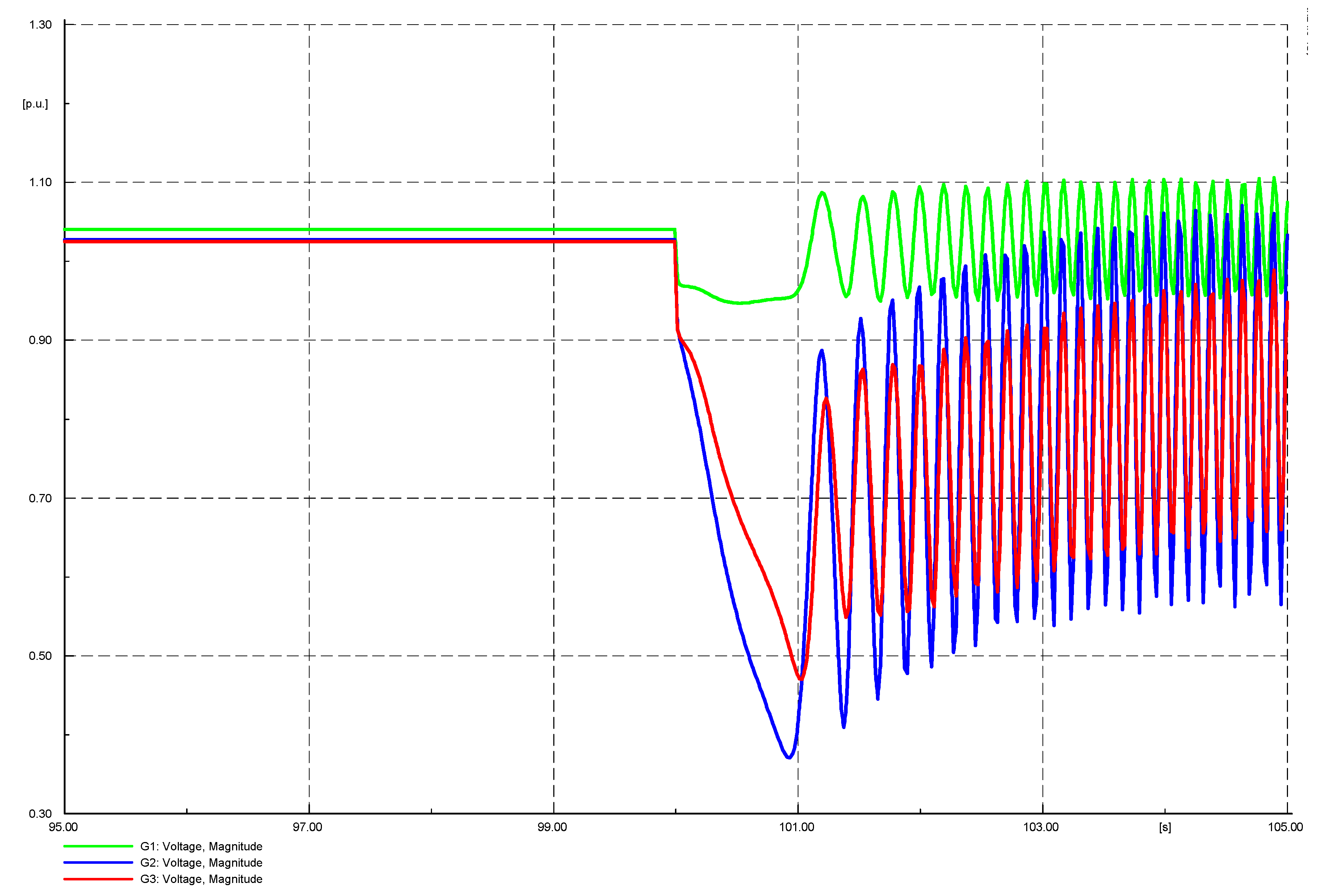
At present, CPF is the most commonly used voltage stability analysis method of large power systems [23,24]. In order to validate the results of the IEEE nine-bus network, we carried out transient stability studies in DlgSILENT. The voltage of slack bus 1, PV buses 2 and 3 remain constant until the scalar embedding parameter $\lambda$ increases to $\lambda =1.641$. When time = 100 s, increase the load power to 2.641 times the initial value, we can see that the voltage of bus 1, 2, and 3 constantly oscillate during the subsequent iterative process, as shown in Figure 2. It proves that the system voltage will be unstable when it reaches the voltage stability limit, which is consistent with the calculation of CPF.

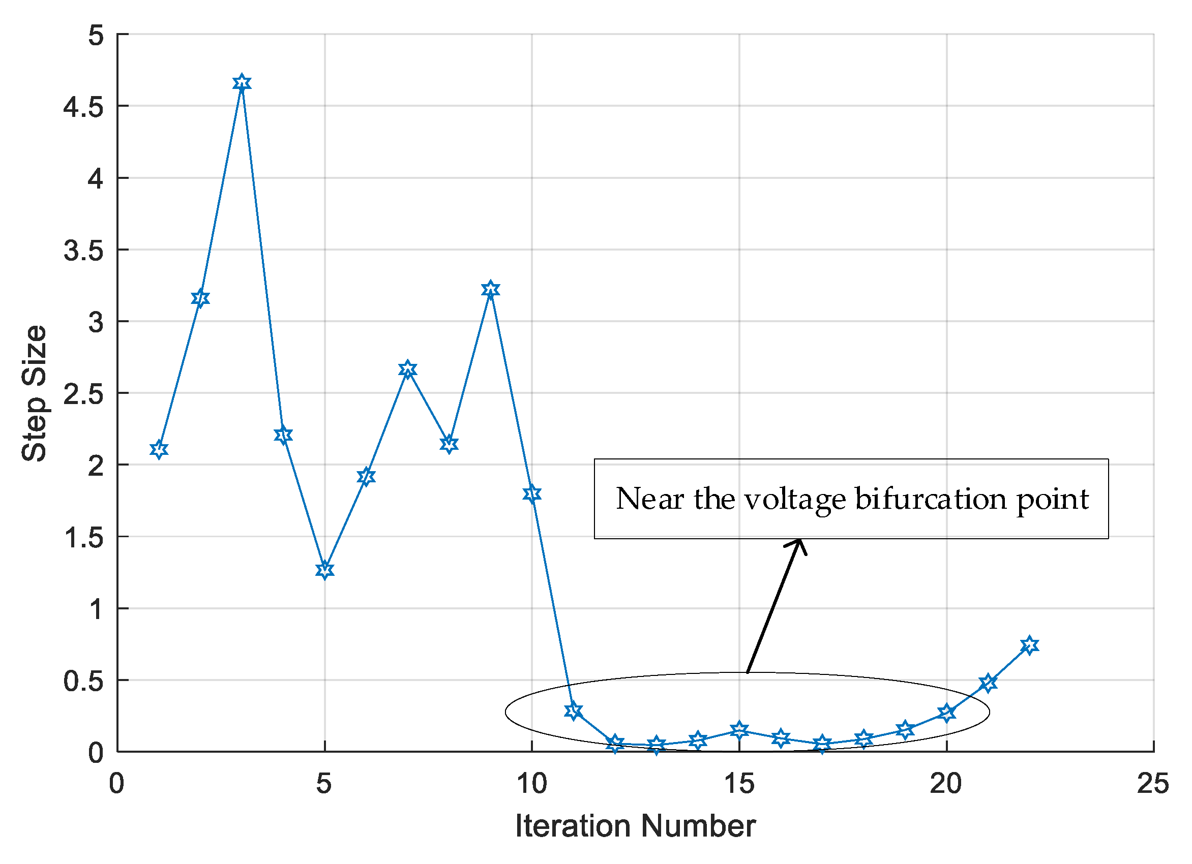
In view of (15), $\Vert (-f_x^t{v}_K)\Vert$ can be understood as the vertical increment of function $f(x,\lambda )$ at point $(x_t,{\lambda }_t)$. When the PV curve gently changes, the vertical increment is small, the maximum step size is large, whereas, when the curve steeply changes, the vertical increment is large, the maximum step size is small. So the step size adaptive adjustment can be realized, as shown in Figure 3. The maximum step size at different points on IEEE nine-bus network can be seen in Figure 4. From Figure 4, we can see that the maximum step size near the voltage bifurcation point is smaller than other points. It can be further verified that the step size of ANM can be adjusted adaptively.

3.1.2. Consideration of Reactive Power Limit in CPF

Considering reactive power limit in CPF, the reactive power limit data of IEEE nine-bus network can be referred to [21]. When scalar embedding parameter $\lambda$ increases to $\lambda =1.533$, the system load power increases to 2.533 times the initial value. The reactive power of bus 1 will violate its reactive power limit, causing the system voltage to collapse, as shown in Figure 5.

The comparison on the central processing unit (CPU) time for both methods is listed in

Table 1. Calculation time of one point in PV curve for both methods.

Method	ANM-CPF	Conventional CPF
Average CPU time for each point/s	$4.01\times {10}^{-4}$	$2.34\times {10}^{-2}$

. In view of Equations (11) and (12), ANM can reduce the time of calculating Taylor coefficient by using constant Jacobian matrix at each point between $x_t$ and $x_{t+1}$ when using power series expansion. The constant Jacobian matrix can lessen calculative burden on the premise of ensuring the accuracy of calculation. However, conventional CPF needs to calculate the Jacobian matrix for each iteration. It can be seen that ANM-CPF using constant Jacobian matrix for power series expansion assure the proposed method more efficient.

When the reactive power of some PV buses and slack bus violate their limits, they are converted to PQ buses or Q$\theta$ (Q$\theta$ is used to describe bus types, which means that the reactive power and phase angle of the bus are known) bus respectively. In the nine-bus system, the conventional predictor-corrector method cannot smoothly realize the PV-PQ bus switching. The step size is $s=0.01$. The PV curves of bus 9 for both methods are as follows. The points of PV curve are sparse near the voltage bifurcation point by using the conventional predictor-corrector method, which is not suitable for obtaining accurate maximum load point. But the ANM can smoothly realize the PV-PQ bus switching and the step size is automatically small near the voltage bifurcation point because of the self-adaptive adjustment. The PV curve can be smoothly drawn, as shown in Figure 6. Correspondingly, no matter how small the step size of conventional predictor-corrector CPF is, the points are still sparse near the voltage bifurcation point, as shown in Figure 7.

3.1.3. Impact of Slack Variable $\mu$ on CPF

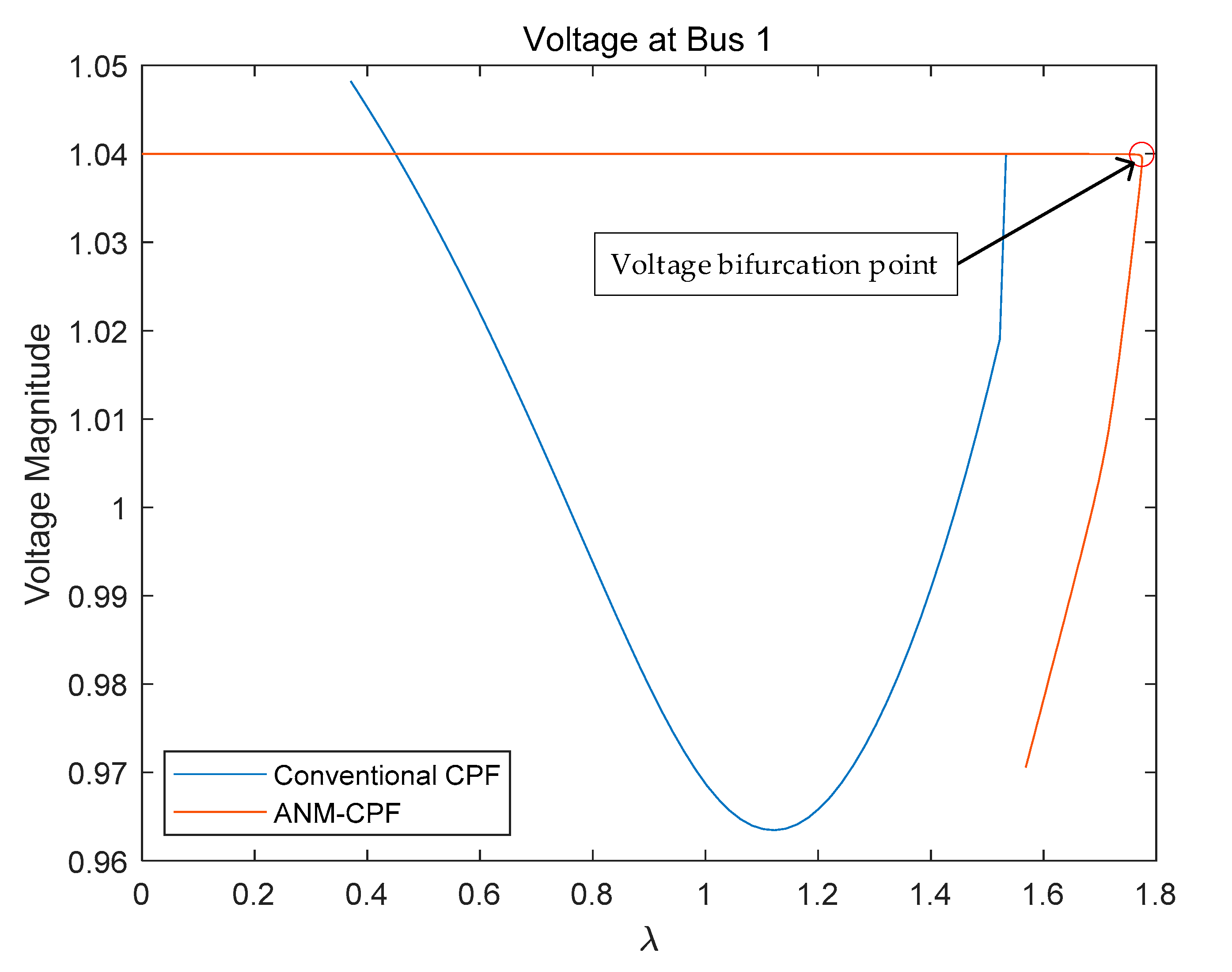
The above calculation results are calculated when the slack variable is $\mu =0$ in Equation (5). In order to further analyze the influence of slack variable value on the calculation result, $\mu ={10}^{-7}$ and $\mu ={10}^{-20}$ are taken successively. We selected the voltage magnitude of bus 1 for both methods to compare. The voltage bifurcation point calculated by ANM is marked in Figure 8 and Figure 9. The comparison results are as follows:

In view of Figure 8 and Figure 9, we can conclude that when the slack variable $\mu$ takes different values, it has different effects on results. The PV curve of conventional CPF is the real solution curve. When $\mu ={10}^{-7}$, ANM will calculate the wrong voltage bifurcation point; when $\mu ={10}^{-20}$, calculated solutions are almost the same as the real solutions. The higher the accuracy of variables for ANM, the less influences on the results. At meanwhile, the calculated solutions are closer to the real solutions.

The comparison on the CPU time for different $\mu$ is listed in

Table 2. Comparison on the central processing unit (CPU) time for different $\mu$.

Slack Variable	$\mathit{\mu }\mathbf{=}{\mathbf{10}}^{\mathbf{-}\mathbf{7}}$	$\mathit{\mu }\mathbf{=}{\mathbf{10}}^{\mathbf{-}\mathbf{20}}$
Average CPU time for each point/s	$3.60\times {10}^{-4}$	$3.52\times {10}^{-4}$

. We can see that when $\mu$ takes different values, there is little difference in CPU time consumed. But ANM still consumes less time and computes more efficiently than conventional predictor-corrector method.

3.2. Example 2: A Large 182-Bus Network

3.2.1. Computation of ANM-CPF

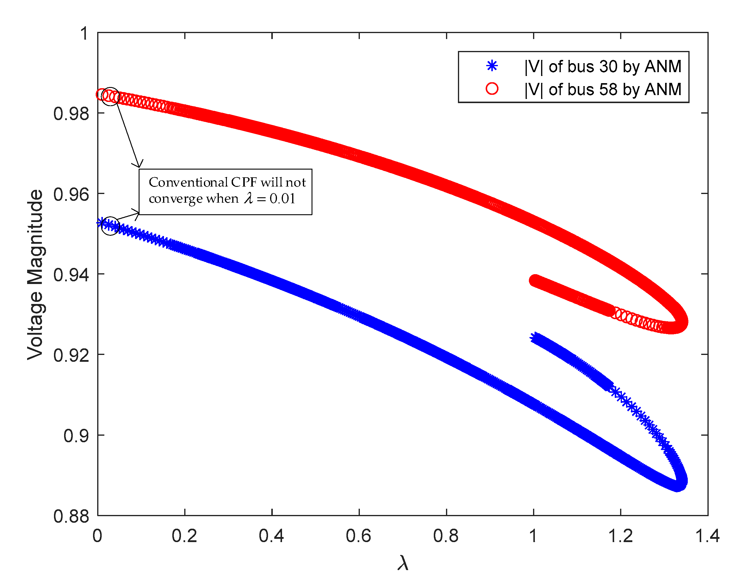
For a 182-bus network, the results of conventional predictor-corrector method are not convergent with the consideration of reactive power limit when the scalar embedding parameter $\lambda$ increases to $\lambda =0.01$. The PV buses or slack bus can be converted to PQ buses or a Q$\theta$ () bus when the reactive power violates their limits by using conventional predictor-corrector method. However, the switch cannot be recovered if the violation temporarily disappears in the sequential iterations. Once the PV buses or slack bus are converted to PQ buses or a Q$\theta$ bus, they cannot be converted back to PV buses or slack bus when the reactive power do not violate the limit, which is not consistent with the actual situation. But ANM can calculate the correct solutions when the scalar embedding parameter $\lambda$ increases to $\lambda =1.340$, the reactive power of bus 70 will violate its reactive power limit causing the system voltage to collapse. We calculated the PV curve of PQ buses, and selected two buses to display, as shown in Figure 10. It further proved that ANM is more robust than conventional predictor-corrector method from the above discussion.

3.2.2. Computation Failures of Conventional CPF

Conventional buses type switch logic methods in CPF, as the number of PV buses changing to PQ increases, the use of logical judgment inevitably increases the burden of calculation, even causing the power flow calculation failing or converging to the wrong solution. When $\lambda =0.01$, from Figure 11, we can see the PV-PQ bus switching strategy leads the conventional predictor-corrector power flow diverging in the large system, and the conventional predictor-corrector method first changed PV buses 59, 65, 103, 19, 34, 92, and 105 to PQ buses at position ①, then converged in five iterations. On sequential iteration, PV buses 49, 55, 56, 61, and 62 changed to PQ buses at position ② and converged in four iterations; PV bus 54 became a PQ bus at position ③; and, finally, PV bus 66 became a PQ bus at position ④. However, due to the number constantly oscillated during the iterative process, the conventional predictor-corrector power flow solution did not converge after 50 iterations from ④. When $\lambda =0.01$, the correct solutions are that PV buses 59, 65, 56, 55, 61, 62, 54, 49, 103, and 66 are changed to PQ buses. Compared to the real solutions, we can see that the conventional predictor-corrector method mistakenly changes the PV buses 19, 34, 92, and 105 to PQ buses because of false logic judgment, which leads to the wrong results during the iteration.

3.2.3. The Reason for the Proposed Method Working

Now let us explain why our proposed method is feasible and effective in the CPF calculation process considering non-smooth constraints exchange issue.

There is a sharp corner at the constraints exchange stage from $Q_i-Q_i^{\min }$ to $U_i^{+}=0$, where the conventional CPF method cannot obtain an accurate direction, which can be mistakenly fixed to PQ buses and cannot go back to PV buses. However, the proposed ANM-CPF based on FB function can solve the problem of the constraints exchange positions at the sharp corner better. It can obtain its local maximum successfully near the sharp point since the direction becomes more smoothly.

4. Conclusions

In this paper, we proposed a CPF calculation method based on the asymptotic numerical method. The algorithm step size can be adaptively adjusted, in addition we introduced a new variable for substitution to meet the calculation requirements of ANM, thus effectively dealing with the problem of reactive power limit. It has certain practicability in solving the problem of CPF in power systems. The small and large power system verify the robustness and efficiency of the proposed method.

References

- Wang, X.-F.; Song, Y.-H.; Irving, M. Modern Power Systems Analysis; Springer: New York, NY, USA, 2008; ISBN 978-0-387-72852-0. [Google Scholar]
- Feng, Z.; Ajjarapu, V.; Long, B. Identification of voltage collapse through direct equilibrium tracing. IEEE Trans. Power Syst. 2000, 15, 342–349. [Google Scholar] [CrossRef]
- Fnaiech, N.; Jendoubi, A.; Zoghlami, M.; Bacha, F. Continuation power flow of voltage stability limits and a three dimensional visualization approach. In Proceedings of the 2015 16th International Conference on Sciences and Techniques of Automatic Control and Computer Engineering (STA), Monastir, Tunisia, 21–23 December 2015; pp. 163–168. [Google Scholar]
- Kumar, S.; Kumar, A.; Sharma, N.K. Analysis of power flow, continuous power flow and transient stability of IEEE-14 bus integrated wind farm using PSAT. In Proceedings of the 2015 International Conference on Energy Economics and Environment (ICEEE), Greater Noida, India, 27–28 March 2015; pp. 1–6. [Google Scholar]
- Garcia, P.A.N.; Vinagre, M.P.; Oliveira, E.J. Fault analysis using continuation power flow and phase coordinates. In Proceedings of the IEEE Power Engineering Society General Meeting, Denver, CO, USA, 6–10 June 2004; Volume 2, pp. 872–874. [Google Scholar]
- Wang, M.; Xia, Y.; Chen, Y.; Huang, S. GPU-based power flow analysis with continuous Newton’s method. In Proceedings of the 2017 IEEE Conference on Energy Internet and Energy System Integration (EI2), Beijing, China, 26–28 November 2017; pp. 1–5. [Google Scholar]
- Cao, B.; Bo, M.; Pan, J.; Liu, Y. Static Voltage Stability Analysis Based on the Combination of Dynamic Continuous Power Flow and Adaptive Chaotic Particle Swarm Optimization. In Proceedings of the 2018 IEEE 3rd Advanced Information Technology, Electronic and Automation Control Conference (IAEAC), Chongqing, China, 12–14 October 2018; pp. 2217–2221. [Google Scholar]
- Canizares, C.A.; Alvarado, F.L. Point of collapse and continuation methods for large AC/DC systems. IEEE Trans. Power Syst. 1993, 8, 1–8. [Google Scholar] [CrossRef]
- Zhao, J.; Zhang, B. Reasons and countermeasures for computation failures of continuation power flow. In Proceedings of the 2006 IEEE Power Engineering Society General Meeting, Montreal, QC, Canada, 18–22 June 2006; p. 6. [Google Scholar]
- Zhao, J.; Zhou, C.; Chen, G. A novel bus-type extended Continuation Power Flow considering remote voltage control. In Proceedings of the 2013 IEEE Power & Energy Society General Meeting, Vancouver, BC, Canada, 21–25 July 2013; pp. 1–5. [Google Scholar]
- Zhu, P.; Taylor, G.; Irving, M. A novel Q-Limit guided Continuation Power Flow method. In Proceedings of the 2008 IEEE Power and Energy Society General Meeting—Conversion and Delivery of Electrical Energy in the 21st Century, Pittsburgh, PA, USA, 20–24 July 2008; pp. 1–7. [Google Scholar]
- Yue, X.; Venkatasubramanian, V.M. Complementary limit induced bifurcation theorem and analysis of Q limits in power-flow studies. In Proceedings of the 2007 iREP Symposium—Bulk Power System Dynamics and Control—VII. Revitalizing Operational Reliability, Charleston, SC, USA, 19–24 August 2007; pp. 1–8. [Google Scholar]
- Avalos, R.J.; Canizares, C.A.; Milano, F.; Conejo, A.J. Equivalency of Continuation and Optimization Methods to Determine Saddle-Node and Limit-Induced Bifurcations in Power Systems. IEEE Trans. Circuits Syst. I Regul. Pap. 2009, 56, 210–223. [Google Scholar] [CrossRef]
- Pirnia, M.; Cañizares, C.A.; Bhattacharya, K. Revisiting the power flow problem based on a mixed complementarity formulation approach. IET Gener. Transm. Distrib. 2013, 7, 1194–1201. [Google Scholar] [CrossRef]
- De Rubira, T.T.; Wigington, A. Extending complementarity-based approach for handling voltage band regulation in power flow. In Proceedings of the 2016 Power Systems Computation Conference (PSCC), Genoa, Italy, 20–24 June 2016; pp. 1–6. [Google Scholar]
- Lin, Y.; Ju, Y. A Robust Three-Phase Power Flow for Active Distribution Network Embedded Autonomous Voltage Regulating Strategies. In Proceedings of the 2018 2nd IEEE Conference on Energy Internet and Energy System Integration (EI2), Beijing, China, 20–22 October 2018; pp. 1–8. [Google Scholar]
- Chiang, H.-D.; Flueck, A.J.; Shah, K.S.; Balu, N. CPFLOW: A practical tool for tracing power system steady-state stationary behavior due to load and generation variations. IEEE Trans. Power Syst. 1995, 10, 623–634. [Google Scholar] [CrossRef]
- Li, S.-H.; Chiang, H.-D. Nonlinear predictors and hybrid corrector for fast continuation power flow. IET Gener. Transm. Distrib. 2008, 2, 341. [Google Scholar] [CrossRef]
- Fischer, A. A special newton-type optimization method. Optimization 1992, 24, 269–284. [Google Scholar] [CrossRef]
- Yang, X.; Zhou, X. Application of asymptotic numerical method with homotopy techniques to power flow problems. Int. J. Electr. Power Energy Syst. 2014, 57, 375–383. [Google Scholar] [CrossRef]
- Zimmerman, R.D.; Murillo-Sanchez, C.E.; Thomas, R.J. MATPOWER: Steady-State Operations, Planning, and Analysis Tools for Power Systems Research and Education. IEEE Trans. Power Syst. 2011, 26, 12–19. [Google Scholar] [CrossRef]
- Ju, Y. Constraints Exchange Data. Available online: https://gitee.com/cieeyodaju/Constraints-Exchange-Data (accessed on 6 August 2019).
- Ruan, C.; Wang, X.; Wang, X.; Gao, F.; Li, Y. Improved Continuation Power Flow Calculation Method Based on Coordinated Combination of Parameterization. In Proceedings of the 2018 IEEE 2nd International Electrical and Energy Conference (CIEEC), Beijing, China, 4–6 November 2018; pp. 207–211. [Google Scholar]
- Alam, M.M.; Moreira, C.; Islam, M.R.; Mehedi, I.M. Continuous Power Flow Analysis for Micro-Generation Integration at Low Voltage Grid. In Proceedings of the 2019 International Conference on Electrical, Computer and Communication Engineering (ECCE), Cox’sBazar, Bangladesh, 7–9 February 2019; pp. 1–5. [Google Scholar]
Figure 1.
V-lambda curve of bus 9 for both methods.
Figure 2.
Voltage transient stability analysis results of bus 1, 2, and 3.
Figure 3.
Vertical increment at different points.
Figure 4.
Maximum step size at different points.
Figure 5.
V-lambda curve of bus 1.
Figure 6.
Figure 7.
Step size for conventional predictor-corrector method.
Figure 8.
V-lambda curve of bus 1 when .
Figure 9.
Figure 10.
V-lambda curve of bus 30 and 58.
Figure 11.
Conventional CPF corrector iteration at .