Hour-Ahead Energy Trading Management with Demand Forecasting in Microgrid Considering Power Flow Constraints

Abstract

Multiple small-scale low-voltage distribution networks with distributed generators can be connected in a radial pattern to form a multi-bus medium voltage microgrid. Additionally, each bus has an independent operator that can manage its power supply and demand. Since the microgrid operates in the market-oriented mode, the bus operators aim to maximize their own benefits and expect to protect their privacy. Accordingly, in this paper, a distributed hour-ahead energy trading management is proposed. First, the benefit optimization problem of the microgrid is solved, which is decomposed into the local benefit optimization sub problems of buses. Then, the local sub problems can be solved by the negotiation of operators with their neighbors. Additionally, the reference demand before negotiation is forecasted by the neural network rather than given in advance. Furthermore, the power flow constraints are considered to guarantee the operational stability. Meanwhile, the power loss minimization is considered in the objective function. Finally, the demonstration and simulation cases are given to validate the effectiveness of the proposed hour-ahead energy trading management.

1. Introduction

With resource exhaustion and environment deterioration, more and more renewable energy generation is being incorporated into the power grid [1,2,3]. However, renewable energy generation, such as wind and solar energy, has the inherent characteristics of randomness and intermittence [4,5,6]. The direct integration of distributed renewable energy into the grid will cause the mismatch of power and finally result in instability. This motivates the development of the microgrid. Actually, the microgrid [7,8,9,10] is a small-scale power distribution system, which is composed of distributed power sources and neighbor loads. When compared with the traditional power grid, the microgrid has several advantages. First, the microgrid can be virtually self-sufficient, which will reduce the long-distance transmission loss. Second, these distributed renewable energy generations can be well used and managed in microgrid. However, in the traditional centralized scheduling of power grid, the renewable energies cannot be fully utilized. Thus, the study of microgrid operation is necessary.

In the microgrid, there are operations for different time periods, namely, the real-time, short-term, mid-term, and long-term [11]. Especially, the hour-ahead operation, which belongs to the short-term operation, may affect the unit commitment [12,13], economic dispatch [14], demand side management [15], spinning reserve scheduling [16], and so on. In the microgrid hour-ahead operation, the demand forecasting plays an important role. Actually, there are various demand forecasting approaches [17], including the multiple regression, fuzzy logic, expert systems, artificial neural networks (ANNs), and so on. Among these demand forecasting methods, the ANN [18,19,20] is preferred because of its higher prediction accuracy, shorter processing time, and stronger adaptation. The development of ANN has entailed three stages until now. The ANN now possesses a larger set of data, a more powerful computer, and a more deeply trained network. When compared to some newly artificial intelligent algorithms, the ANN is fundamental, mature, and easy to perform.

The demand forecasted by ANN [18] can be used as the desired demand in hour-ahead scheduling of microgrid. However, on the one hand, with the increasing application of controllable loads, the demand side has the flexibility to adjust the electricity consumption. On the other hand, the microgrid tends to operate in a market-oriented mode. Thus, an energy trading can happen among electricity suppliers and retailers. The final trading electricity will be decided by the suppliers and retailers rather than the supplier monopoly. To design a new energy trading management framework for the microgrid, two challenges need to be tackled: the utility optimization and the market participants’ privacy protection.

The utility optimization of the microgrid has been discussed in lists of publications [21,22,23]. Reference [21] has studied the electricity cost minimization problem for the residential microgrid with distributed energy resources. References [22,23] both have formulated the operation cost minimization schemes in the droop-controlled microgrid. However, the papers mentioned above only consider the supplier cost. In this paper, the operators of buses take the responsibility of purchasing electricity from the upstream supplier and selling electricity to the local users or downstream buses. These operators can be called retailers in microgrid. The profit earned by these retailers is also considered in the microgrid utility optimization.

In the microgrid utility optimization, most papers only consider the active power, and other power flow parameters, such as reactive power, voltage, and current and so on, are ignored; therefore, the schedule results may violate the stable operation conditions of the microgrid. Therefore, power flow constraints play an important role in the scheduling of the microgrid. Meanwhile, if the power flow equations are added as constraints, the power loss can be calculated. Then, besides the cost and profit, the power loss of transmission is also considered in the objective function.

There exist different kinds of approaches to solve optimization problems. Evolutionary algorithms, such as a hybrid evolutionary method combining particle swarm optimization (PSO) and genetic algorithms (GAs) using fuzzy logic [24], Grey Wolf Optimizer-based algorithms [25], island-based Cuckoo search [26], ideal gas optimization algorithm [27], and so on, can be applied to various optimization systems and proved to be successful. Other than evolutionary algorithms, an exact approach can also solve optimization problems. The radial power flow model in [28,29] can be solved using the convex optimization method. Therefore, in this paper, the microgrid energy trading problem with power flow constraints will be proved to be convex. Convex optimization problems are relatively easy to solve. However, the centralized solution method needs a control center to acquire global information of the microgrid, which causes an invasion of market participants’ privacy and obstructs the process of marketization. Therefore, a distributed energy trading management needs to be designed. References [30,31] introduce a distributed optimization method, the predictor corrector proximal multiplier (PCPM) method. Lagrange multipliers are used to decouple the variables in the objective function. Then, the supplier and retailers of the microgrid can solve their local optimization by negotiating only with neighbors. After the optimization, the social utility of the microgrid is maximized by considering the minimization of power loss.

The main contributions of this paper are summarized as follows.

• The ANN method is used to forecast the demand of LV distribution networks. The hourly forecast results participate in the energy trading as the desired reference demand. This ensures that the final trading decision will not deviate too far from the forecasted demand;
• The power loss minimization is added to the objective function. Additionally, the power flow constraints are also added to the optimization problem. Therefore, in the iteration of optimization, the microgrid operation is guaranteed to be within the allowable range;
• The energy trading optimization problem is solved by decomposing it into local benefit optimization sub problems of the supplier and buses. The local sub problems can be solved by negotiation of operators only with their neighbors. The privacy of market participants is protected.

The paper is organized as follows. In Section 2, the microgrid system framework is introduced. Additionally, the power flow, demand forecasting, and optimization problems of the micro-grid are formulated. Section 3 applies the PCPM algorithm to solving the distributed energy trading management. Numerical examples to complement the theoretical analysis are provided in Section 4. Finally, the conclusion is stated in Section 5.

2. Proposed Microgrid System

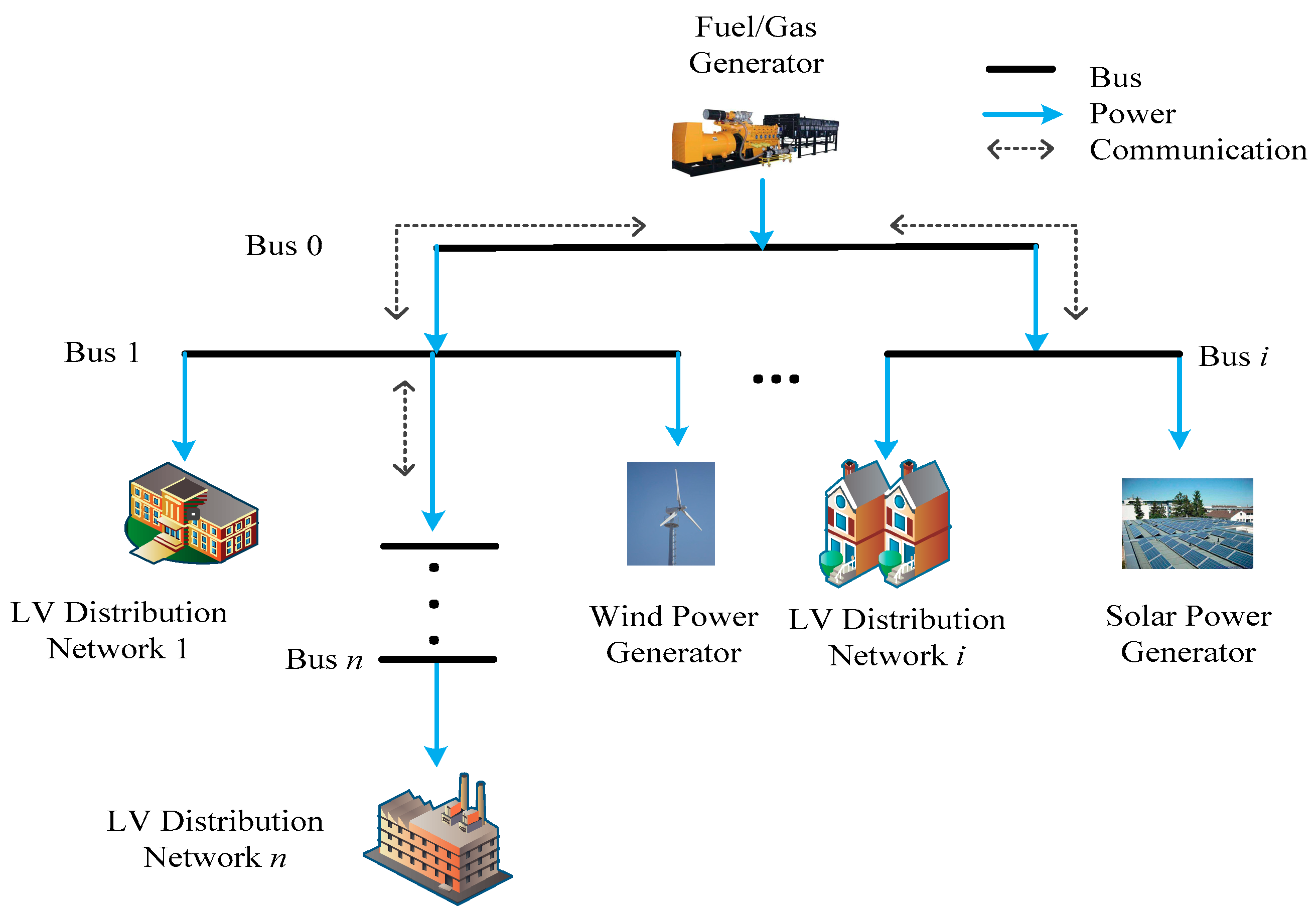
In an islanded electricity supply network, multiple small-scale low voltage (LV) distribution networks can be connected in a radial pattern to form a multi-bus medium voltage microgrid, which is shown in Figure 1. Each bus has an independent operator that can manage its power supply and demand. The operators are equipped with an advanced metering infrastructure that enables bidirectional communication among buses. In this radial microgrid, the fuel/gas generator is the main supplier. The renewable generators, such as wind power generators and solar power generators, can only supply local demand. The operators of buses take the responsibility of purchasing electricity from upstream suppliers and selling electricity to local users or downstream buses. These operators can be called retailers in microgrid.

2.1. Power Flow Constraints

If only active power is considered in the scheduling of the microgrid, and other power flow parameters, such as reactive power, voltage, current, and so on, are ignored, the schedule results may violate the stable operation conditions of the microgrid. Therefore, power flow constraints play an important role in scheduling of the microgrid.

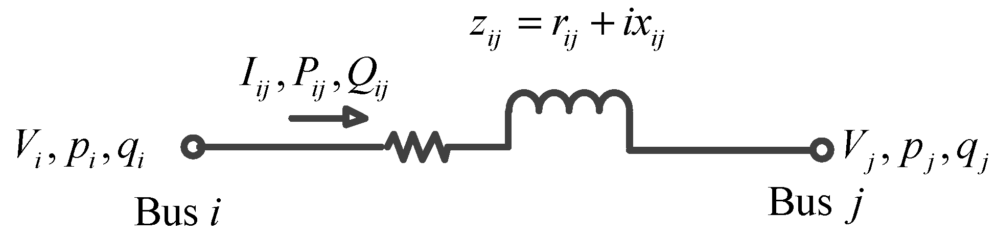
The radial distribution network of the microgrid is modeled as a directed tree graph $T :=\left(N,E\right)$. The buses in set $N$ are indexed by $i=0,1, \dots , n$. Additionally, the distribution line, which connects bus i and bus j, is denoted as $\left(i, j\right)\in E$. The main supplier, the fuel/gas generator, is indexed as bus 0. It is the slack bus, which means its voltage is fixed as $V_0$ and it will supply active and reactive power ($p_0, q_0$) to balance the electricity demand. For each bus $i\in N\backslash \left\{0\right\}$, $V_i$ is its complex voltage and $s_i=p_i+q_i$ is its complex power injection. If the bus has renewable generators, $s_i$ is the demand minus generation. For each line, $\left(i, j\right)\in E$, $I_{ij}$ is the complex current from bus i to bus j. $z_{ij}=r_{ij}+i{x}_{ij}$ is the impedance, and $S_{ij}=P_{ij}+i{Q}_{ij} v$ is the complex power that flows on the distribution line $\left(i, j\right)$. These notations are illustrated in Figure 2.

Given a radial distribution microgrid, the branch flow model [28,29] is as follows:

$$(S_{ij}-z_{ij}{\left|I_{ij}\right|}^2)-{\displaystyle \sum _{k:(j,k)\in E}{S}_{jk}}=s_j,j\in N\backslash \{0\},(i,j)\in E;$$

(1)

$$V_i-V_j=z_{ij}{I}_{ij},(i,j)\in E;$$

(2)

$$S_{ij}=V_i{I}_{ij}^{*},(i,j)\in E.$$

(3)

In order to simplify the notations, $l_{ij}={\left|I_{ij}\right|}^2$, $v_i={\left|V_i\right|}^2$. $V_j=V_i-z_{ij}{S}_{ij}^{*}/V_i^{*}$ can be derived from Equations (2) and (3). If it is squared, then we can get the branch flow model without phase angle of voltage and current

$$p_j=P_{ij}-r_{ij}{l}_{ij}-{\displaystyle \sum _{k:(j,k)\in E}{P}_{jk}},j=1,...,n$$

(4)

$$q_j=Q_{ij}-x_{ij}{l}_{ij}-{\displaystyle \sum _{k:(j,k)\in E}{Q}_{jk}},j=1,...,n$$

(5)

$$v_j=v_i-2(r_{ij}{P}_{ij}+x_{ij}{Q}_{ij})+(r_{ij}^2+x_{ij}^2)l_{ij},(i,j)\in E$$

(6)

$$l_{ij}=\frac{P_{ij}^2+Q_{ij}^2}{v_i},(i,j)\in E.$$

(7)

Reference [28] verifies that if $\left(P, Q, l,v\right)$ is given, the unique phase angle of the radial network can be determined.

2.2. Demand Forecasting Using Artificial Neural Network Method

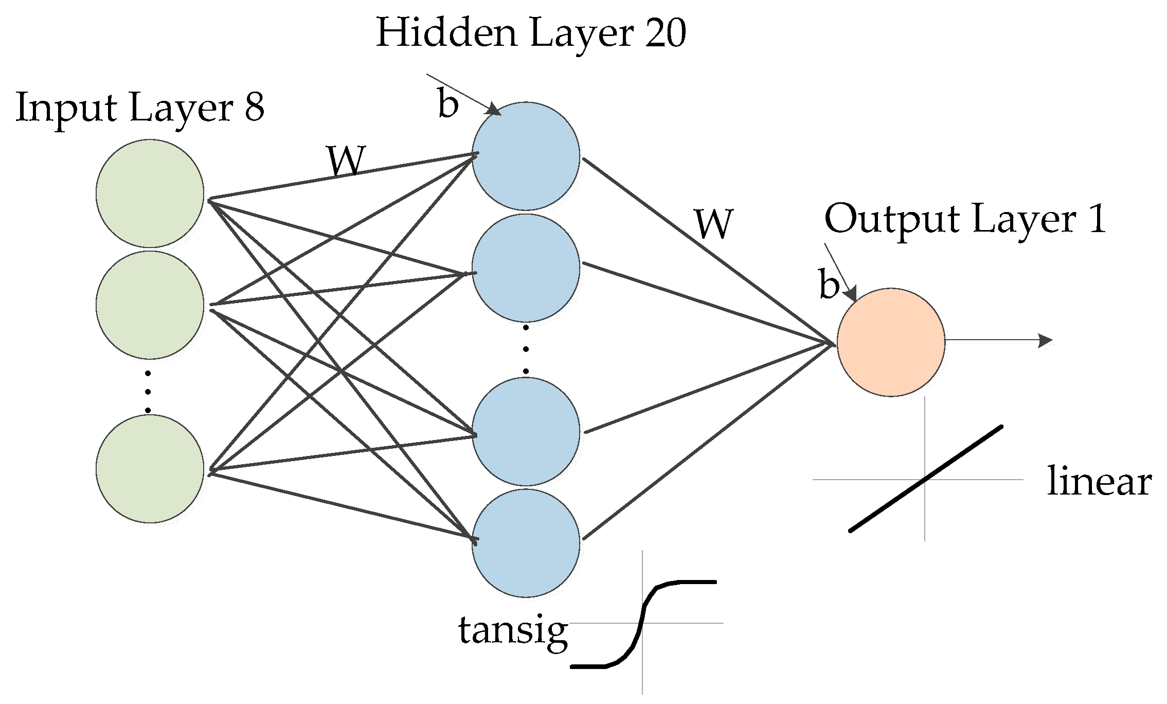
In the energy trading, the accurate forecast of the demand can decrease the waste and maintain stable operation of the power grid. Compared with conventional methods, artificial neural network (ANN) can forecast the demand with higher accuracy. In this paper, the ANN structure is shown in Figure 3. It is a single hidden layer network. In the hidden layer, there are 20 neurons and the activation function is a tansig function. In the output layer, the activation function is a linear function. The training method is Levenberg–Marquardt algorithm. The ANN is trained and tested on a publicly available set of real electricity demand data from the ISO-NE [32]. We extract historical hourly electricity demand data of three zones from 1 January 2016 to 31 December 2018. The hourly weather data of these zones can also be acquired from the ISO-NE. After the preparation of data, the inputs of the training include:

• The dry bulb and dew point temperature;
• The hour and the day;
• The label of holiday/weekend;
• The average demand of previous day;
• The demand from the same hour the previous day;
• The load from the same hour and same day from the previous week.

The data set of years 2016 and 2017 is used to train the ANN. The training set is used for building the model (estimating its parameters). Once the neural network model is built, we can use it to forecast the next hour demand with the eight inputs. The forecasted output result can be compared with the real data from 2018. Then, we can test the performance of the model on out-of-sample data. The performance will be shown in the simulation part. The final hour-ahead forecast output is used as the reference demand of bus i, ${\widehat{p}}_i$.

2.3. Social Utility Maximization

The social utility of the MV microgrid is defined as the profit of LV distribution networks minus the cost of generation. The objective of the microgrid is to maximize the social utility, which is shown in Equation (8). In (8), the power flow constraints are also considered. Therefore, minimization of the power loss of transmission lines can be added to the objective.

$$\begin{array}{l}\max {\displaystyle \sum _{i=1}^n({\lambda }_i{p}_i-\alpha {(p_i-{\widehat{p}}_i)}^2)}-C(p_0)-{\displaystyle \sum _{j\in M}{C}_{jr}}-\rho {\displaystyle \sum _{(i,j)\in E}{r}_{ij}{l}_{ij}}\\ s.t.p_0={\displaystyle \sum _{(0,j)\in E}{P}_{0j}},q_0={\displaystyle \sum _{(0,j)\in E}{Q}_{0j}}\\ p_j=P_{ij}-r_{ij}{l}_{ij}+P_{wj}-{\displaystyle \sum _{k:(j,k)\in E}{P}_{jk}},j\in N\\ q_j=Q_{ij}-x_{ij}{l}_{ij}-{\displaystyle \sum _{k:(j,k)\in E}{Q}_{jk}},j\in N\\ v_j=v_i-2(r_{ij}{P}_{ij}+x_{ij}{Q}_{ij})+(r_{ij}^2+x_{ij}^2)l_{ij},(i,j)\in E\\ l_{ij}=\frac{P_{ij}^2+Q_{ij}^2}{v_i},(i,j)\in E,\\ \underset{\_}{p_i}\le p_i\le \overline{p_i},\underset{\_}{v_i}\le v_i\le \overline{v_i},i=1,\cdots ,n.\end{array}$$

(8)

In the Equation (8), ${\lambda }_i$ is the retail electricity price of bus i. Even if consumers of buses own controllable applications, $\mathsf{\alpha }$ is penalty coefficient of the difference between reference demand ${\widehat{p}}_i$ and final supply $p_i$. The initial reference demand ${\widehat{p}}_i$ can be obtained by the ANN method. $\mathrm{C}\left(p_0\right)$ is the cost function of the fuel/gas generator. It is indicated by a quadratic function [33] $\mathrm{C}\left(p_0\right)=b_1{p}_0^2+b_2{p}_0+b_3$, where $b_1>0, b_2, b_3\ge 0$ are varying fuel/gas coefficients. The parameter $C_{jr}$ is used to represent the fixed hourly cost of renewable generators at bus j. The coefficient $\rho$ can adjust the weight of the power loss term.

The quadratic Equation (7) is a constraint in (8). Because it is non-affine, (8) is not convex. Reference [28] relaxes it into an inequality constraint, which can convex the power flow constraints.

$$l_{ij}\ge \frac{P_{ij}^2+Q_{ij}^2}{v_i},(i,j)\in E.$$

(9)

(9) can be converted to a second-order cone constraint as follows:

$${\Vert \begin{array}{c}(l_{ij}-v_i)/2\\ P_{ij}\\ Q_{ij}\end{array}\Vert }_2\le (l_{ij}+v_i)/2$$

Then, the convex optimization function of microgrid utility maximization is function (8) with substitutional constraint (9).

The validity conditions for the relaxation is proposed in [28]. In the paper, it is easy to satisfy the conditions considering the structure of the microgrid.

After the second-order cone relaxation, the objective function becomes convex, which can be solved centrally. However, a control center is needed to take the responsibility of global control; it requires detailed information of the microgrid, which causes privacy issues. With market-oriented reform, operators of buses aim to maximize their own benefits and expect to protect their privacy during trading. Therefore, the microgrid social utility maximization problem needs to be solved using distributed mechanisms.

3. Distributed Energy Trading Management Scheme

3.1. Introduction of Predictor Corrector Proximal Multiplier Method

Predictor corrector proximal multiplier (PCPM) [30,31] is a method to solve convex minimization problems in the decomposition approach. Considering a convex problem in the generic form

$$\min \{f(x)+g(z):Ax=z\}.$$

The Lagrangian of this problem is

$$L(x,z,y)=f(x)+g(z)+y(Ax-z).$$

where y is the Lagrangian multiplier.

The distributed algorithm can be written as

$$\begin{array}{l}{p}^{k+1}=\arg \max \{L(x^k,z^k,y)-(1/(2{\lambda }_k)){\Vert y-y^k\Vert }^2\},\hfill \\ x^{k+1}=\arg \min \{L(x,z^k,p^{k+1})+(1/(2{\lambda }_k)){\Vert x-x^k\Vert }^2\},\hfill \\ z^{k+1}=\arg \min \{L(x^k,z,p^{k+1})+(1/(2{\lambda }_k)){\Vert z-z^k\Vert }^2\},\hfill \\ y^{k+1}=\arg \max \{L(x^{k+1},z^{k+1},y)-(1/(2{\lambda }_k)){\Vert y-y^k\Vert }^2\}.\hfill \end{array}$$

where ${\mathsf{\lambda }}_k$ is a positive scalar. In this algorithm, $p^{k+1}$ is the predictor step, $y^{k+1}$ is the corrector step, and $x^{k+1}$, $z^{k+1}$ are separable proximal steps. After iterations, the PCPM method will converge to a global optimal solution.

3.2. Distributed Solution Method

The variables in the function (8) with substitutional constraint (9) can be decoupled and computed separately from each other using the PCPM method. Lagrange multipliers ${\mu }_i$ are associated with the active power equation constraints. They can be used to decompose the objective function of microgrid to sub problems that can be solved locally. Lagrange multiplier ${\mu }_i$ can be treated as a price guidance signal. It is not the real electricity price, because of the power loss term in the objective function. The sub problems solved by supplier and buses are defined in the following section.

3.2.1. Solving Supplier Cost Minimization

As a supplier of the microgrid, the supplier sells electricity to its users. According to the cost of generation and the demand of its users, the supplier will design an appropriate price to maximize its own utility. The objective function of the supplier is presented as function (10). ${\widehat{v}}_i$ is the estimation of children node voltages. The coefficient ${\mathsf{\omega }}_i$ is the Lagrange multiplier associated with the voltage estimation. $x^{*}$ is the optimization of the last iteration.

$$\begin{array}{l}\max {\displaystyle \sum _{(0,i)\in E}{\mu }_i(P_{0i}-r_{0i}{l}_{0i})}-C(p_0)-\rho {\displaystyle \sum _{(0,i)\in E}{r}_{0i}{l}_{0i}}+{\displaystyle \sum _{(0,i)\in E}{\omega }_i{\widehat{v}}_i}-\frac{1}{2\gamma }{\Vert x-x^{*}\Vert }_2^2\\ over:x:=(P_{0i},Q_{0i},l_{0i},{\widehat{v}}_i,p_0,q_0)\\ s.t.p_0={\displaystyle \sum _{(0,i)\in E}{P}_{0i}},q_0={\displaystyle \sum _{(0,i)\in E}{Q}_{0i}},\\ Q_{0i}=x_{0i}{l}_{0i}+{\displaystyle \sum _{k:(i,k)\in E}{Q}_{ik}},i\in N\backslash \left\{0\right\}\\ {\widehat{v}}_i=v_0-2(r_{0i}{P}_{0i}+x_{0i}{Q}_{0i})+(r_{0i}^2+x_{0i}^2)l_{0i},(0,i)\in E\\ l_{0i}\ge \frac{P_{0i}^2+Q_{0i}^2}{v_0},(0,i)\in E,\\ \underset{\_}{p_0}\le p_0\le \overline{p_0}.\end{array}$$

(10)

3.2.2. Solving Buses Utility Maximization

Buses except the slack bus will buy electricity from its upstream supplier. If it has child nodes, it will sell electricity to downstream buses. Therefore, buses are separated into two kinds. One is the leaf nodes, which have no child node. The other is the nodes that have child nodes. The utility maximization problems of these two kinds of nodes are as follows:

• Bus $i\in N\backslash \left\{0\right\},$ such that $\left(i, j\right)\in E$, $j\in N\backslash \left\{0\right\}$ solves the following problem:

  $$\begin{array}{l}\max {\lambda }_i{p}_i-{\alpha }_i{(p_i-{\widehat{p}}_i)}^2-{\displaystyle \sum _{i\in M}{C}_{ir}}-{\mu }_i(p_i+{\displaystyle \sum _{(i,j)\in E}{P}_{ij}})+{\displaystyle \sum _{(i,j)\in E}{\mu }_j(P_{ij}-r_{ij}{l}_{ij})}\\ -\rho {\displaystyle \sum _{(i,j)\in E}{r}_{ij}{l}_{ij}}-{\displaystyle \sum _{(k,i)\in E}{\omega }_i{v}_i}+{\displaystyle \sum _{(i,j)\in E}{\omega }_j{\widehat{v}}_j}-\frac{1}{2\gamma }{\Vert y-y^{*}\Vert }_2^2\\ over:y:=(P_{ij},Q_{ij},l_{ij},v_i,{\widehat{v}}_j,p_i)\\ s.t.Q_{ij}=x_{ij}{l}_{ij}+{\displaystyle \sum _{k:(j,k)\in E}{Q}_{jk}},j\in N\\ {\widehat{v}}_j=v_i-2(r_{ij}{P}_{ij}+x_{ij}{Q}_{ij})+(r_{ij}^2+x_{ij}^2)l_{ij},(i,j)\in E\\ l_{ij}\ge \frac{P_{ij}^2+Q_{ij}^2}{v_i},(i,j)\in E,\\ \underset{\_}{p_i}\le p_i\le \overline{p_i},\underset{\_}{v_i}\le v_i\le \overline{v_i},i=1,\cdots ,n.\end{array}$$

  (11)
• Bus $i\in N\backslash \left\{0\right\},$ such that $\left(i, j\right)\notin E$, for all $j\in N\backslash \left\{0\right\}$, solves the following problem:

  $$\begin{array}{l}\max {\lambda }_i{p}_i-{\alpha }_i{(p_i-{\widehat{p}}_i)}^2-{\displaystyle \sum _{i\in M}{C}_{ir}}-{\mu }_i{p}_i-{\displaystyle \sum _{(k,i)\in E}{\omega }_i{v}_i}-\frac{1}{2\gamma }{\Vert z-z^{*}\Vert }_2^2\\ over:z:=(v_i,p_i)\\ s.t.\underset{\_}{p_i}\le p_i\le \overline{p_i},\underset{\_}{v_i}\le v_i\le \overline{v_i},i=1,\cdots ,n.\end{array}$$

  (12)

3.3. Algorithm Design and Implementation

According to the PCPM method, buses will solve their utility maximization locally. The distributed energy trading algorithm is presented in Algorithm 1.

Algorithm 1 Distributed Hour-Ahead Energy Trading

The slack bus 0 chooses initial values for variable set x and Lagrange multipliers ${\lambda }_i$ for its child nodes such that $\left(0,i\right)\in E$. Each bus $i\in N\backslash \left\{0\right\}$ such that $\left(i, j\right)\in E$, $j\in N\backslash \left\{0\right\}$, chooses initial values for variable set y and Lagrange multipliers ${\lambda }_j$ for its child nodes such that $\left(i,j\right)\in E$. Each bus $i\in N\backslash \left\{0\right\}$ such that $\left(i, j\right)\notin E$, for all $j\in N\backslash \left\{0\right\}$, chooses initial values for variable set z. Then, while $k\ge 0$: every node repeat steps 2–6 until convergence. Each bus $j\in N\backslash \left\{0\right\}$ transmits its demand $p_j$ and voltage $v_j$ to its parent node $i\in N$, $\left(i,j\right)\in E$. The parent node i will update the Lagrange multipliers as follows: $$\begin{array}{l}{\widehat{\lambda }}_j^k:={\lambda }_j^k-\gamma \left(P_{ij}^k-{\displaystyle \sum _{(i,j),(j,h)\in E}(P_{jh}^k+r_{ij}{l}_{ij}^k+p_j^k)}\right),\\ {\stackrel{⌢}{\omega }}_j^k:={\omega }_j^k-\gamma \left({\widehat{v}}_j^k-v_j^k\right).\end{array}$$ Each parent node sends the updated Lagrange multipliers to its child nodes. Each node optimize local variables according to (11), (12) and (10) simultaneously. Each bus $j\in N\backslash \left\{0\right\}$ transmits its demand $p_j$ and voltage $v_j$ to its parent node $i\in N$. The parent node i will update the Lagrange multipliers as follows: $$\begin{array}{l}{\widehat{\lambda }}_j^{k+1}:={\lambda }_j^k-\gamma \left(P_{ij}^{k+1}-{\displaystyle \sum _{(i,j),(j,h)\in E}(P_{jh}^{k+1}+r_{ij}{l}_{ij}^{k+1}+p_j^{k+1})}\right),\\ {\stackrel{⌢}{\omega }}_j^{k+1}:={\omega }_j^k-\gamma \left({\widehat{v}}_j^{k+1}-v_j^{k+1}\right).\end{array}$$ $k\leftarrow k+1$, return to step 2.

4. Evaluation

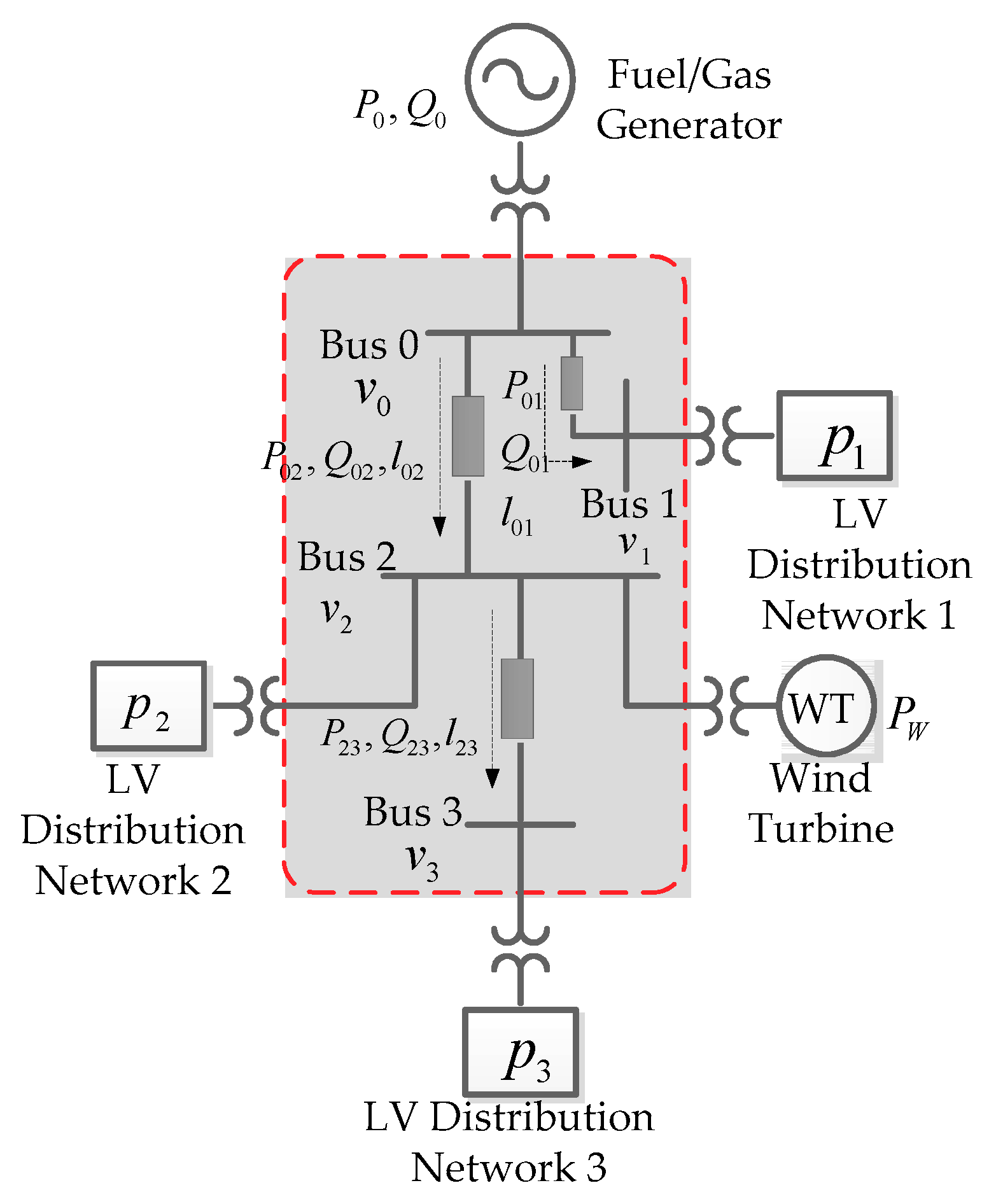
Most of microgrids are carried out by simulation, which is difficult to perform in a real situation. Considering the fact, in this section, numerical examples are provided to complement the analysis. In order to make the demonstration and simulation more reliable, the work is verified by simulation based on the real data. The simulation is implemented to a medium-voltage microgrid distribution network, as shown in Figure 4. There are four buses. Bus 0 is the slack bus that connects to a fuel/gas generator. The voltage of it is 4.16 kV, which refers to the IEEE 13 Node Test Feeder system. The cost function of the generator is $\mathrm{C}\left(p_0\right)=0.8p_0^2+10p_0$. Its generation limit is $p_0\in \left[2MW,7MW\right]$. The other three buses provide electricity to LV distribution networks respectively. And a wind turbine is connected to bus 2. The hourly wind power generation data is retrieved from independent electricity system operator (IESO) [34]. The fixed cost is assumed to be $1 for one hour. The distribution line parameters are listed in

Table 1. Microgrid distribution line parameters.

Distribution Line	Type	Parameters
0–1	1 km JKLYJ-50	0.62 + j 0.30 $\mathsf{\Omega }$
0–2	1.5 km JKLYJ-70	0.69 + j 0.47 $\mathsf{\Omega }$
2–3	1 km JKLYJ-35	0.85 + j 0.26 $\mathsf{\Omega }$

. In order to better explain the detailed process of evaluation, a block diagram is presented in Figure 5.

4.1. Demand Forecasting Results

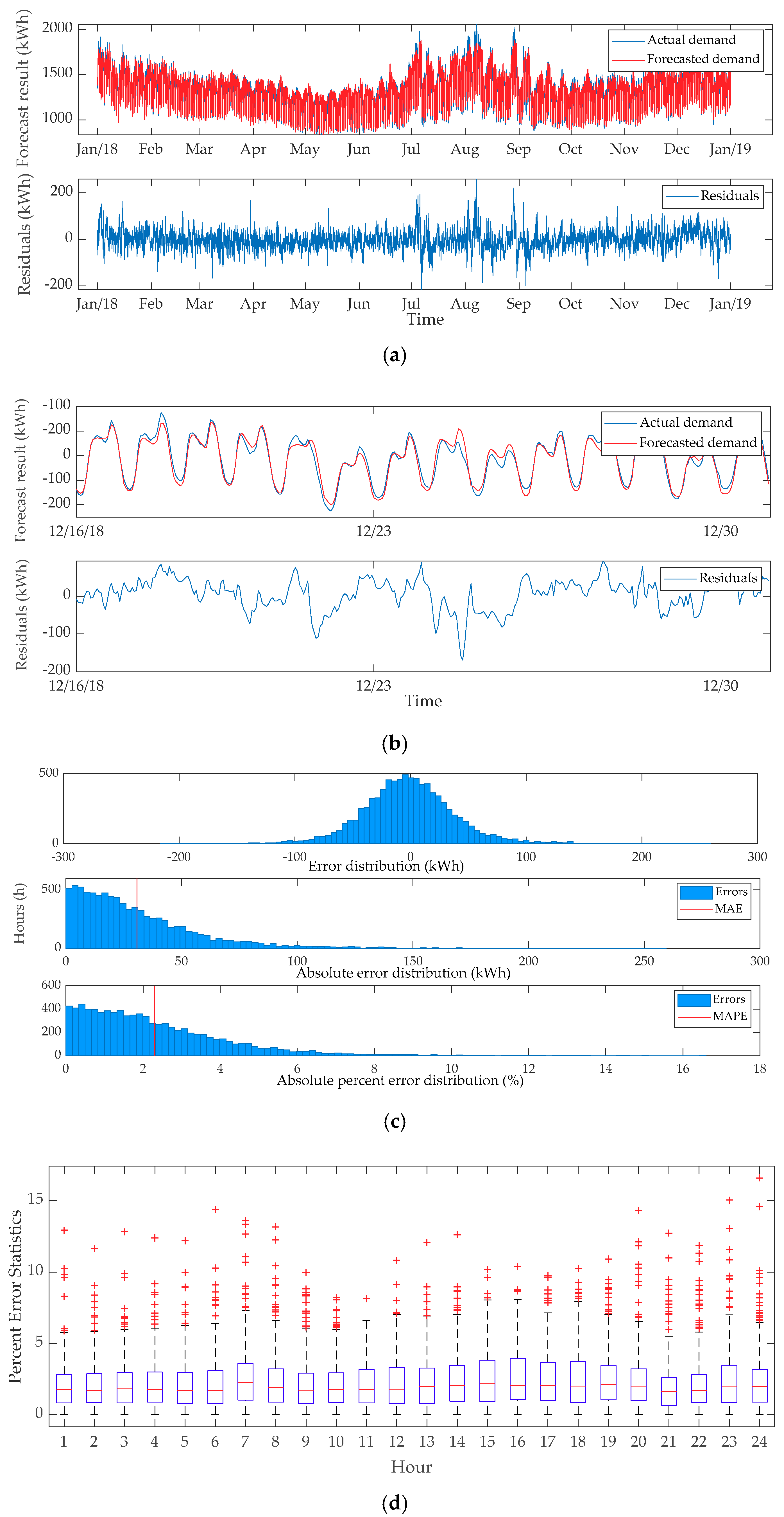
The demands of LV distribution networks announced by operators are forecasted by ANN method using real historical electricity data and weather information. The ANN is trained in MATLAB using the neural network toolbox. Figure 6a,b shows the comparison of the actual demand and the forecasted demand. Figure 6a shows the results from a whole year while Figure 6b shows the results from 2 weeks. The error distribution is presented in Figure 6c,d. The mean absolute error (MAE) is 30.67 kWh, and mean absolute percent error (MAPE) is 2.3%. The hour-ahead forecasted demand ${\widehat{p}}_i$ of 3 LV distribution networks is accurate enough to be used as the reference demand in trading.

4.2. Energy Trading Results

Each LV distribution network uses ANN to forecast its demand ${\widehat{p}}_i$ for the next hour. The original system data with ${\widehat{p}}_i$ is shown in

Table 2. Original bus data.

Bus	Voltage	Generation		Demand
	Mag (pu)	P (MW)	Q (MVAr)	P (MW)	Q (MVAr)
0	1.0000	3.9223	0.1909	-	-
1	0.9374	-	-	1.6285	0
2	0.9106	0.1890	0	1.4535	0
3	0.8712	-	-	0.6983	0

and

Table 3. Original branch data.

Branch	Branch Power		Loss
	P (MW)	Q (MVAr)	P (MW)	Q (MVAr)
0–1	1.7366	0.0522	0.1081	0.0522
0–2	2.1857	0.1387	0.1914	0.1291
2–3	0.7298	0.0096	0.0315	0.0096
		Total:	0.3310	0.1909

. The retail prices of LV distribution networks are 21, 22, and 23, respectively. The power flow information is calculated by the MATPOWER [35].

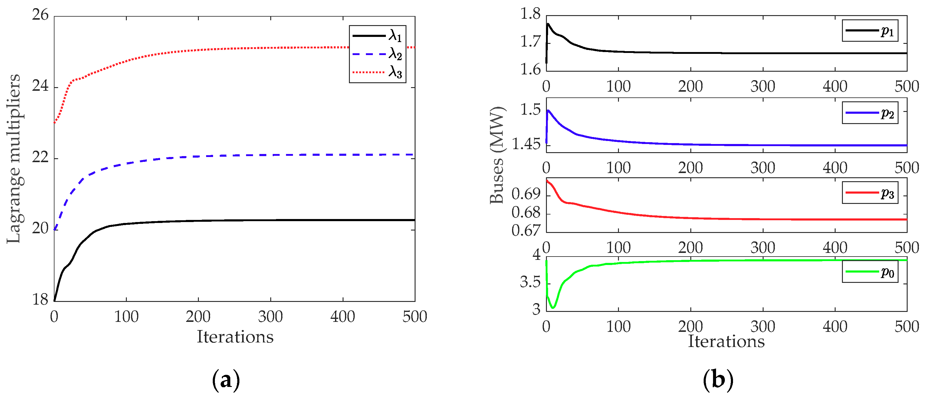
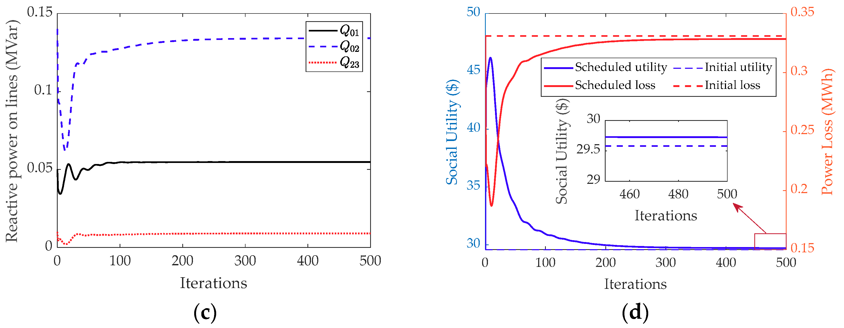
Then, we tested the distributed algorithm mentioned above in MATLAB using the CVX toolbox. The penalty coefficient of the difference between initial demand ${\widehat{p}}_i$ and final supply $p_i$, ${\mathsf{\alpha }}_i$, was 10, 20 and 50, respectively, for each bus. The Lagrange multipliers for the active power equality constraints are depicted in Figure 7a. Because there is power loss term in the objective function, the Lagrange multipliers are not the real electricity price. They are called the shadow prices, and can be used as signals to coordinate the trade. Figure 7b is the real power demand and supply on each bus. The iterations of reactive power on lines are shown in Figure 7c. Figure 7d is the convergence of the social utility and power loss. The optimized system data are shown in

Table 4. Optimized bus data.

Bus	Voltage	Generation		Demand
	Mag (pu)	P (MW)	Q (MVAr)	P (MW)	Q (MVAr)
0	1.0000	3.9455	0.1904	-	-
1	0.9356	-	-	1.6696	0
2	0.9117	0.1890	0	1.4546	0
3	0.8734	-	-	0.6794	0

and

Table 5. Optimized branch data.

Branch	Branch Power		Loss
	P (MW)	Q (MVAr)	P (MW)	Q (MVAr)
0–1	1.7837	0.0522	0.1141	0.0522
0–2	2.1617	0.1351	0.1871	0.1260
2–3	0.7091	0.0091	0.0297	0.0091
		Total:	0.3309	0.1873

.

Table 6. Comparison of original and optimized case in 1 h.

Case	Bus Total Utility ($)	Cost ($)	Social Utility ($)	Power Loss (MWh)
Original	82.2364	52.5305	29.7059	0.3310
Centralized optimized	82.6543	52.9082	29.7461	0.3309
Distributed optimized	82.6543	52.9082	29.7461	0.3309

compares the cost and utility of the original system and the optimized system. It is clear that, after the optimization, the social utility is more and the power loss is less. Additionally, the distributed algorithm can achieve the optimization solution as the central algorithm.

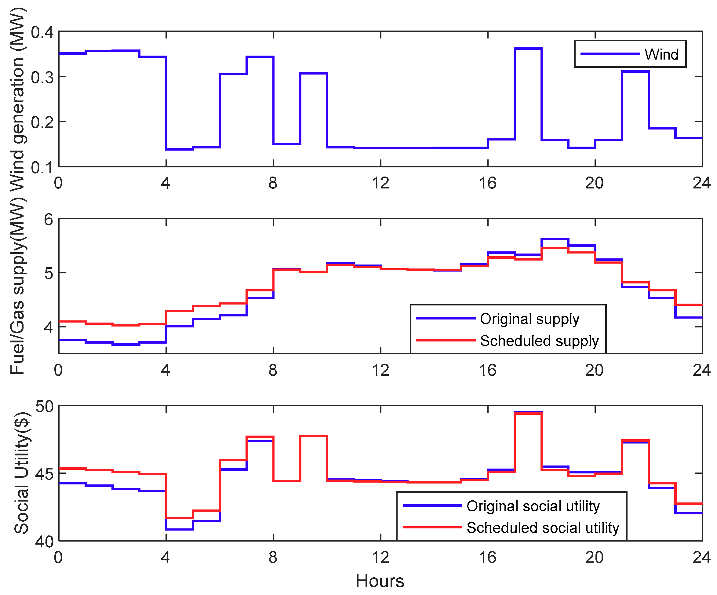
The optimized energy trading is compared with the original trading in 24 h, as depicted in Figure 8. We can see that the wind power generation has a great influence on the system utility. The more that wind generation is injected to the grid, the greater the social utility that is achieved. Moreover, the trading mechanism encourages trading during the low valley of electricity consumption and represses trading during the peak period. The peak cutting and valley filling performance of the proposed trading mechanism is beneficial for the microgrid.

5. Conclusions

In this paper, a distributed energy trading management has been proposed to optimize the utility of a microgrid. When compared with existing publications, the demand of each LV distribution network is forecasted by the ANN method rather than given in advance. Additionally, in the optimization of energy trading, the power flow constraints and power loss minimization are included, rather than only the optimizing active power. The distributed PCPM algorithm guarantees that the operators in microgrid only need to negotiate with neighbors instead of sharing information to all. Finally, the simulation of a four-bus microgrid with practical data demonstrates the effectiveness of the proposed scheme.

It should be noted that the reactive power compensation is not considered in the energy trading management. Additionally, the trading in the LV distribution network of each bus is not included. In the future, the study of hierarchically distributed energy trading management with reactive power compensation can be continued.

References

- Flores-Quiroz, A.; Palma-Behnke, R.; Zakeri, G.; Moreno, R. A column generation approach for solving generation expansion planning problems with high renewable energy penetration. Electr. Power Syst. Res. 2016, 136, 232–241. [Google Scholar] [CrossRef]
- Liu, C.; Chau, K.T.; Zhang, X. An Efficient Wind–Photovoltaic Hybrid Generation System Using Doubly Excited Permanent-Magnet Brushless Machine. IEEE Trans. Ind. Electron. 2010, 57, 831–839. [Google Scholar] [CrossRef]
- Gao, S.; Chau, K.T.; Liu, C.; Wu, D.; Chan, C.C. Integrated Energy Management of Plug-in Electric Vehicles in Power Grid With Renewables. IEEE Trans. Veh. Technol. 2014, 63, 3019–3027. [Google Scholar] [CrossRef]
- Li, Y.; Zhao, T.; Liu, C.; Zhao, Y.; Yu, Z.; Li, K.; Wu, L. Day-Ahead Coordinated Scheduling of Hydro and Wind Power Generation System Considering Uncertainties. IEEE Trans. Ind. Appl. 2019, 55, 2368–2377. [Google Scholar] [CrossRef]
- Jiaqiang, E.; Liu, G.; Liu, T.; Zhang, Z.; Zuo, H.; Hu, W.; Wei, K. Harmonic response analysis of a large dish solar thermal power generation system with wind-induced vibration. Sol. Energy 2019, 181, 116–129. [Google Scholar]
- Li, J.; Chau, K.T.; Jiang, J.Z.; Liu, C.; Li, W. A New Efficient Permanent-Magnet Vernier Machine for Wind Power Generation. IEEE Trans. Magn. 2010, 46, 1475–1478. [Google Scholar] [CrossRef]
- Liu, G.; Ollis, T.B.; Xiao, B.; Zhang, X.; Tomsovic, K. Distributed energy management for community microgrids considering phase balancing and peak shaving. IET Gener. Transm. Distrib. 2019, 13, 1612–1620. [Google Scholar] [CrossRef] [Green Version]
- Zou, Y.; Dong, Y.; Li, S.; Niu, Y. Multi-time hierarchical stochastic predictive control for energy management of an island microgrid with plug-in electric vehicles. IET Gener. Transm. Distrib. 2019, 13, 1794–1801. [Google Scholar] [CrossRef]
- Liu, C.; Chau, K.T.; Diao, C.; Zhong, J.; Zhang, X.; Gao, S.; Wu, D. A new DC micro-grid system using renewable energy and electric vehicles for smart energy delivery. In Proceedings of the 2010 IEEE Vehicle Power and Propulsion Conference, Lille, France, 1–3 September 2010; pp. 1–6. [Google Scholar]
- Liu, C.; Zhong, J.; Chau, K. An intelligent DC micro-grid system for smart energy delivery with plug-in BEVs and HEVs. In Proceedings of the International Electric Vehicle Symposium, EVS-25, Shenzhen, China, 5–9 November 2010. [Google Scholar]
- Xia, Y.; Wei, W.; Yu, M.; Peng, Y.; Tang, J. Decentralized Multi-Time Scale Power Control for a Hybrid AC/DC Microgrid With Multiple Subgrids. IEEE Trans. Power Electron. 2018, 33, 4061–4072. [Google Scholar] [CrossRef]
- Meus, J.; Poncelet, K.; Delarue, E. Applicability of a Clustered Unit Commitment Model in Power System Modeling. IEEE Trans. Power Syst. 2018, 33, 2195–2204. [Google Scholar] [CrossRef]
- Wu, D.; Chau, K.T.; Liu, C.; Gao, S. Genetic Algorithm Based Cost-emission Optimization of Unit Commitment Integrating with Gridable Vehicles. J. Asian Electr. Veh. 2012, 10, 1567–1573. [Google Scholar] [CrossRef]
- Chen, G.; Li, C.; Dong, Z. Parallel and Distributed Computation for Dynamical Economic Dispatch. IEEE Trans. Smart Grid 2017, 8, 1026–1027. [Google Scholar] [CrossRef]
- Hayes, B.; Melatti, I.; Mancini, T.; Prodanovic, M.; Tronci, E. Residential Demand Management Using Individualized Demand Aware Price Policies. IEEE Trans. Smart Grid 2017, 8, 1284–1294. [Google Scholar] [CrossRef]
- Cobos, N.G.; Arroyo, J.M.; Street, A. Least-Cost Reserve Offer Deliverability in Day-Ahead Generation Scheduling Under Wind Uncertainty and Generation and Network Outages. IEEE Trans. Smart Grid 2018, 9, 3430–3442. [Google Scholar] [CrossRef]
- Hong, T.; Fan, S. Probabilistic electric load forecasting: A tutorial review. Int. J. Forecast. 2016, 32, 914–938. [Google Scholar] [CrossRef]
- Xu, F.Y.; Cun, X.; Yan, M.; Yuan, H.; Wang, Y.; Lai, L.L. Power market load forecasting on neural network with beneficial correlated regularization. IEEE Trans. Ind. Inform. 2018, 14, 5050–5059. [Google Scholar] [CrossRef]
- Kunwar, N.; Yash, K.; Kumar, R. Area-load based pricing in DSM through ANN and heuristic scheduling. IEEE Trans. Smart Grid 2013, 4, 1275–1281. [Google Scholar] [CrossRef]
- Liu, D.; Sun, Y.; Qu, Y.; Li, B.; Xu, Y. Analysis and Accurate Prediction of User’s Response Behavior in Incentive-Based Demand Response. IEEE Access 2018, 7, 3170–3180. [Google Scholar] [CrossRef]
- Liu, Y.; Yuen, C.; Hassan, N.U.; Huang, S.; Yu, R.; Xie, S. Electricity Cost Minimization for a Microgrid With Distributed Energy Resource Under Different Information Availability. IEEE Trans. Ind. Electron. 2015, 62, 2571–2583. [Google Scholar] [CrossRef]
- Li, C.; Bosio, F.d.; Chen, F.; Chaudhary, S.K.; Vasquez, J.C.; Guerrero, J.M. Economic Dispatch for Operating Cost Minimization Under Real-Time Pricing in Droop-Controlled DC Microgrid. IEEE J. Emerg. Sel. Top. Power Electron. 2017, 5, 587–595. [Google Scholar] [CrossRef]
- Chen, F.; Chen, M.; Li, Q.; Meng, K.; Zheng, Y.; Guerrero, J.M.; Abbott, D. Cost-Based Droop Schemes for Economic Dispatch in Islanded Microgrids. IEEE Trans. Smart Grid 2017, 8, 63–74. [Google Scholar] [CrossRef]
- Valdez, F.; Melin, P.; Castillo, O. An improved evolutionary method with fuzzy logic for combining particle swarm optimization and genetic algorithms. Appl. Soft Comput. 2011, 11, 2625–2632. [Google Scholar] [CrossRef]
- Precup, R.E.; David, R.C.; Petriu, E.M.; Szedlak-Stinean, A.I.; Bojan-Dragos, C.A. Grey wolf optimizer-based approach to the tuning of PI-fuzzy controllers with a reduced process parametric sensitivity. IFAC-PapersOnLine 2016, 49, 55–60. [Google Scholar] [CrossRef]
- Abed-alguni, B. Island-based Cuckoo Search with Highly Disruptive Polynomial Mutation. Int. J. Artif. Intell. 2019, 17, 57–82. [Google Scholar]
- Shams, M.; Rashedi, E.; Dashti, S.; Hakimi, A. Ideal gas optimization algorithm. Int. J. Artif. Intell. 2017, 15, 116–130. [Google Scholar]
- Farivar, M.; Low, S.H. Branch flow model: Relaxations and convexification—Part I. IEEE Trans. Power Syst. 2013, 28, 2554–2564. [Google Scholar] [CrossRef]
- Li, N.; Chen, L.; Low, S.H. Optimal demand response based on utility maximization in power networks. In Proceedings of the 2011 IEEE Power and Energy Society General Meeting, Detroit, MI, USA, 24–29 July 2011; pp. 1–8. [Google Scholar]
- Chung, K.H.; Kim, B.H.; Hur, D. A new approach to generation scheduling in interconnected power systems using predictor-corrector proximal multiplier method. Electr. Eng. 2012, 94, 177–186. [Google Scholar] [CrossRef]
- Kim, B.H.; Baldick, R. A comparison of distributed optimal power flow algorithms. IEEE Trans. Power Syst. 2000, 15, 599–604. [Google Scholar] [CrossRef]
- ISO New England (ISO-NE) Home Page. Available online: https://www.iso-ne.com/ (accessed on 4 September 2019).
- Glover, J.D.; Sarma, M.S.; Overbye, T. Power System Analysis & Design; SI Version; Cengage Learning: stamford, CT, USA, 2012. [Google Scholar]
- Independent Electricity System Operator (IESO) Home Page. Available online: www.ieso.ca/ (accessed on 4 September 2019).
- Matpower Home Page. Available online: https://matpower.org/ (accessed on 4 September 2019).
Figure 1.
The microgrid framework.
Figure 2.
Distribution line model.
Figure 3.
Artificial neural network (ANN) structure.
Figure 4.
Microgrid single line diagram.
Figure 5.
Process of evaluation.
Figure 6.
Hour-ahead demand forecast results by ANN. (a) Demand forecast results of a whole year; (b) Demand forecast results of two weeks; (c) Forecast error distribution; (d) Breakdown of forecast error statistics by hour.
Figure 7.
Operation results of the distributed energy trading algorithm. (a) Trajectories of the Lagrange multipliers; (b) Trajectories of real power on buses; (c) Trajectories of reactive power on lines; (d) Trajectories of social utility and power loss.