Improved Control of Radiator Heating Systems with Thermostatic Radiator Valves without Pre-Setting Function


1
Vlaamse Instelling voor Technologisch Onderzoek VITO NV, Boeretang 200, 2400 Mol, Belgium
2
EnergyVille, Thor Park 8310, 3600 Genk, Belgium
3
Department of Civil Engineering, Technical University of Denmark, Brovej, Building 118, DK-2800 Kgs. Lyngby, Denmark
*
Author to whom correspondence should be addressed.
Energies 2019, 12(17), 3215; https://doi.org/10.3390/en12173215
Submission received: 18 July 2019
/
Revised: 12 August 2019
/
Accepted: 17 August 2019
/
Published: 21 August 2019
(This article belongs to the Section G: Energy and Buildings)
Abstract
:Low-temperature district heating will play an important role in a future free of fossil fuels. This will only be able to be realized through the low-temperature operation of heating systems in existing buildings. Existing radiator systems can operate with low temperatures for most of the year because they are designed for extremely cold days, but errors have to be corrected and the control of the radiator systems needs to be improved. In this paper, we present a strategy to achieve low-temperature operation from the radiator system of a multi-family building in Denmark without a pre-setting function in the thermostatic radiator valves. The strategy is based on operating the system with a combination of a minimum supply temperature and small temperature differences over the radiators. The operation of the system is analyzed through a thermal-hydraulic model. A minimum supply temperature weather compensation curve was calculated and implemented in the central supply temperature control. Return temperature measurements in the substation, the risers, and several critical radiators were performed before and after the implementation of the strategy. The measurements confirm that a lower supply temperature results in a reduction of the return temperature. However, the system operator needs to be supported by a tool package to correctly maintain the system’s operation.
1. Introduction
Of the overall energy used by the European Union’s (EU) households, 79% is used for space heating (SH) and domestic hot water (DHW) applications [1]. The building sector in the EU is heated by individual heat sources installed in buildings or by using district heating (DH) networks. DH networks are mainly used in Scandinavian and Eastern European countries [2]. DH comprises a network of pipes connecting the buildings of an area to centralized plants. The DH systems allow large scale fossil-free sources of heat to be used: Waste heat from industrial processes and heat produced locally from renewable energy sources (RES) such as biomass, geothermal or solar energy, and heat pumps [3]. However, the heat market of the EU’s buildings is dominated by fossil fuel-based individual boilers, which amounts to approximately 66% of the heat supply [4]. Replacing the individual fossil-fuel boilers through establishing or expanding DH networks based on non-fossil fuels could lead to the reduction of greenhouse gas emissions and help reach the EU goals for a fossil-fuel-free society by 2050, if not sooner [5,6,7].
According to Heat Roadmap Europe [4], DH will play an important role in the implementation of RES into energy systems in the future. To achieve this, DH temperatures must be reduced. The current third generation of DH systems, or medium-temperature DH (MTDH), is defined by typical DH supply and return temperatures of 85 and 45 °C, respectively. In the future fourth generation of DH systems, or low-temperature DH (LTDH) systems, the DH supply and return temperatures must be reduced to 55 and 25 °C, respectively, at the primary side of the building substations.
The transition to LTDH can be done through two different paths, in two steps (Figure 1) [8]. Step 1a is the reduction of the DH return temperature to 25 °C, without reducing the supply temperature. The benefits of choosing this path are the higher heat production efficiency of the biomass combined heat and power plants, or other heat production plants, due to the higher efficiency of the flue gas condensation, the lower distribution heat losses and the increased capacity of the existing network. This step is relevant for newly-built biomass boilers with lifetimes of several decades. Step 1b is the reduction of the DH supply temperature to 55 °C, resulting in a small reduction of the DH return temperature to 35 °C. The benefit of choosing this second path is the higher heat production efficiency for DH systems where central heat pumps are used, due to the higher coefficient of performance of the heat pumps below 60 °C. Additional benefits are the lower distribution losses and the utilization of waste heat. When the operation of the heating systems is further improved, they can operate with supply and return temperatures of 55 and 25 °C respectively. This makes it possible to implement the LTDH system.
Only through the low-temperature operation of both SH and DHW systems inside buildings will it be possible to realize LTDH. However, the heat exchangers between the primary DH network and the secondary space heating system, in the case of indirect systems, have to be designed and operating without faults. The optimal operation of the heat exchangers, by providing a small temperature difference between the primary and the secondary system, will result in low DH temperatures [9,10]. This article is focused only on improving the operation of the SH systems of existing buildings. Existing buildings will remain the major part of the building stock in the future due to the lifetime of buildings.
According to literature, [2,8,11,12,13], it is possible to operate the SH systems of existing buildings with low supply temperatures during most of the year. The SH systems in existing buildings are generally dimensioned for ambient temperatures that only rarely occur, and they are large enough to ensure proper thermal comfort for lower supply temperatures. However, the control of the SH system needs to be improved to ensure a low return temperature, and possible errors have to be identified and corrected.
The aim of this article is to test two control strategies for a radiator SH system in existing multi-family buildings, with no pre-setting function in the thermostatic radiator valves (TRVs) in order to reduce the operating temperatures. These two control strategies are based on the SH system operation under high supply temperature and low mass flow circulation rate, and low supply temperature and high circulation mass flow rate, applied in radiator systems without a pre-setting function and with the sufficient pump differential pressure required in the system.
Radiator systems are the most common SH configuration in existing buildings. The heat emitted from a radiator is defined by the logarithmic mean temperature difference (LMTD) between the radiator and the indoor air temperature. LMTD is dependent on both the supply and the return temperature of the water through the radiator. Different combinations of supply and return temperature can provide the same LMTD. The supply temperature can be controlled centrally in the substation. The return temperature can be controlled by the TRVs that will adjust the mass flow rate through the radiator [2].
The supply temperature of the SH system is commonly controlled according to a weather compensation curve. It must be realized that the existing SH systems are designed based on specific extremely low ambient conditions, without taking into account solar and internal gains [12,13]. These conditions are called designed conditions. In Denmark, the designed conditions are defined by Danish Standards 418 [14]: −12 °C ambient temperature, 0% solar and internal gains, and 20 °C indoor temperature. The ambient temperature is higher than the design temperature during the year, and the solar and internal gains provide free heat. Therefore, the heating demand decreases compared to the design conditions. To restore the heat balance under these part load conditions, the heat emitted from the radiators must be reduced. One way is to reduce the supply temperature. The weather compensation curve relates a specific supply temperature set point with a specific ambient temperature. As the ambient temperature increases, the supply temperature set point decreases. The ambient temperature is recorded by a sensor and the signal from the sensor is used for the adjustment of the supply temperature in the controller [15]. However, the internal heat gains and the solar gains are specific for each individual room and therefore an individual control on each radiator is necessary. This individual control of the radiator that guarantees the comfort temperature in every room is provided by the TRV, which limits the flow rate through the radiator to control the heat output [2].
The mass flow distribution according to the energy requirements of different rooms is dependent on the mass flow balancing of the radiator system. A radiator system is balanced when there is the right differential pressure across every radiator valve that ensures the right mass flow rate for the relevant part load operation [16]. The circulation pump of the system must provide the minimum differential pressure to ensure the required pressure difference and mass flow rate in the system for the relevant part load conditions. The flow balancing of the system may be obtained by correctly used TRVs, but typically needs to be ensured with the use of supplementary functions, such as TRVs with adjustable pressure drop functions. This is a mass flow limitation function, typically referred to as ‘valves with pre-setting’, or pressure independent ‘dynamic valves’. However, in many older buildings without renovation measures applied, TRVs without pre-setting functions are typically used.
A system where the supply temperature is kept high and the mass flow is regulated effectively by the TRVs can be considered as a low-flow system. The low-flow system can lead to a very low pressure drop in the system and all the TRVs can work with almost the same pressure drop [15]. It has been proven [17] that the low-flow system can lead to the lowest return temperature and that the operation of the TRVs is more efficient. However, it requires that the TRVs always operate properly in order to regulate the mass flow to low levels [18].
On the other hand, when the supply temperature is reduced, the mass flow allowed by the TRVs will be increased to provide the required heat output. This will result in a smaller cooling of the water and a higher required pump differential pressure, due to the overall increase of the mass flow in the system. This can be considered a high-flow system [15]. The benefit of operating the system as a high-flow system is that in cases of extensive problematic operation of the TRVs, the uncontrolled flow in the system will not lead to a severe increase of the return temperature, due to the limitation of the supply temperature. If the designed cooling of the water is small, the increase of the return temperature cannot be higher than the cooling of the water. In most building installations, adjusting the mass flow to a low- or high-flow system can easily be achieved by adjusting the control of the circulation pump.
In Denmark, the balancing of the radiator systems in existing buildings depends on the optimal operation of the TRVs with a pre-setting function. However, older buildings are not equipped with TRVs with a pre-setting function. The problem becomes more significant when the operation of the TRVs is problematic. There are several studies [12,19,20,21,22,23,24,25] indicating that the optimal operation of the TRVs is affected by faults and misuse by the users. Several fully opened TRVs can cause an imbalance in the system: If the radiator in the lowest position of a riser in a multi-family building has a fully open TRV, a high flow can run through the radiator with a very small pressure drop. The flow in the whole loop of pipes through the lowest radiator increases to balance the pressure drop in the loop with the pressure difference of the pump. The result will be that the radiators in the higher positions of the risers will not have enough pressure drop to ensure the minimum required mass flow. The lack of balancing in the system will result in some radiators with a higher mass flow than necessary and other radiators in critical positions will not have enough mass flow to ensure the required thermal comfort. The lack of thermal comfort gives rise to complaints directed to the operators by the users of the SH systems of the building. This problem is more significant in multi-family buildings due to the risk that the fully opened TRVs in one flat can result in insufficient flow and heating in radiators in other flats.
In order to restore the thermal comfort in the critical rooms, SH system operators in Denmark typically increase the pump differential pressure or the supply temperature. This attempt to solve the problem without fixing the problematic TRVs in the system may stop complaints, but may also cause more problems in the system. The higher supply temperature will ensure the required heat output from the critical radiators but will cause a high return temperature in the radiators with the higher mass flow. The higher pressure difference of the pump will ensure the required pressure difference and mass flow in the critical radiators. However, the excess pressure difference in the fully open TRVs of some radiators will cause a significant increase in the mass flow in the system resulting in high return temperature and noise problems.
In the literature, several control strategies are proposed to achieve low return temperatures from the operation of radiator SH systems. A new adaptive control algorithm for the operation of the radiator system employs an optimal combination of supply temperature and a low variable mass flow in the overall system to achieve the lowest return temperature [26,27]. This control algorithm is independent of the use of TRVs in the system, but they must be operated without faults to provide the correct heat demand to different rooms. However, it was uncertain if the operation of the TRVs under the tests of this control algorithm was sufficient to provide the necessary mass flow limitation in the radiators. The possibility of using the DH supply temperature instead of the ambient temperature for the control of the SH supply temperature has been proposed [28] and evaluated [29]. However, in this control strategy, it is not examined if the mass flow in each radiator in the system is sufficient to maintain thermal comfort. Instead, the overall mass flow of the system is taken into account. In a different study [19], it was proposed that daily adjustments of the SH supply temperature by using the system mass flow as feedback can accommodate the changes in heat demand and keep the system mass flow in an appropriate range. However, this strategy was also dependent on the proper setting of TRVs with a pre-setting function.
All the previous control strategies succeeded because the radiator systems were balanced and the TRVs were equipped with pre-setting functions. However, in older buildings, the problematic operation of the TRVs that are not equipped with pre-setting function can result in a lack of balance in the radiator systems. As a result, the previous strategies cannot be applied in the imbalanced radiator systems of older buildings.
This article presents new knowledge, as improved control with lower operating temperatures and a minimum temperature difference between supply and return temperature for radiator systems without pre-setting functions has not been described in the literature.
2. Case Study
The building selected as a case study was constructed in 1970 and is located in Viborg, Denmark. The building is heated by DH through a central substation located in the basement. The building includes an unheated basement and three floors with 33 apartments in total. The total heated floor area is 2625 m2. The building constructions consist of a flat roof with 100 mm insulation, exterior cavity brick/concrete walls, and windows with either new two-layer energy glazing or older double glazing. There is no mechanical ventilation in the building.
The SH system consists of a two-string radiator system (Figure 2). There are 173 radiators in the building, connected by 32 risers to the main distribution pipes in the basement. The control of the substation is regulated by an ECL 310 controller, which allows detailed settings of a weather compensation-based supply temperature curve. The supply temperature to the heating system is set at 50 °C for an ambient temperature of 0 °C. The circulation pump of the system is a Grundfos MAGNA pump and it can provide a constant pressure difference to the system that can be set manually in the range up to 100 kPa under three operation modes. Each radiator is equipped with a TRV valve with no pre-setting function. As a result, the hydraulic balance of the building is poor. The design heating capacity of each radiator is according to the operation conditions of 70/40/20 °C. The total design heat output of the radiator system is 89 kW. The DHW system of the building case study is not described as it is not part of the investigation related to this article.
The basic characteristic of this building case study was the high return temperature from the radiator system. In Figure 3, the daily average DH supply and return temperature, along with the daily average energy use for SH, measured by the main energy meter in the substation, are illustrated for 2017.
In Figure 4, the daily part load operation of the SH system of the building case study for all days in 2017 is shown as a duration curve, whereby 100% represents the design heat load of the system. The part load operation was calculated from the daily average energy use for SH, divided by the total design heating capacity of the radiator system. The daily part load operation was higher than 60% for only 10 days during 2017. In Figure 5, the daily part load operation of the SH system is illustrated in relation to the ambient temperature for each day of 2017.
The energy and temperature data recorded by the energy meter of the building case verify the potential of using low-temperature operation for SH, as it is described in the Introduction. More specifically, the actual part load operation of the radiator system is significantly lower than the designed conditions during most of the heating season. In addition, the DH return temperature is significantly high during most of the year period.
3. Methodology
3.1. Overview of the Research Procedure
As it is stated in the aim of this article, two different strategies were investigated to reduce the temperature levels of the radiator system. The first strategy was focused on operating the radiator system with a high supply temperature and a low differential pump pressure, by also improving the individual control of the radiators of the building case, through identifying and fixing errors and teaching the users how to operate the TRVs efficiently. The second strategy was focused on operating the radiator system with a low supply temperature and a higher differential pump pressure, by limiting the effect of the existing errors in the control of the radiators. The two strategies are illustrated in Table 1.
The investigation process was based first on analyzing the two strategies through a thermal-hydraulic model of the radiator system of the building case, to identify how the suggested strategies could reduce the return temperature in case of no problematic TRVs in the system and in case of several TRVs that cannot regulate the mass flow through the radiators. Then, the investigation was focused on testing the two strategies in the real building case.
3.2. Equations Describing the Operation of the Heating System Used for the Creation of the Thermal-Hydraulic Model
The hydraulic configuration of the radiator double string system consists of two different pipelines: one is the supply and the other is the return line. Hot water from the supply pipeline enters the radiator from a top corner and flows horizontally in the top header and vertically down the plate while it cools gradually, before exiting the radiator at the lower horizontal header [6]. The equations presented in this section describe the operation of the heating system and are used for the construction of the thermal-hydraulic model for the analysis.
Each riser of the system is modeled as a loop from the position of the pump to the end of the riser. Several pipe sections of the main distribution pipes in the basement are part of many different loops. As a result, the mass flow and the pressure drop in different pipe sections are affected by the differential pressure of the pump, the mass flow requirements, and the pressure drop of several loops and radiators.
The thermal-hydraulic model is designed to calculate first as a reference condition the required mass flow rate () and pressure drop () across each radiator, each pipe section, and the overall radiator system, for both design and part load conditions, under the ideal operation of the system without errors. The design heat output () of each radiator in the system and the design supply and return temperatures are provided by the SH system operator and they are used as inputs for this calculation.
The heat transfer from the water in the pipes to the radiator element is described as:
where the mass flow () is the only unknown in the system. is the heating capacity of the water. Equation (1) applies to both design and part load conditions. The logarithmic mean temperature difference () between the radiator and the indoor air is given by the equation:
where is the indoor temperature. The part load operation () is defined as the fraction of the actual heat output of the radiator () to the design heat output ():
where corresponds to the design conditions and corresponds to the actual part load conditions. The radiator exponent () describes the exponential relationship between the mean temperature difference and the heat emitted from the radiator. A typical value of the radiator exponent for hydraulic radiators is 1.3 [2]. The mass flow required for each radiator is calculated from Equation (1) when the heat output of the radiator () is known at each part load. The velocity of the heat carrier () in each pipe section is calculated from the equation:
where is the mass flow at each pipe section and di is the diameter of the pipe section.
The calculation of the friction factor () for each pipe section is dependent on the type of flow inside the pipe. The type of flow is defined by the Reynolds number () for each pipe section, which is calculated as:
where ρ is the density and is the dynamic viscosity of the water. In the case of laminar flow, the Reynolds number should be lower than 2000 and the friction factor is calculated by using the Hagen–Poiseuille equation:
For a Reynolds number between approximately 2000 and 4000, there is a transition area from laminar flow to turbulent flow. For Reynolds number values higher than 4000, the flow is fully turbulent. For the calculation of the friction factor in the transitional area and for turbulent flow, the Colebrook–White equation is used. However, to calculate the friction factor without the necessary iterations of the Colebrook–White equation, the Swamee–Jain Equation (8) can be used instead. This equation gives a good approximation of the Colebrook–White equation [30]:
where e is the roughness of each pipe section.
As a result, the pressure drop of each pipe section () is calculated as the total pressure drop loss of both the supply and return pipe:
where is the minor pressure drop, i.e., the sum of the local pressure drops resulting from the specific fitting of the pipes, and is the length of both the supply and return pipe of each pipe section.
Each of the radiators is equipped with a radiator valve. To ensure the correct functioning of the valves, a certain pressure drop ( is set in each of them. The flow coefficient ) relates the mass flow and the pressure drop across the valve according to the equation:
The flow coefficient can get a different value if the valve is equipped with a pre-setting function in order to reduce the maximum available flow through the valve. When the valve is not equipped with a pre-setting function, like the building case examined, the flow coefficient receives the maximum value of ) defined by the manufacturer.
The minimum required pressure difference of the pump at each part load is equal to the pressure drop from the position of the pump up to the critical radiator of the system, according to the equation:
Which is the sum of the total pressure drop of the pipe sections in the critical route of the system (), the additional pressure drop caused across the valve in the critical radiator (), and the minimum pressure drop required for the optimal operation of the TRV mounted on the critical radiator which is usually 10 kPa. The pressure drop across the valve () is dependent on the flow coefficient () of the valve and is calculated from Equation (9).
Under part load operation conditions, the required mass flow and the pressure drop of the system are lower. Under these conditions, the type of pump used is quite important. When a fixed high differential pressure is used it results in a high flow through the open TRVs based on the equation:
On the other hand, when the pressure difference of the pump can be adjusted to the minimum required, the pressure difference over the TRVs is not more than needed for a good control function.
After the calculation of the mass flow and the pressure difference of the system under the ideal operation without errors, the model is designed to calculate the new mass flow rate and the pressure difference of the system for a scenario where there are TRVs that cannot regulate the mass flow through several radiators in the system.
When one or more TRVs in the system cannot regulate the mass flow through the radiators, an imbalance situation occurs, resulting in uncontrolled flows in the system. According to Equations (1)–(3), each radiator has an ideal controlled mass flow under each part load condition. When there is no flow regulation through the TRV, the uncontrolled flow is different than the ideal. This uncontrolled flow has to be calculated based on the hydraulic balance of the loop. If multiple uncontrolled flows exist in different loops, they have to be calculated iteratively based on the hydraulic balance of the system. Each uncontrolled mass flow rate () from a radiator in the system is calculated according to the equation:
The sum of the pressure drop in the loop until the radiator () is affected by the mass flow increase in several pipe sections due to uncontrolled flows in different loops. For radiators in the system with TRVs that are still able to regulate the mass flow, the ideal mass flow required remains the same.
The tool for the iterative calculation was Visual Basic for Applications (VBA) in Excel. The iterative calculation was performed calculating the uncontrolled mass flow in all loops, one-by-one, and making use of the results in the following mass flow calculation. The iterative calculation process was typically repeated 30 times and ended when the changes in the mass flow calculation from one iteration to the next iteration were insignificant. There are commercial software packages that can be used to design and dynamically operate a radiator heating system. However, they allow only the design and operation of the system under ideal conditions, without being able to simulate the uncontrolled flow rates due to the problematic operation of the TRVs, which usually occurs under the real operation of the system.
When the mass flow rates for each radiator is recalculated due to the existence of uncontrolled mass flows in the system, the return temperature for each radiator is calculated by solving together Equations (1) and (3) iteratively in the model, by using a solver function, until the following equation is fulfilled:
An overview of the calculation process performed inside the model to determine first the mass flow rate and the minimum required pressure difference of the circulation pump for the radiator system under the case of ideal operation without problematic TRVs and then, under the case of one fully open TRVs that leads into uncontrolled flows in the radiator system are presented in Table 2 and Table 3 respectively.
Due to the different return temperature results at different part load operating conditions, the overall return temperature of the system during the year was also provided as the energy weighted average return temperature (). To calculate the energy weighted average return temperature of the actual building during the heating season, the daily average energy use data of 2017 were used (Figure 3). Nine different half-open intervals were considered from 5% to 95% part load operation with the length of each interval at 10%. The share () of the delivered energy with the actual part load operation inside the selected intervals was calculated during the whole year period. A representative return temperature ( was selected for the middle part load condition of each interval. The energy weighted average return temperature was calculated according to the equation:
3.3. Expected Daily Average DH Return Temperature from the Actual Building Case
Taking into account the daily average DH supply temperature and the daily average energy use for SH during 2017 according to Figure 3, the expected daily average return temperature due to the radiator system operation is calculated by solving Equations (2) and (3) together. This temperature shows what would be the daily average DH return temperature if the operation of the radiator system of the building case examined was ideal, without errors. As a result, this temperature shows the potential to reduce the DH return temperature.
3.4. First Strategy: Low-Flow System Operation
In the first strategy, the low-flow operation of the radiator system was analyzed through model calculations for two different cases: A case of no problematic TRVs in the system and the case of one problematic TRV in each riser, approximately 30 problematic TRVs in the system in total. The first case was a representation of the ideal operation of the radiator system, in order to identify what could be the lowest return temperature and the minimum pump differential pressure required at each part load. The second case was a representation of the typical problematic operation of the radiator system, resulting in uncontrolled flows, defined by the dynamic operation of the overall hydraulic system.
For each part load, the optimal supply temperature was calculated to obtain a return temperature close to the minimum possible. To get a minimum return temperature, a maximum supply temperature is to be used. By accepting a slightly higher return temperature, a much lower supply temperature may be used, especially for the low part load range.
The calculation procedure was based on the principle that a return temperature 2 °C higher than the absolute minimum return temperature would be acceptable. The absolute minimum return temperature was calculated from the model based on the radiator Equations (1)–(3), at each part load for a constant 70 °C supply temperature. Then, the supply temperature was reduced for each part load, until the return temperature was increased by 2 °C.
Based on the optimal supply temperature, the minimum required pump pressure difference for the ideal operation of the radiator system was calculated by the model at each part load through Equations (1)–(11), to ensure a minimum pressure drop of 10 kPa across all the TRVs of the system. This minimum pressure difference of the pump was kept the same for the mass flow calculations of the system in the case of one problematic TRV with the uncontrolled flow in each riser, through Equation (12), in order to ensure at least 5 kPa pressure drop over the most critical TRVs. By ensuring 5 kPa across the critical TRVs, the control of the TRV may be less accurate but can be acceptable.
The overall return temperature for the two different cases and for each part load was calculated by the model, based on Equation (13). Also, the energy weighted average return temperature was calculated for the two cases based on Equation (14).
3.5. Second Strategy: High-Flow System Operation
In the second strategy, the high-flow system operation based on a low supply temperature of the radiator system was analyzed again through model calculations, for the same cases of no problematic TRVs and for one problematic TRV with the uncontrolled flow in each riser. For both cases and for each part load, the low supply temperature was calculated based on two principles.
The first principle was that the cooling of the water in each radiator would be 5 °C. Such a small ΔT between the supply and the return temperature was selected to be able to minimize the supply temperature and to ensure that the increase of the return temperature due to uncontrolled flows would not be higher than 5 °C. The second principle was that the combination of the supply and return temperature selected at each part load should provide an LMTD that would give the required heat output according to the radiator Equations (1)–(3), in order to ensure the thermal comfort. For the calculation of the low supply temperature, a solver function in Excel was used, taking into account the two principles as constraints.
The required pump pressure difference due to the low supply temperature and the high mass flow in the system was calculated by the model at each part load based on Equation (10), for the ideal operation of the heating system. In the case of one problematic TRV in each riser, the pump pressure difference was manually increased to the minimum necessary level in order to ensure the minimum required pressure drop across all the valves in the system.
Once again, for each part load, the overall return temperature for the case of one problematic TRV per riser was calculated by the model, based on Equations (12) and (13). Also, the energy weighted average return temperature was calculated for the two cases based on Equation (14).
3.6. Weather Compensation Curve Proposal
A supply temperature to the radiator system based on a weather compensation curve was proposed for the test of each strategy in the real heating system. Based on the part load operation of the system for each day of 2017, the supply temperature calculated in each strategy for this part load was related to the average daily ambient temperature measured during 2017. Then, through a linear regression analysis, a weather compensation curve was calculated, taking into account only the days of the heating season.
4. Results from Analysis
In Figure 6 the expected DH daily average return temperature due to the ideal operation of the radiator system is illustrated. The monitored DH return temperature is significantly higher than the calculated expected DH return temperature. It is quite clear that the operation of the radiator system is significantly affected by errors related to the insufficient flow regulation by the TRVs and user misuse. These errors lead to a high return temperature from the radiator system. These errors have to be identified and eliminated.
In Figure 7 and Figure 8—the analysis results for the supply and return temperatures—the required pressure difference of the pump and the total mass flow under the low-flow operation of the system are illustrated for the cases without problematic TRVs and with one problematic TRV in each riser. The energy weighted average return temperature for the system without malfunctions was calculated to be 25.1 °C. The return temperature for the case of one open TRV in each riser was calculated to be 46.2 °C. The required pressure difference of the pump for both cases to ensure approximately 10 kPa differential pressure across all the TRVs was almost constant at 11 kPa, for part load operation below 60%.
According to Figure 7, it is clear that the first strategy is quite sensitive to the errors in the system. Under the ideal operation of the system without uncontrolled flows, a supply temperature below 64 °C (at 60% part load conditions) with a return temperature of 30 °C can be applied for most of the heating season. However, in the case of one problematic TRV in every riser, the return temperature curve is significantly higher. In that case, at 60% part load conditions, for the same supply temperature of 64 °C, the return temperature is increased at 50 °C. Figure 7 illustrates the significance of eliminating the errors in the system as a requirement for the success of the first strategy.
In Figure 8, the benefit of the first strategy regarding the control of the circulation pump is illustrated. According to the pump pressure curve, for each part load operation of the system under 60%, a minimum required pressure difference from the pump of approximately 11 kPa is sufficient to ensure the required mass flow in every radiator of the system. As a result, to apply the first strategy in the actual system there is no need to adjust the pressure difference of the pump for most of the heating season. Also, in older buildings, the existing circulation pumps are outdated and they cannot adjust the pressure difference according to the system demands. In these cases, by applying the first strategy there is no need to replace the circulation pump.
In Figure 9, the proposed control of the supply temperature is presented through the linear regression analysis between the required daily average supply temperature for each part load and the ambient temperature recorded during 2017. According to the curve, a supply temperature of 64 °C for an outdoor temperature of 0 °C is sufficient to set the weather compensation based supply temperature controller in the substation.
In Figure 10 and Figure 11—the analysis results for the supply and return temperatures—the required pressure difference of the pump and the total mass flow under the high-flow operation of the system are presented for the cases without problematic TRVs and with one problematic TRV in each riser. In Figure 12, the proposed control of the supply temperature is also presented through a linear regression analysis. The energy weighted average return temperature for the system without malfunctions was calculated to be 33.2 °C. In contrast with the low-flow system, the required pressure difference of the pump for the first case without problematic TRVs was quite proportional to the part load. At 60% of the actual part load operation, the required pressure difference of the pump was approximately 60 kPa.
Under high-flow operation conditions, for the case of one problematic TRV in each riser, the minimum required pressure difference of the pump should be increased, compared to the first case, to ensure a minimum pressure drop of 5 kPa across all the critical TRVs, at least for part load operation below 60%. In the case of one problematic TRV in each riser, the energy weighted average return temperature was calculated to be 35.7 °C and the required pressure difference of the pump at 60% part load operation was 120 kPa.
According to analysis results, the operation of the system under high-flow conditions can provide a low-cost solution to operate the heating system with a supply temperature below 45 °C with an acceptable return temperature of 35 °C for most of the heating season, based on the Viborg case. This solution has less sensitivity to the existence of errors in the system because the increase of the return temperature can be limited by the low supply temperature and the small cooling of the water across the radiators.
Under the high-flow operation conditions, the minimum required pump differential pressure is significantly high and proportional to the part load operation due to the higher mass flow in the system. The minimum required pump pressure difference at each part load is dependent on the number of errors in the system. To ensure the minimum required pressure difference in the system and to avoid excess pressure difference under the lower part load operating conditions, a differential pressure controller must be attached to the critical radiators of the system as a feedback function to the control of the circulation pump. To avoid noise problems due to the higher mass flow in the system, the supply temperature can be increased in order to increase the temperature difference between the supply and the return temperature, and to reduce the mass flow in the system, under higher part load operating conditions.
5. Test of the Two Strategies in the Actual Heating System
5.1. Temperature Measurements in the Substation, the Risers, and the Radiators of a Few Apartments
To test the suggested strategies in the real building case, the operation of the actual radiator system was monitored before and after the implementation of the two strategies. The return temperature of all the risers of the building case was measured at the position where each riser was connected to the main pipeline in the basement. Moreover, the supply and the return temperature were measured on both the primary (DH network) and the secondary (radiator system) side of the heat exchanger in the substation of the building case study. Finally, the return temperature of several radiators was measured in apartments located in the west end of the building. These apartments represent the worst case situation with the highest heat loss due to the gable and the lowest available pressure difference across the valve.
The temperature measurements were performed by using temperature sensors by Sensohive Technologies ApS, equipped with a type K thermocouple wire probes, with tolerances of ±1.5 °C, Class 1. The temperature range between the sensor device and the external measurement is −200 to 1260 °C. The resolution is 0.015. The transmission interval is one transmission every 10 min. Each thermocouple was attached to the relevant pipe section for at least 5 cm. The top was covered with insulation to eliminate the effect of the room temperature in the recording of the accurate temperature of the pipe (Figure 13).
Potential errors between the real temperature of the water in the pipe section and the measured temperature of the pipe surface would have no influence on the overall procedure, because the aim was to detect significant return temperature differences between the different risers and radiators, in order to have an indication of possible errors in the system. The temperature sensors were measuring the temperatures every 10 min. All the data were sent wirelessly to an online database and were accessible for download and further analysis at any time.
5.2. Return Temperature Measurements before Improvements
In Figure 14, the supply and return temperature of the radiator system along with the return temperature of several risers are illustrated from 16 November 2018 to 19 November 2018. The supply temperature of the radiator system (red curve) was fluctuating between 40 and 50 °C, while the return temperature (black curve) was fluctuating between 35 and 40 °C. This initial recording was performed before the implementation of any of the two strategies proposed in the methodology. On 18 November 2018 at 00.00 h and for the previous 1 h, the energy used for the SH system was recorded to be 44 kW. Based on the designed heat load of the radiator system, the actual operation of the system was almost 50%. It is clear (Figure 14) that the return temperature of several risers was only slightly lower than the supply temperature, and that they were following the same variations. This was an indication that there were radiators on these risers that were unable to provide the necessary flow regulation. On the other hand, there were risers with a return temperature significantly lower than the supply temperature, also without following the same variations. The radiators on these risers were either not in operation or they had a mass flow according to the heat demand due to the correct operation of the TRVs. However, the overall return temperature of the radiator system was following exactly the trend of the supply temperature. This was an indication that the risers with a higher return temperature and poor mass flow regulation in the radiators were the dominant part of the system.
During the same period, the return temperature from the radiators of an apartment located at the west end of the first floor of the building case study was measured. According to Figure 15, there is poor flow regulation from the TRVs of the radiators placed in one of the bedrooms and the living room, resulting in a return temperature (black curve) higher than 35 °C. This could be the result of a malfunction in the TRV or due to a higher set point of the thermostat set by the user. On the other hand, the return temperature in the rest of the radiators fluctuates close to 25 °C. The reason for the lower return temperature is that there was either no malfunction in the TRVs and the thermostats were set to a low set point or they were completely turned off. Only the return temperature from the radiator in the kitchen (yellow curve) was increased during the middle of the day of 18 November 2018, because the user increased the set point in the sensor of the TRV.
5.3. Test of the First Strategy: Low-Flow Operation
The first attempt to achieve a reduction of the return temperature was to apply the first strategy of the low-flow system operation in the actual heating system of the building case study, based on the proposed supply temperature curve, in turn, based on the weather compensation control (Figure 9), and the proposed curve for the control of the circulation pump (Figure 8).
Before any changes in the central controller of the supply temperature and the control of the pump, there was an effort to fix the problematic operation of the TRVs in the system by inspecting the apartments with malfunctions in the TRVs. Access to every apartment was not possible due to difficulties in communication with the users and the number of apartments in the building. Nevertheless, a letter was sent to all the users to inform them how to operate their radiators efficiently. The users were recommended to select a set point of 3 in all the thermostats, which represents a desired indoor temperature of 21 °C, and to avoid using night setback. To help them check the return temperature of each of their radiators, they were given a sheet with temperature-sensitive stickers. The stickers had to be attached to the return pipe on every radiator. When the return temperature from a radiator was higher than 30.5 °C, a sad face was shown on the sticker surface, indicating that the return temperature was higher than the desirable level.
To test the first strategy, the radiator supply temperature curve was altered on 26 November 2018 at 12:00 (Figure 16), and the setting of the pump was changed to provide a constant pressure of 20 kPa. The selection of a higher pressure difference than the 11 kPa proposed by the pump was based on the fact that it was not possible to identify the exact number of the faults in the TRVs. To ensure that there would be a pressure drop of at least 5 kPa across each of the functional TRVs, this slightly higher pressure difference was selected.
According to the results (Figure 16), after the implementation of the changes in the control of the radiator supply temperature and the pump operation, there was an increase in both the radiator supply and the return temperature. According to the radiator Equations (1)–(3), under an ideal operation of the TRV, when the supply temperature is increasing the return temperature must be decreasing. As a result, the higher return temperature from the radiator system was an indication that the errors in the system were not eliminated and the operation of the TRVs was still not efficient.
The first strategy of fixing the errors, namely, improving user behavior and operating the system with a high supply temperature to achieve a lower possible return temperature, did not succeed because in practice it is quite difficult to fix every error in the system where there is no pre-setting function in the TRVs and to teach the users to operate their TRVs continuously in an optimal way.
5.4. Test of the Second Strategy: High-Flow Operation
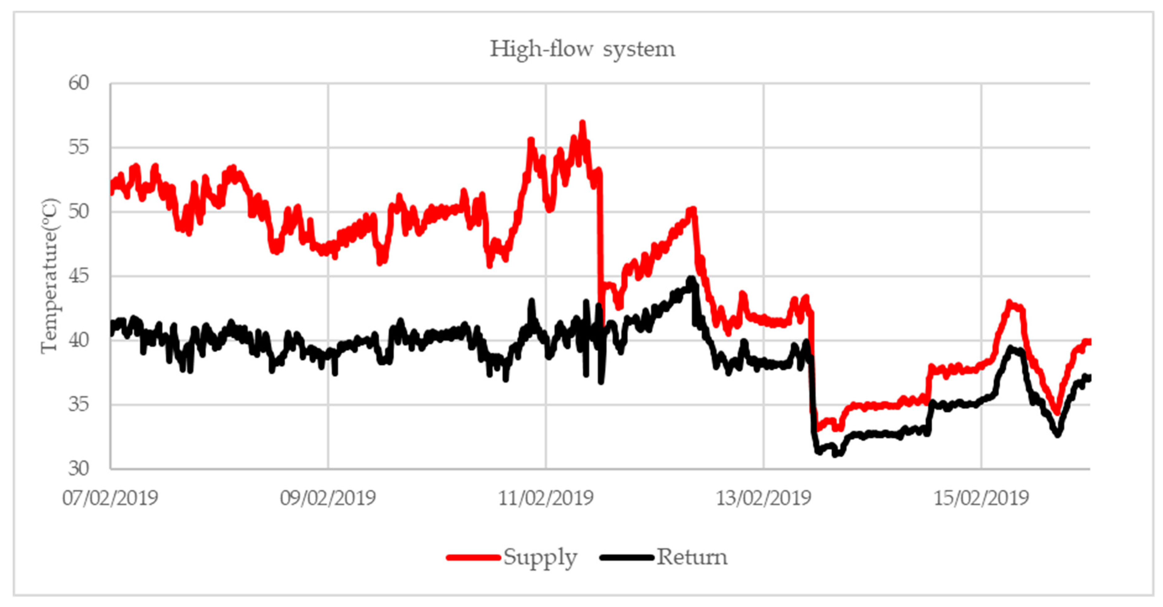
To test the second strategy, there was no further attempt to fix the problematic operation of the TRVs or to improve user behavior. On 11 February 2019, the radiator supply temperature curve was altered and the supply temperature was reduced from 53 °C to 43 °C (Figure 17). At the same time, the pump pressure difference was increased from 20 kPa to 70 kPa to ensure that sufficient flow was delivered. According to the results (Figure 17), there was a reduction in the radiator supply temperature, and the temperature difference between the supply and return temperature was reduced significantly. On 13 February 2019, the radiator supply temperature curve was altered again and the radiator supply temperature was reduced from 43 °C to 34 °C. This reduction in the supply temperature also forced down the return temperature from the radiators.
However, on 14 February 2019, the SH system operator of the building noticed a reduction in the energy delivered from the primary to the secondary side of the heat exchanger. He was concerned that due to this reduction in the energy use for heating there would be complaints from the users regarding poor thermal comfort. To eliminate any possibility of complaints before even they occur, he decided to alter again the supply temperature curve, by increasing the supply temperature from 35 °C to 38 °C. As a result, there was a small increase in the radiator supply temperature that forced up also the return temperature.
According to the overall results, the test of the second strategy showed that both the radiator supply and the return temperature were decreased after the control of the radiator supply temperature and the pump operation were adjusted. Before the changes, the return temperature from the radiators was fluctuating close to 40 °C. After the changes, it was lower than 35 °C, also taking into account the increase of the radiator supply temperature due to the lower ambient temperature. There were no complaints from the occupants regarding their thermal comfort after the changes.
6. Proposal for the Implementation of the High-Flow Strategy
Based on the overall results from the analysis (Section 4) and the test of the proposed strategies in the building case study in Viborg (Section 5), a proposal for implementing the high-flow strategy consisting of four steps is described in this section.
The first step is to identify the potential for the reduction of the supply and the return temperature of the heating system by creating the characteristic operating curves of the heating system, as shown in Figure 3, Figure 4, Figure 5 and Figure 6.
The second step is to calculate the proposed supply temperature curve used in the weather compensation control, according to Section 3.5 and Section 3.6, which is visually depicted in Figure 5 and Figure 11. The supply temperature may be adjusted based on room temperature measurements in critical rooms during the first heating season.
The third step is to set the circulation pump to be controlled by an external differential pressure sensor to continuously provide the minimum required pressure difference at the critical point in the system. This differential pressure sensor must be installed in parallel to the TRV at the top radiator of the riser with the highest mass flow due to a combination of a high number of radiators in the riser and a fully open valve, similar to the TRV, installed between the supply and the return pipe at the basis of the riser, in parallel to the differential pressure sensor. The installed valve ensures that the riser is the critical riser of the system.
The fourth step is to provide the necessary tools to support the SH system operator of the building to deal with complaints from the users regarding thermal discomfort problems. This person must have evidence that the operation of the radiator system is sufficient to provide the required thermal comfort in all rooms. This evidence can be indoor temperatures measured in several rooms of the building, which have been identified as critical. Critical rooms can be rooms with limited solar gain. By using this evidence, the SH system operator can verify that any potential thermal discomfort in the apartments is not due to the low supply temperature to the radiators or low pressure difference from the pump, but due to local errors related to TRVs that are stuck in partially or fully closed positions, air-filled radiators, or radiators that are covered by furniture, or due to the use of only some of the radiators in the apartment to provide the total required heating power of the apartment. The local errors have to be fixed in cooperation between the SH system operator and the complaining users.
7. Discussion
The analysis of the performance of the high flow strategy was based on an actual building case study in Viborg, with relatively large pipe diameters of up to 60 mm in the main distribution pipeline. In newer buildings, smaller pipe dimensions are typically used and therefore the analysis of the high-flow system operation strategy may need to be adjusted before it is used in newer buildings. However, if the buildings are not so old that they have TRVs with pre-setting functions, the use of the high-flow system operation strategy may not be relevant.
The proposed four-step implementation of the strategy was not completely tested. More specifically, the fourth step of the implementation of the necessary tools to help the SH system operator was not tested. However, the potential of using a low supply temperature to secure a low return temperature was demonstrated by analysis and tests. The fourth step will be tested in further work during the following heating season.
8. Conclusions
In this article, methodologies to reduce the temperature levels of the heating system in buildings with a radiator system with TRVs without pre-setting functions were investigated. Two different control strategies were proposed, analyzed, and tested in a multi-family building located in Viborg, Denmark. The two strategies are mainly characterized by the use of a low and high mass flow rate in the radiator system.
The low-flow system operation strategy was not successful because some TRVs were not set correctly, resulting in a high return temperature.
The main results indicate that the operation of the system with high flow and low supply temperature can provide a low-cost solution to operate the radiator system with a supply temperature below 45 °C with an acceptable return temperature of 35 °C for most of the heating season.
However, the SH system operator of the buildings must be supported by the necessary indoor temperature sensors to obtain evidence that the operation of the radiator system is sufficient and that any complaints by the users regarding poor thermal comfort are due to local errors in the specific flats that need to be solved.
Author Contributions
Conceptualization, T.B. and S.S.; methodology, T.B. and S.S.; software, T.B.; formal analysis, T.B.; investigation, T.B.; resources, T.B.; data curation, T.B.; writing—original draft preparation, T.B.; writing—review and editing, R.S., D.V. and S.S.; visualization, T.B.; supervision, R.S., D.V. and S.S.; project administration, T.B.
Funding
This research was funded by VITO NV and Technical University of Denmark, Department of Civil Engineering (DTU_PhD_1701_contract).
Conflicts of Interest
The authors declare no conflict of interest.
References
- European Commission. Energy Efficiency—Heating and Cooling. Available online: https://ec.europa.eu/energy/en/topics/energy-efficiency/heating-and-cooling (accessed on 29 May 2019).
- Tunzi, M.; Østergaard, D.S.; Svendsen, S.; Boukhanouf, R.; Cooper, E. Method to investigate and plan the application of low temperature district heating to existing hydraulic radiator systems in existing buildings. Energy 2016, 113, 413–421. [Google Scholar] [CrossRef]
- Lund, H.; Werner, S.; Wiltshire, R.; Svendsen, S.; Thorsen, J.E.; Hvelplund, F.; Mathiesen, B.V. 4th Generation District Heating (4GDH) Integrating smart thermal grids into future sustainable energy systems. Energy 2014, 68, 1–11. [Google Scholar] [CrossRef]
- Connolly, D.; Lund, H.; Mathiesen, B.V.; Werner, S.; Möller, B.; Persson, U.; Boermans, T.; Trier, D.; Østergaard, P.A.; Nielsen, S. Heat Roadmap Europe: Combining district heating with heat savings to decarbonize the EU energy system. Energy Policy 2014, 65, 475–489. [Google Scholar] [CrossRef]
- European Commission. Europe 2020 Flagship Initiative Innovation Union SEC (2010) 1161; Publications Office of the European Union: Luxembourg City, Luxembourg, 2011. [Google Scholar]
- Analysis of Options to Move Beyond 20% Greenhouse Gas Emission Reductions and Assessing the Risk of Carbon Leakage. Available online: https://eur-lex.europa.eu/legal-content/EN/TXT/?uri=celex%3A52010DC0265 (accessed on 20 August 2019).
- European Commission. A Clean Planet for All. A European Strategic Long-Term Vision for a Prosperous, Modern, Competitive and Climate Neutral Economy COM (2018) 773. Available online: https://eur-lex.europa.eu/legal-content/EN/TXT/?qid=1560755311425&uri=CELEX:52018DC0773 (accessed on 20 August 2019).
- Østergaard, D.S. Heating of Existing Buildings by Low-Temperature District Heating. Ph.D. Thesis, Technical University of Denmark, Department of Civil Engineering, Lyngby, Denmark, 2018. [Google Scholar]
- Gadd, H.; Werner, S. Achieving low return temperatures from district heating substations. Appl. Energy 2014, 136, 59–67. [Google Scholar] [CrossRef] [Green Version]
- Gadd, H.; Werner, S. Fault detection in district heating substations. Appl. Energy 2015, 157, 51–59. [Google Scholar] [CrossRef] [Green Version]
- Østergaard, D.S.; Svendsen, S. Theoretical overview of heating power and necessary heating supply temperatures in typical Danish single-family houses from the 1900s. Energy Build. 2016, 126, 375–383. [Google Scholar] [CrossRef] [Green Version]
- Østergaard, D.S.; Svendsen, S. Experience from a practical test of low-temperature district heating for space heating in five Danish single-family houses from the 1930s. Energy 2018, 159, 569–578. [Google Scholar] [CrossRef]
- Østergaard, D.S.; Svendsen, S. Are typical radiators over-dimensioned? An analysis of radiator dimensions in 1645 Danish houses. Energy Build. 2018, 178, 206–215. [Google Scholar] [CrossRef]
- Danish Standards. DSF/DS 418—Calculation of Heat Loss from Buildings; Danish Standards: København, Denmark, 2011. [Google Scholar]
- Lauenburg, P. Improved Supply of District Heat to Hydronic Space Heating Systems. Ph.D. Thesis, Lund University, Faculty of Engineering, Department of Energy Sciences, Division of Efficient Energy Systems, Lund, Sweden, 2009. [Google Scholar]
- Danish Standards. DS/EN 14336—Heating Systems in Buildings—Installation and Commissioning of Water Based Heating Systems; Danish Standards: København, Denmark, 2005. [Google Scholar]
- Trüschel, A. Hydronic heating systems the effect of design on system sensitivity. Doktorsavhandlingar vid Chalmers Tekniska Högskola 2002, 1857, 1–226. [Google Scholar]
- Monetti, V.; Fabrizio, E.; Filippi, M. Impact of low investment strategies for space heating control: Application of thermostatic radiators valves to an old residential Application of thermostatic radiators valves to an old residential. Energy Build. 2015, 95, 202–210. [Google Scholar] [CrossRef]
- Xu, B.; Huang, A.; Fu, L.; Di, H. Simulation and analysis on control effectiveness of TRVs in district heating systems. Energy Build. 2011, 43, 1169–1174. [Google Scholar] [CrossRef]
- Liao, Z.; Swainson, M.; Dexter, A.L. On the control of heating systems in the UK. Build. Environ. 2005, 40, 343–351. [Google Scholar] [CrossRef]
- Bruce-Konuah, A.; Jones, R.V.; Fuertes, A.; Messi, L.; Giretti, A. The role of thermostatic radiator valves for the control of space heating in UK social-rented households. Energy Build. 2018, 173, 206–220. [Google Scholar] [CrossRef]
- Zinko, H.; Lee, H.; Kim, B.K.; Kim, Y.H.; Lindkvist, H.; Loewen, A.; Ha, S.; Walletun, H.; Wigbels, M. Improvement of Operational Temperature Differences in District Heating Systems; Netherlands Agency for Energy and the Environment: Sittard, the Netherlands, 2005. [Google Scholar]
- Tahersima, F.; Stoustrup, J.; Rasmussen, H. Stability Performance Dilemma in Hydronic Radiators with TRV. In Proceedings of the 20th IEEE International Conference on Control Applications, Denver, CO, USA, 28–30 September 2011. [Google Scholar]
- Seiferta, J.; Knorr, M.; Meinzenbach, A.; Bitter, F.; Gregersen, N.; Krogh, T. Review of thermostatic control valves in the European standardization system of the EN 15316-2/EN 215. Energy Build. 2016, 125, 55–65. [Google Scholar] [CrossRef]
- Ashfaq, A.; Ianakiev, A. Investigation of hydraulic imbalance for converting existing boiler based buildings to low temperature district heating. Energy 2018, 160, 200–212. [Google Scholar] [CrossRef] [Green Version]
- Ljunggren, P.; Johansson, P.O.; Wollerstrand, J. Optimized space heating system operation with the aim of lowering the primary return temperature. In Proceedings of the 11th International Symposium on District Heating and Cooling, Reykjavik, Iceland, 31 August–2 September 2008. [Google Scholar]
- Lauenburg, P.; Wollerstrand, J. Adaptive control of radiator systems for a lowest possible district heating return temperature. Energy Build. 2014, 72, 132–140. [Google Scholar] [CrossRef]
- Gustafsson, J.; Delsing, J.; Deventer, J.V. Improved district heating substation efficiency with a new control strategy. Appl. Energy 2010, 87, 1996–2004. [Google Scholar] [CrossRef]
- Gustafsson, J.; Delsing, J.; Deventer, J.V. Experimental evaluation of radiator control based on primary supply temperature for district heating substations. Appl. Energy 2011, 88, 4945–4951. [Google Scholar] [CrossRef]
- Kiijärvi, J. Darcy Friction Factor Formulae in Turbulent Pipe Flow. Lunowa Fluid Mechanics Paper 110727. 2011. Available online: http://www.kolumbus.fi/jukka.kiijarvi/clunowa/fluid_mechanics/pdf_articles/darcy_friction_factor.pdf (accessed on 1 February 2019).
Figure 1.
The transition from medium-temperature district heating (MTDH) to low-temperature district heating (LTDH).
Figure 1.
The transition from medium-temperature district heating (MTDH) to low-temperature district heating (LTDH).

Figure 2.
3D representation of part of the radiator system of the building case study in Viborg, Denmark. The vertical pipe sections are the different risers in connection with the horizontal lines that represent the main distribution pipes in the basement. Red depicts supply while blue depicts the return pipe sections. The unique number inside each box identifies the specific radiator among the rest of the radiators in the system.

Figure 3.
The daily average direct heating (DH) supply and return temperature along with the daily average energy use for space heating (SH), measured by the energy meter in the substation of the building case study, during 2017.
Figure 3.
The daily average direct heating (DH) supply and return temperature along with the daily average energy use for space heating (SH), measured by the energy meter in the substation of the building case study, during 2017.
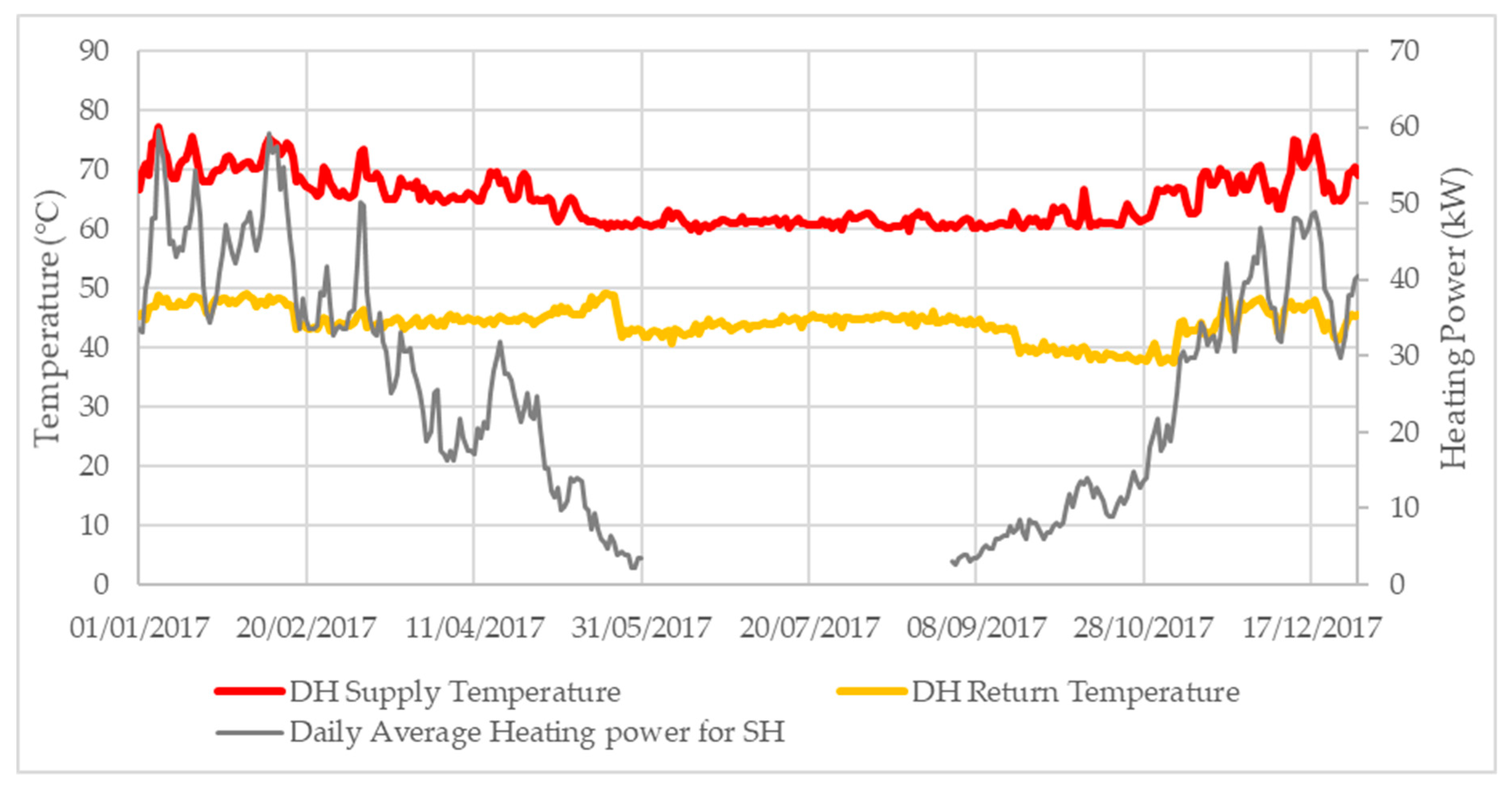
Figure 4.
Part load operation of the radiator system of the building case study in relation to the number of days during 2017, expressed as a duration curve.
Figure 4.
Part load operation of the radiator system of the building case study in relation to the number of days during 2017, expressed as a duration curve.
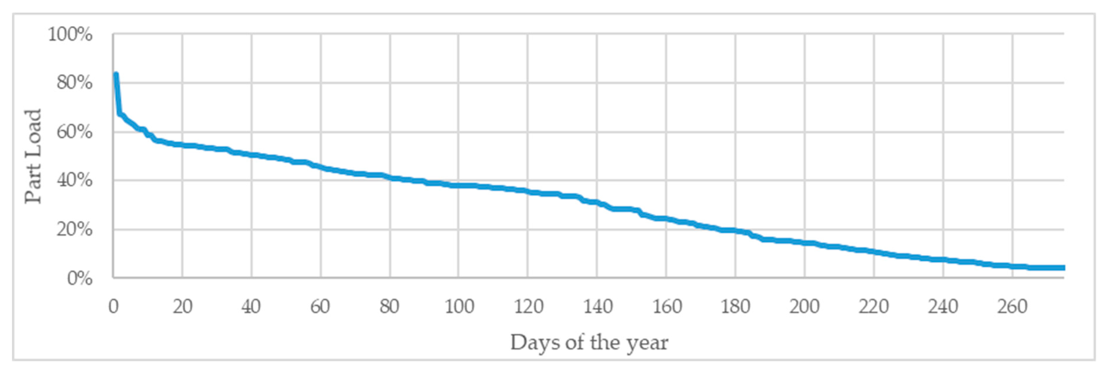
Figure 5.
Part load operation of the radiator system of the building case study in relation to the average daily ambient temperature for each day of 2017.
Figure 5.
Part load operation of the radiator system of the building case study in relation to the average daily ambient temperature for each day of 2017.

Figure 6.
The daily average DH supply and return temperature measured by the energy meter in the substation of the building case study, and the calculated expected DH return temperature due to the ideal operation of the radiator system during 2017.
Figure 6.
The daily average DH supply and return temperature measured by the energy meter in the substation of the building case study, and the calculated expected DH return temperature due to the ideal operation of the radiator system during 2017.
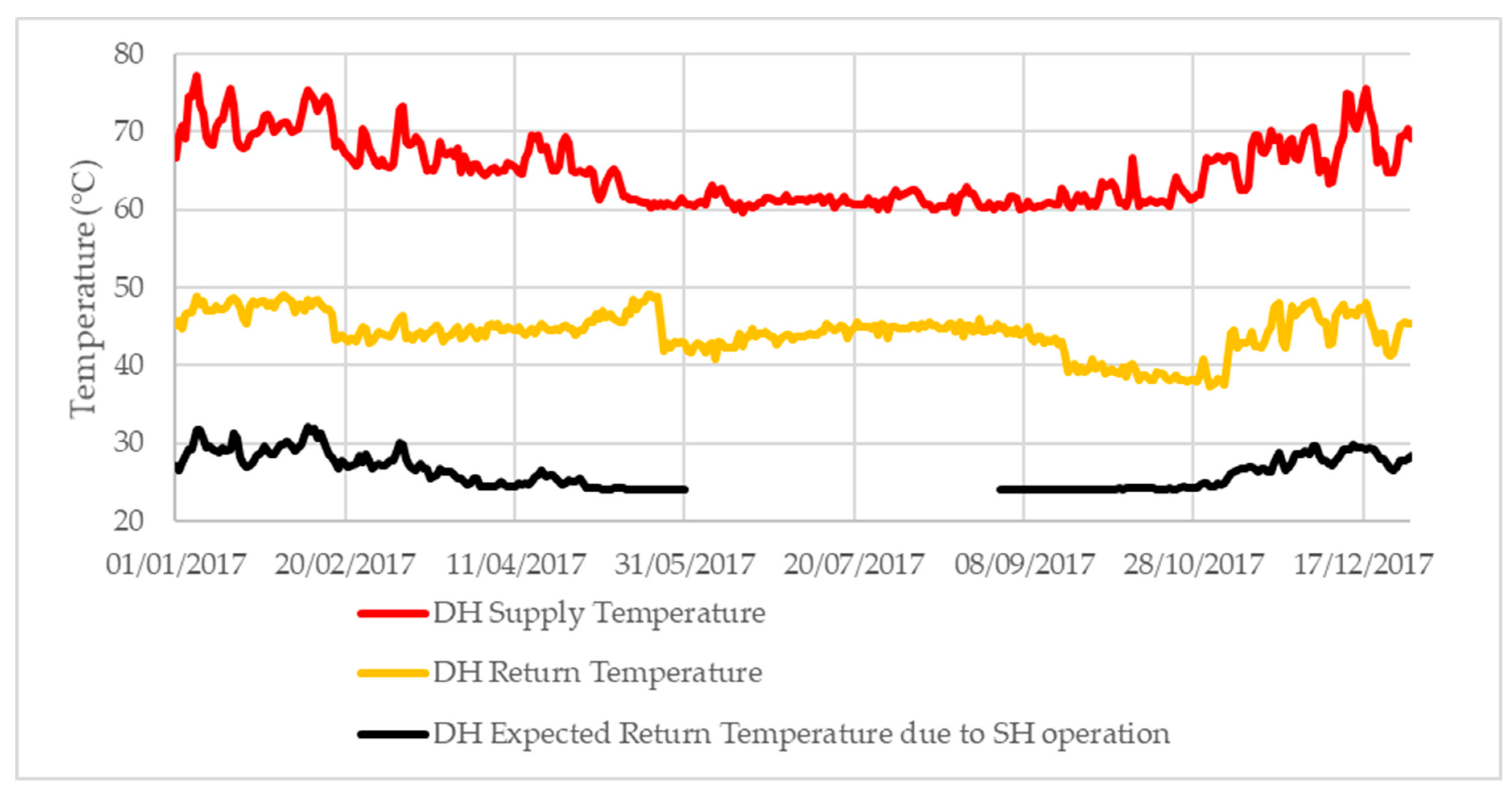
Figure 7.
The calculated optimal supply temperature and the return temperature results from the analysis for the operation without problematic thermostatic radiator valves (TRVs) and with one problematic TRV in each riser under low-flow system operation.
Figure 7.
The calculated optimal supply temperature and the return temperature results from the analysis for the operation without problematic thermostatic radiator valves (TRVs) and with one problematic TRV in each riser under low-flow system operation.

Figure 8.
The minimum pump pressure difference required and the system mass flow rate for the operation without problematic TRVs and with one problematic TRV in each riser under low-flow system operation.
Figure 8.
The minimum pump pressure difference required and the system mass flow rate for the operation without problematic TRVs and with one problematic TRV in each riser under low-flow system operation.
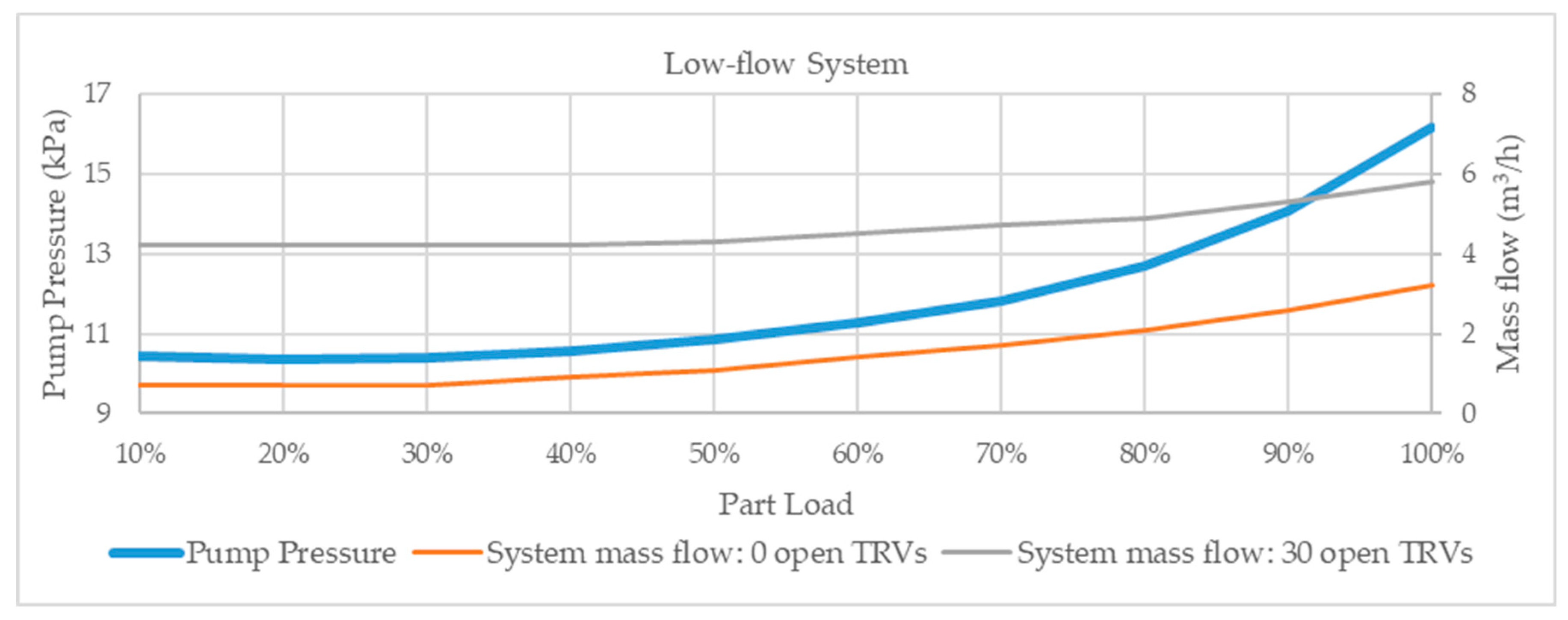
Figure 9.
The proposed weather compensation control of the supply temperature (orange line) under low flow system operation presented via a linear regression analysis.
Figure 9.
The proposed weather compensation control of the supply temperature (orange line) under low flow system operation presented via a linear regression analysis.
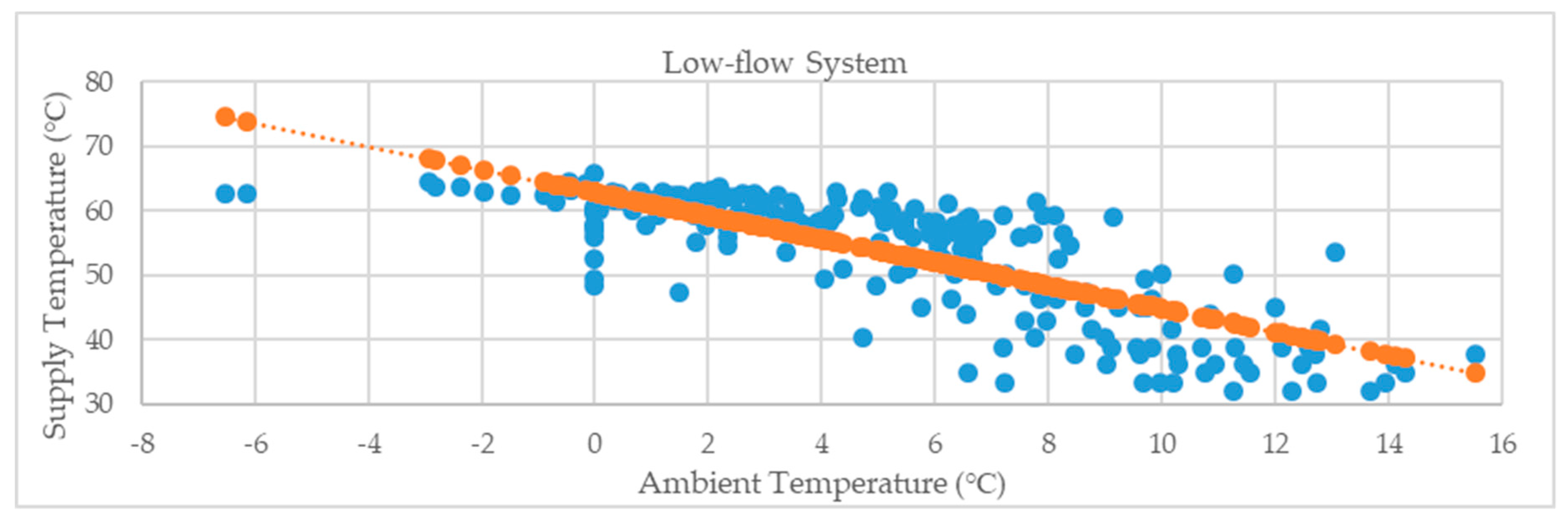
Figure 10.
The calculated optimal supply temperature and the return temperature results from the analysis for the operation without problematic TRVs and with one problematic TRV in each riser under high-flow system operation.
Figure 10.
The calculated optimal supply temperature and the return temperature results from the analysis for the operation without problematic TRVs and with one problematic TRV in each riser under high-flow system operation.

Figure 11.
The minimum pump pressure difference required and the system mass flow rate for the operation without problematic TRVs and with one problematic TRV in each riser under high-flow system operation.
Figure 11.
The minimum pump pressure difference required and the system mass flow rate for the operation without problematic TRVs and with one problematic TRV in each riser under high-flow system operation.
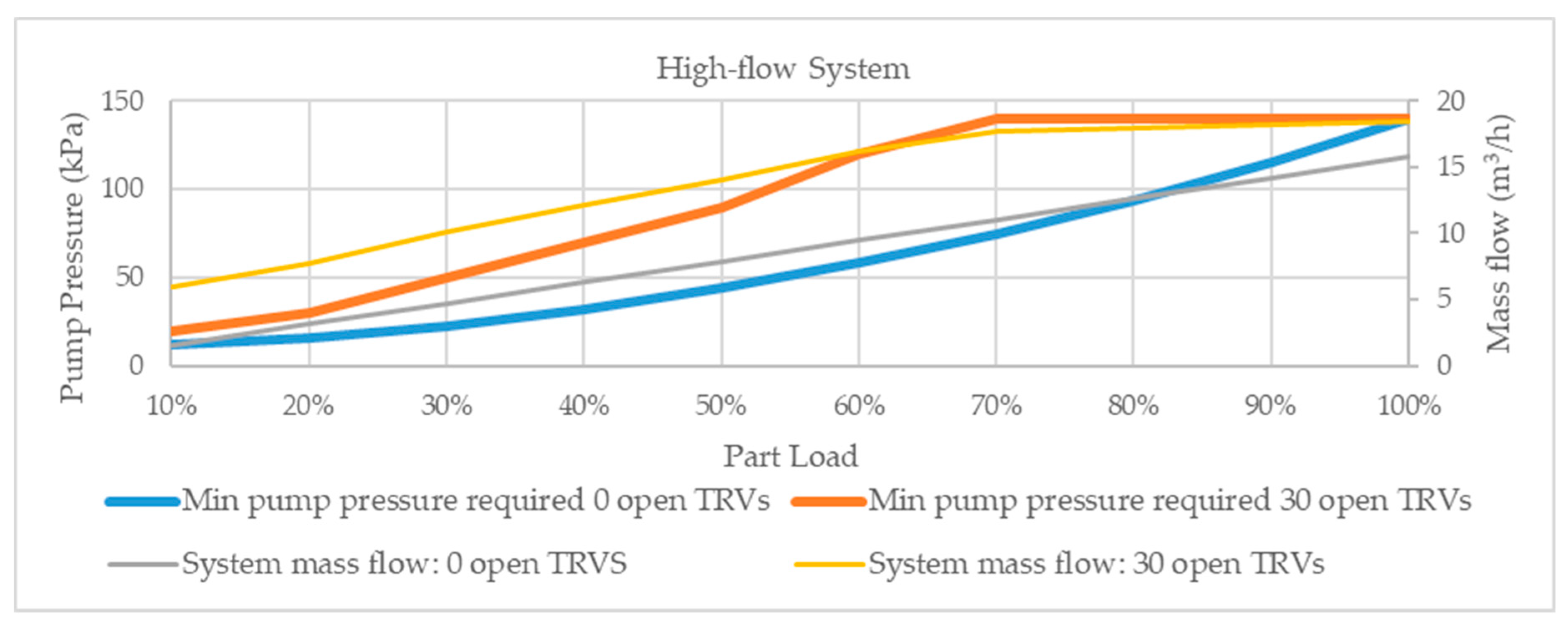
Figure 12.
The proposed weather compensation control of the supply temperature (orange line) under low flow system operation presented via a linear regression analysis.
Figure 12.
The proposed weather compensation control of the supply temperature (orange line) under low flow system operation presented via a linear regression analysis.
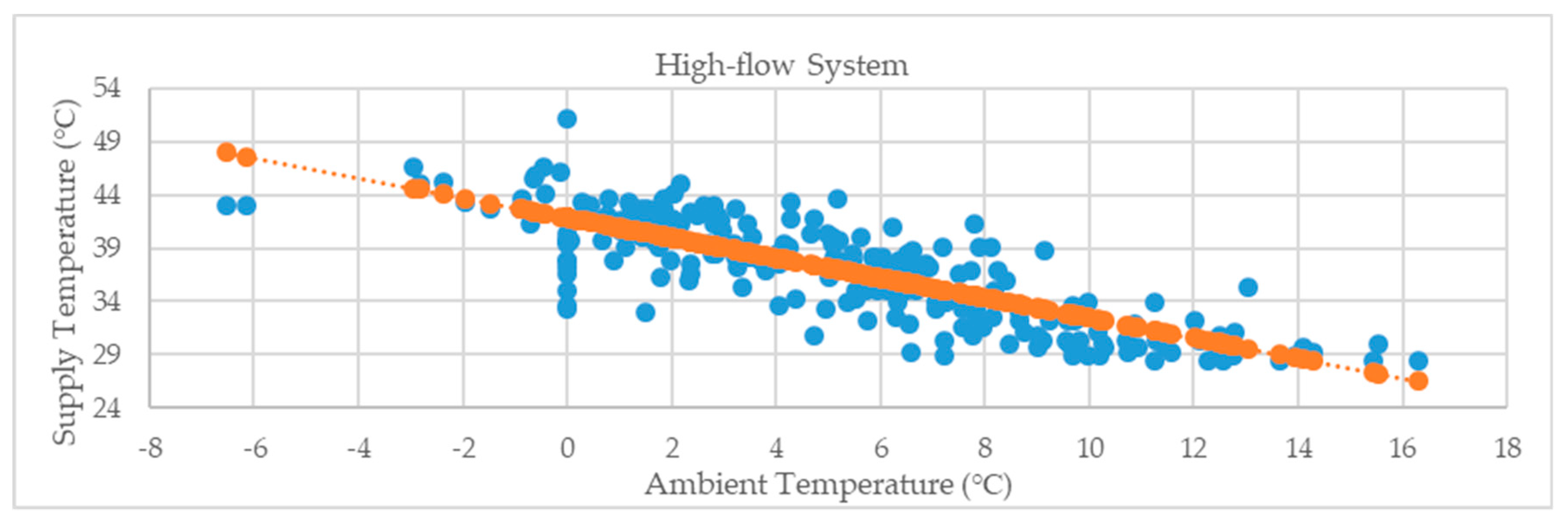
Figure 13.
(a) Thermocouple attached to the return pipe of a radiator element in an apartment; (b) Thermocouple attached to the return pipe and a riser in the basement before it is covered with insulation.
Figure 13.
(a) Thermocouple attached to the return pipe of a radiator element in an apartment; (b) Thermocouple attached to the return pipe and a riser in the basement before it is covered with insulation.
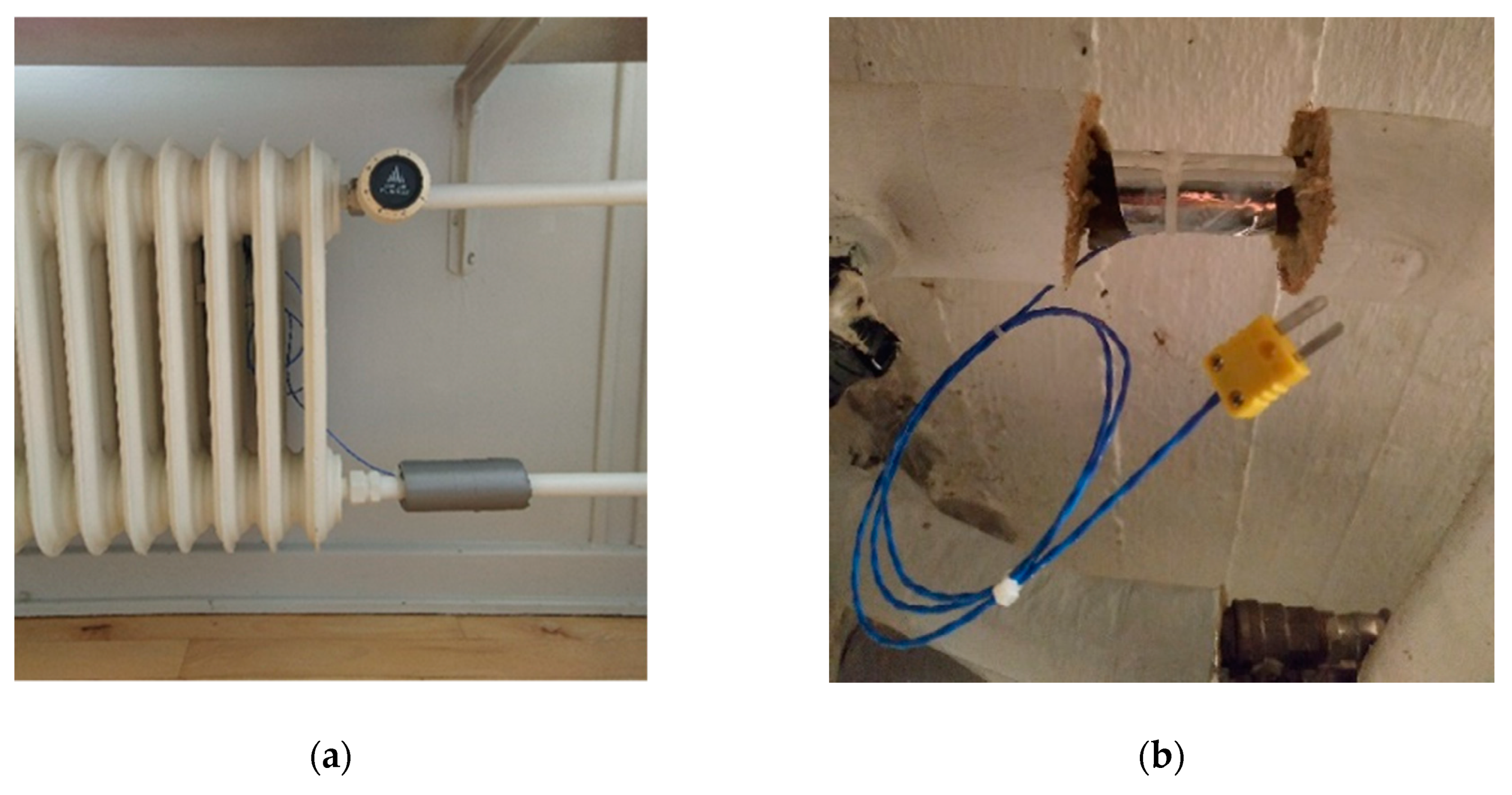
Figure 14.
Recording of the radiator system supply and return temperatures and the return temperature from several risers during the period between 16 November 2018 and 19 November 2018, before the implementation of the two suggested strategies.
Figure 14.
Recording of the radiator system supply and return temperatures and the return temperature from several risers during the period between 16 November 2018 and 19 November 2018, before the implementation of the two suggested strategies.

Figure 15.
Recording of the radiator system supply and return temperatures and the return temperature from all the radiators (Rad) of a specific apartment, located on the first floor at the west end of the building, during the period between 16 November 2018 and 19 November 2018, before the implementation of the two suggested strategies.

Figure 16.
Results of the first strategy based on the low-flow system operation tested on 26 November 2018 in the actual radiator system of the building case study in Viborg. The two curves represent the supply and the return temperature of the radiator system.
Figure 16.
Results of the first strategy based on the low-flow system operation tested on 26 November 2018 in the actual radiator system of the building case study in Viborg. The two curves represent the supply and the return temperature of the radiator system.
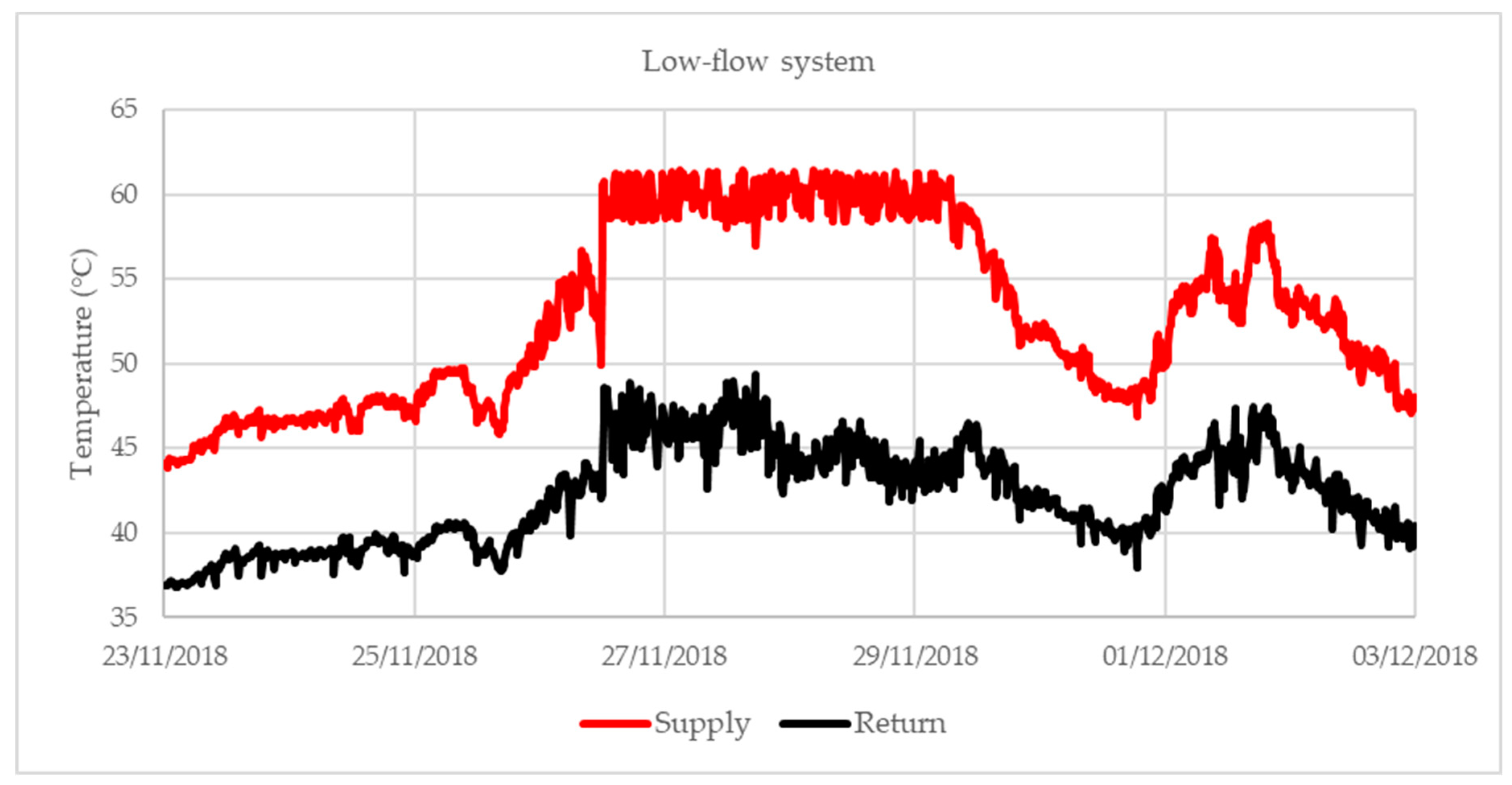
Figure 17.
Results of the second strategy based on the high-flow system operation tested under two steps on 11 February 2019 and 13 February 2019 in the actual radiator system of the building case study in Viborg. The two curves represent the supply and the return temperature of the radiator system.

Table 1.
Two different strategies were investigated to reduce the temperature of the radiator system of the building case study.
Table 1.
Two different strategies were investigated to reduce the temperature of the radiator system of the building case study.
| Strategy | Modeled | Tested |
|---|---|---|
| Low-flow system operation (by fixing errors and improving the use of TRVs as requirements) | ✓ | ✓ |
| High-flow system operation | ✓ | ✓ |
Table 2.
An overview of the calculation process performed by the thermal-hydraulic model in order to calculate the mass flow rate, the pressure difference of the pump and the return temperature of the radiator system under the ideal operation without problematic operation by the thermostatic radiator valves (TRVs).
| Step 1 | Selection of the supply temperature and the part load () conditions of the case. The design heat output () of each radiator in the system and the design supply and return temperatures are provided by the SH system operator and they are used as inputs for this calculation. |
| Step 2 | Calculation of the mass flow rate () and the pressure drop in every radiator, pipe section and the overall system for the reference case of the ideal operation of the system without errors, by using Equations (1)–(11). The minimum required pressure difference of the pump must be equal to the pressure drop of the system. |
Table 3.
An overview of the calculation process performed by the thermal-hydraulic model in order to recalculate the mass flow rate, the pressure difference of the pump and the return temperature of the radiator system under the case of one problematic TRV in every riser that causes uncontrolled flows in the system.
| Step 1 | Selection of one radiator in every riser with a fully open TRV that leads into an uncontrolled flow. |
| Step 2 | Selection of the minimum required pressure difference of the pump (), calculated under the ideal operation of the radiator system, as an input for the mass flow recalculation in the case of a fully open TRV in every riser. |
| Step 3 | Iterative recalculation of the mass flow rate () and the pressure drop in every radiator, by using Equations (1)–(12), due to the existence of the uncontrolled flows in the system (), calculated from Equation (12), for the constant pump pressure difference () selected in Step 2. |
| Step 4 | Evaluation of the optimal operation of the TRVs in the system, by accepting a minimum pressure drop in every functional TRV () higher than 5 kPa. |
| Step 5 | In case there are several TRVs with a pressure drop lower than 5 kPa, a higher pressure difference of the pump (), is selected as an input and the calculation in Step 3 is repeated until the condition in Step 4 is fulfilled. |
| Step 6 | When the condition in Step 4 is fulfilled, and the mass flow rate in every radiator () is recalculated due to the existence of uncontrolled flows (, the return temperature from every radiator and the overall return temperature of the system are calculated by using Equation (13). |
© 2019 by the authors. Licensee MDPI, Basel, Switzerland. This article is an open access article distributed under the terms and conditions of the Creative Commons Attribution (CC BY) license (http://creativecommons.org/licenses/by/4.0/).
Share and Cite
MDPI and ACS Style
Benakopoulos, T.; Salenbien, R.; Vanhoudt, D.; Svendsen, S. Improved Control of Radiator Heating Systems with Thermostatic Radiator Valves without Pre-Setting Function. Energies 2019, 12, 3215. https://doi.org/10.3390/en12173215
AMA Style
Benakopoulos T, Salenbien R, Vanhoudt D, Svendsen S. Improved Control of Radiator Heating Systems with Thermostatic Radiator Valves without Pre-Setting Function. Energies. 2019; 12(17):3215. https://doi.org/10.3390/en12173215
Chicago/Turabian StyleBenakopoulos, Theofanis, Robbe Salenbien, Dirk Vanhoudt, and Svend Svendsen. 2019. "Improved Control of Radiator Heating Systems with Thermostatic Radiator Valves without Pre-Setting Function" Energies 12, no. 17: 3215. https://doi.org/10.3390/en12173215
Note that from the first issue of 2016, this journal uses article numbers instead of page numbers. See further details here.