Quantitative Study of the Geometrical and Hydraulic Characteristics of a Single Rock Fracture


1
School of Mathematical Sciences, University of Electronic Science and Technology of China, Chengdu 611731, China
2
Institute of Petroleum Engineering, Heriot-Watt University, Edinburgh EH14 4AS, UK
3
School of Science, Institute for Artificial Intelligence, Southwest Petroleum University, Chengdu 611731, China
*
Author to whom correspondence should be addressed.
Energies 2019, 12(14), 2796; https://doi.org/10.3390/en12142796
Submission received: 10 June 2019
/
Revised: 11 July 2019
/
Accepted: 17 July 2019
/
Published: 20 July 2019
Abstract
:Three-dimensional images of fractured rocks can be acquired by an X-ray micro-CT scanning technique, which allows researchers to investigate the ‘true’ inner void structure of a natural fracture without destroying the core. The 3D fractures in images can be characterised by measuring morphological properties on both fracture apertures and its trend surface, like the medial surface, that reveals the undulation of fracture planes. In a previous paper, we have proposed a novel method to generate fracture models stochastically. Based on a large number of such fracture models, in this work a modified factor was proposed for improving the performance of the cubic law by incorporating the flow-dominant characteristics, including two parameters (aperture roughness and spatial correlation length) for fracture apertures and two (surface undulation coefficient and spatial correlation length) for fracture trend-surface. We assess and validate the modified cubic law by applying it to natural fractures in images that have varying apertures and extremely bended trend-surfaces, with the permeabilities calculated by a Lattice Boltzmann Method as ‘ground truths’.
1. Introduction
Natural fractures are common features in many rocks, occurring at various length scales and at different intensities. Understanding the fluid flow characteristics in natural fractured rock is of importance for petroleum reservoirs [1], geothermal energy development [2,3], nuclear waste disposal [4] and the geologic storage of carbon dioxide [5]. Since intact rocks are often low in permeability, and the fracture network forms the main channels of flow, the effective permeability of a fractured rock is dictated by the permeability of the fracture network, which consists of numerous individual fractures. Therefore, the fluid flow through a single fracture could form a basic building block for understanding the mechanical-hydraulic interactions of natural fractured rock, which has been extensively studied in recent years [6,7,8,9,10,11].
For steady laminar flow between smooth parallel plates, separated by a constant aperture, fracture transmissivity is proportional to the cubic power of fracture aperture, which is well known as the ‘cubic law’ [12]. However, the fractures in natural rocks have complex geometry and widely deviate from the parallel plate model. The cubic law should, therefore, be tuned to incorporate more factors that influence fluid flow [7,13,14].
Earlier theoretical works [15,16,17,18,19,20] usually use two-dimensional aperture fields to represent rough-walled fractures, and many efforts [15,17,19] have been made to assess the effect of variable fracture apertures on fluid flow. For example, Zimmerman [19] modified the cubic law with additional fracture roughness, which is defined as the ratio of aperture standard deviation over mean aperture. Tsang [17] and Moreno [15] analyzed the effect of aperture anisotropy on fracture fluid flow by taking account of the ratio of the spatial correlation length in different directions of aperture field. In addition, the fractal characteristics of fracture void space, consisting of variable apertures at different locations, was considered by Pyrak-Nolte [14] and it was subsequently incorporated into the study of fluid flow through rough-walled fractures. Although these literatures have thoroughly investigated the influence of fracture variable apertures on fluid flow in rough-walled fracture, using aperture field only to characterize a rough-walled fracture over-simplifies the fracture void space to a big extent. It assumes the void space to be perfectly planar, ignoring the natural undulation [20] or waviness in the alignment of the fracture voids. Therefore, in order to analyze the influence of rough fracture characteristics on fluid flow, it is constructive to consider the morphological features of the trend-surface (i.e., medial surface) of fracture profile, which realistically describes the undulation of fracture planes. Similarly, the morphological analysis can also be applied to the pores of rock matrix [21,22].
Advances in imaging technology make it possible to obtain 3D images of fractured rocks. One example of the imaging technology is X-ray computed tomography (CT) [1,23,24,25,26] that can detect the inner structure of nontransparent objects without destroying rock samples. The principle of CT is that different rock components (e.g., minerals, pores, fracture voids, fluids) have different densities, resulting in different X-ray absorption coefficients, which are then converted into different gray values in resultant 2D images that can be used to distinguish the solid and pore space (fracture void) [25] in this work. Simply, they are both precise and direct methods for developing digital fractured rocks, providing a basis for quantitating the geometric features of the fracture void space [27,28].
With 3D digital rocks, there are two major numerical approaches to simulate single- and multi-phase flow processes: direct simulation and pore-network modelling (PNM) [29,30,31,32,33,34,35,36]. Examples of the direct simulation method includes finite difference/element/volume methods [37,38,39] and the Lattice Boltzmann method (LBM) [40,41,42,43,44,45]. However, for the finite difference/element/volume methods, it is a challenging and time consuming issue to deal with the expensive mesh generation and irregular geometries. With regards to those limitations, the LBM has been widely applied to simulate the flow behaviors in 3D digital rock. The advantages of the LBM include simple algorithms, efficient parallelization, and flexibility in implementing complex flow geometries, which makes the LBM profoundly powerful in the simulation of single- and multi-phase fluid flow through porous media. As for the PNM, it is designed to simulate fluid flow on a simplified structure described by a network of pore bodies (nodes) connected by pore throats (bonds). Each network element (i.e., node or bond) is associated with a regular (e.g., a star, triangle, square, or circle) cross section and assigned with a set of geometrical properties (e.g., radii, volume, shape factor, and length), which makes the numerical simulation based on PNM more complex than LBM. Therefore, in this work, we use the LBM simulations of fluid transport with X-ray topographies to estimate fracture permeability.
The objective of this work is to quantitatively determine the collective effects of both fracture apertures and the trend-surfaces on fluid flow in single fractures. To address this, their characteristic parameters are firstly extracted from digital fractured rocks. Fracture structural models are then generated with various parameters about fracture apertures and trend-surfaces. Subsequently, the LBM is applied to simulate fracture flows for predicting fracture permeability, and further a modified version of the cubic law, which incorporates geometric fracture undulation, is proposed and validated by applying it to natural fractured cropped out from 3D μCT images.
2. Methodology
2.1. Fracture Morphology
2.1.1. Natural Fracture in CT Images
A 3D digitized rock, which reveals the pore structure in the rock matrix and fracture opening/void, is made up of a series of 2D images which are obtained by X-ray computed tomography (CT). Figure 1 shows an example of a stack of cross-sectional slice CT images of a shale core, which includes fracture structure (e.g., red box in Figure 1a) and were provided by iRock Technologies (http://www.irocktech.cn/). These 1024 successive 2D shale images in Figure 1a were aligned and stacked to form a 3D image (see Figure 1b), with 1024 × 1024 × 1024 voxels and 12.9 μm/voxel.
2.1.2. Fracture Characterization
Prior to discussing how to represent the fracture geometries, we must first introduce the approaches in measuring fracture morphological properties regarding fracture apertures and fracture trend-surface.
Figure 2a shows a 2D slice of a cropped grayscale sub-image of 300 × 300 × 100 voxels from the shale CT-image (red box) shown in Figure 1a. A binary image in Figure 2b, consisting of only solid and fracture void, can be obtained by segmenting the grayscale image using the threshold segmentation method [46]. Thus the fracture volume fraction (or porosity) of the 3D shale sub-image can be calculated as 9%, which is the ratio between the fracture void and rock volume. Meanwhile, based on the binary image, three structural components of a fracture, as shown in Figure 2c, can be extracted by the edge detection operator [46]. Defining the plane of height Z = 0 as a reference, the spatial relative positions of the upper and lower fracture-wall surfaces at a coordinate ζ = (x, y) on the plane can be determined, denoted by zU(ζ) and zL(ζ), or zU and zL for short. The fracture local aperture b(ζ) at a point ζ, which is described as the length of the two-way arrows in Figure 2c, can be simply calculated by:
It is worth noting that if the fracture profile in the rock extends horizontally at the XY plane, the fracture aperture can be approximated by the height difference between the upper and lower fracture surfaces, as referred to in [8]. If the fracture is placed non-horizontally at the XY plane, the fracture aperture, i.e., the shortest distance between fracture two surfaces, can be calculated with the help of the fracture medial surface, which the calculation details can be referred to [47,48]. In our work, all fractures are assumed horizontal extending at the XY plane, and the height difference between the upper and lower fracture surfaces is choose as the fracture aperture (see Equation (1)).
The red curve in Figure 2c was obtained by smoothing the mid-surface, zM (see Equation (2)), using the image filter operator [46], and denoted as zT (see Equation (3)). The heights of the trend-surface quantifies the spatial fluctuation of a fracture.
where g(.) is a moving average smoothing operator.
Therefore, fracture void space can be equivalently characterized by two elements: apertures and trend-surface.
With respect to fracture apertures that vary in a range, mean aperture, μb, and standard deviation, σb, can be estimated from the aperture density distribution, and then we have the ratio of the standard deviation and the mean aperture, σb/μb, to quantify fracture roughness [19]. In addition, the spatial correlation between apertures at different locations can be described by a scalar, i.e., aperture spatial correlation length, which can be described by the semi-variogram function [49]. Let φ be a stochastic variable defined on a discrete domain Ω ⊂ R and h = (x, y) be a (direction) vector, the semi-variogram γφ(h) between variables φ(ζ) and φ(ζ + h) is defined as:
where E[] denotes the mathematical expectations, ζ is evaluated over all positions in Ω, and the variable φ can be the fracture apertures (Equation (1)) or surface heights (Equation (3)). Note that the closer two locations (i.e., ζ and ζ + h) are, the smaller the semi-variogram value becomes.
Similarly, for the fracture trend surface (Figure 2d), zT, the corresponding standard deviation, σT, and spatial correlation length, λT, can be estimated using the height density distribution of zT and the surface semi-variogram, respectively. It is noticed that σT can also be considered as a coefficient to characterize fracture undulation, which reveals the undulation strength on fracture plane.
In summary, in this work the key properties influencing fracture morphology are μb, σb, λb for fracture apertures (fields) and σT, λT for fracture trend surface.
2.2. Modified Cubic Law
A single fracture is usually modelled by two smooth parallel plates separated by a constant width (i.e., aperture), , which is approximated by the arithmetic average of apertures for a rough-walled fracture [50], i.e., ≈ μb. Many researchers [13,20,43] have shown that for the steady state, isothermal, laminar flow between parallel plates, the absolute permeability, KCL, of a fracture is a function of fracture spacing (i.e., aperture), and estimated by the following equation (i.e., the cubic law):
However, neglecting the morphological complexity of the void/opening space of natural fractures results in the failure using the cubic law to predict the permeability accurately due to –that in Equation (5) is not able to sufficiently represent aperture variation, thus commonly a modified factor [43], f is introduced in Equation (5) to take into account of the fracture complex morphology as:
To determine f we can use the following formula:
where K is assumed to be true permeability, which is actually approximated by the LBM calculation in this work.
2.3. Fracture Modelling
In this work, each model of a rough-walled fracture is generated by combining two random two-dimensional fields into a fracture aperture map b(x, y) and a trend surface zT(x, y). Assuming that these two fields are defined on the XY plane, and both the aperture field and the trend surface are suggested to be normally distributed and are spatially correlated. In our previous work [51], an image mean-filter method has been proposed to generate such fields independently and then to assembly into a 3D fracture, as shown in Figure 3, subject to five pre-measured morphological parameters, μb, σb2, λb, σT2 and λT. Note that the actual position of the trend surface has no impact on the aperture distribution of a resultant fracture, so μT can be randomly chosen in modelling.
The method includes three major steps: (1) sampling data from a uniform distribution and then filtering the data with a pre-defined mean mask to obtain a trend surface field that has the required distribution and the pre-specified correlated feature, associated with two input parameters: σT2 and λT. The data field is used as fracture trend surface, illustrated in Figure 3, denoted as zT; (2) Generating two more fields independently in the exact same means as the first step for the two fracture walls with three specified aperture parameters: μb/2, σb2/2 and λb. The resulting two data fields, denoted as dU and dL, are the relative heights in relation to the trend surface in two opposite directions, as demonstrated in Figure 3; (3) Positing the two wall fields above or below the trend surface in horizontal direction into an upper surface, zT + dU, and a lower surface, zT − dL, respectively. Let b be dU + dL, i.e., a local aperture at a location on XY plane. Over the whole XY plane the resultant fracture is determined by five statistical parameters: mean aperture μb, aperture variance σb2, aperture correlation length λb, trend surface variance σT2 and trend surface correlation length λT.
As an example, Figure 4 shows three 3D fracture models generated using our mean-filter method with five input morphological parameters. Note that the fracture shapes are different from each other even though with the same input morphological parameters, which gives a certain amount of freedom in fracture shape but capture the controlling morphology.
2.4. Fracture Permeability Calculation
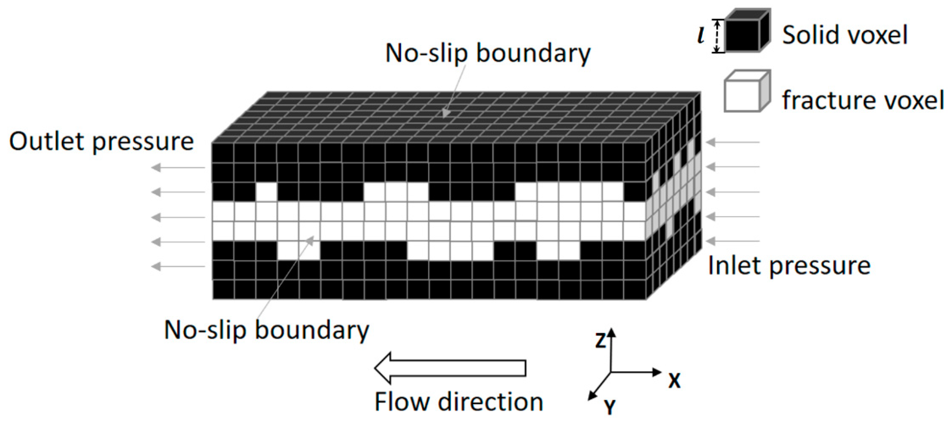
On 3D fracture models, single-phase can be simulated using Palabos [52], Lattice-Botlzmann method (LBM) software, which is an open-source code for computational fluid dynamics. As the LBM is highly flexible and parallel implemented, it can handle a wide variety of fluid dynamics problems [40,41,42,43]. In this study, the Palabos LBM software is utilized to compute absolute permeabilities only for a large number of fracture models under an assumption of the bounce-back boundary condition for fracture walls. The fracture walls, as shown in Figure 5, parallel to the flow direction, are padded to eliminate the need for periodic boundaries. The standard Bhatnagar-Gross-Krook (BGK) collision operator is applied with a D3Q19 model. Initially, the fluid macroscopic density in the inlet is set to one and the fluid velocity is set to zero everywhere and fluid movement is induced by maintaining a constant pressure gradient between the inlet and outlet, which is set as 5 × 10⁻⁵ Pa in addition to a lattice viscosity of 0.167 for all models. Steady state will be reached when the standard deviation of the average energy, measured over a fixed number of time steps, fall below a given threshold value (e.g., 3000 time steps, or a threshold value of 10−4). Steady-state results of the model are then analyzed to simulate absolute permeability. Given the velocity distribution throughout a 3D domain, the “true” permeability K in Equations (6) and (7) of a fractured rock model is calculated by the Darcy’s law:
where dP/dx is the pressure gradient along X-direction, μ is the fluid viscosity, and U is the average velocity through a cross-section.
Actually, the fractured rock permeability, calculated by Palabos code, is in dimensionless lattice (or image voxel) units and marked as Kl hereafter. This value is easily converted to physical units Kr by Equation (9) [45]:
where l is the physical side-length of a voxel, as shown in Figure 5.
Considering that the rock models studied in our work contain a single fracture only, the fracture permeability Kf is computed instead by [53]:
where φ is the volume fraction of fracture void in the rock models.
Since the computation of permeability using the LBM has been evaluated as a reliable approximation to the real permeability, which have been validated by comparing simulated results with experimental data in reference [45]. In our work we also denote the permeability calculated by the LBM as KLB, i.e., Kf = KLB.
3. Results and Discussion
3.1. Robustness of Fracture Modelling
Regarding the fracture models generated by our mean-filter method, the fracture shapes demonstrate a certain amount of randomness between individual models for the same input morphological parameters, i.e., μb, σb, λb, σT2, λT, see Figure 4. Further, it is worthwhile investigating the robustness of these models in terms of their permeabilities before we carry out studying the effect of fracture morphology on single-phase flow. In other words, we need to assess how robust the fracture models are that have the same input parameters on fracture permeability rather than fracture shapes. For instance, μb = 8.7 voxels, σb2 = 3, λb = 6 voxels, σT2 = 61, and λT = 200 voxels are the five morphological properties measured from the fracture illustrated in Figure 2, and can be used as input parameters to generate any number of fracture models (realizations). Figure 6 shows the relative errors in the LBM permeability between such 15 realizations and a nature fracture in Figure 2, in which the relative error ε, is defined as |k − ko|/ko, where ko and k are two permeabilities of the natural fracture and one of the realizations, respectively. It is evident that different fracture realizations for the same input parameters differ only within a narrow range (ε < 15%), which indicates that our modelling method captures the essential morphology that dominates single-phase flow. Although the numerical fractures are not identical entirely to the actual fracture in shape, their corresponding permeability is sufficiently close, therefore the method is robust in this sense.
3.2. Influence of Fracture Trend Surface
The morphological parameters (i.e., σT2, λT) are introduced in Section 2 to characterize the fracture trend surface. In order to study the impact of the trend surface on petro-physical properties (especially the permeability) associated with fractures, three groups of single fracture models of 300 × 300 × 100 voxels are generated using the algorithm briefly introduced in Section 2.3, within each group every fracture has the same mean aperture: 5, 9, 13 (in voxels) for group 1, 2, 3, respectively. In each group, there are 25 fracture models which generated by pairing these two sets of trend surface parameters: σT2 = 10, 50, 90, 130, 170; λT = 120, 160, 200, 240, 280 (in voxels), meanwhile, to eliminate the influence of fracture aperture field, we fix σb2 = 0 and λb = ∞ (i.e., constant apertures at everywhere). Only six fracture models are shown in Figure 7 to demonstrate the different morphology with respect to σT2 and λT. Using the LBM, 25 fracture permeabilities can be calculated for each group, followed by calculating 25 modified factors (fT) according to Equation (7).
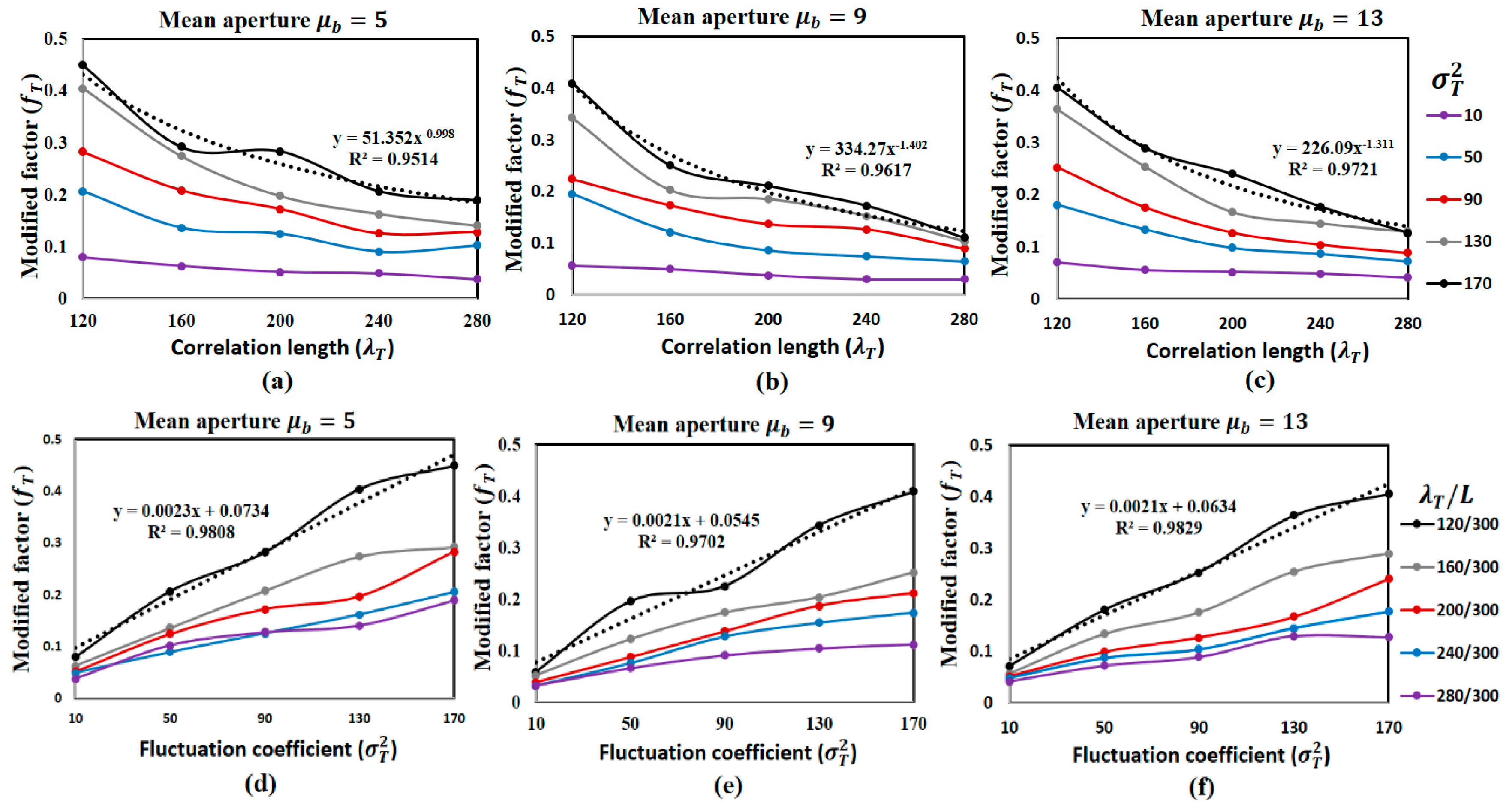
With the correlation lengths (λT) and the undulation coefficients (σT2) about the fracture trend surfaces in each group, we relate the corresponding modified factors, as shown in Figure 8a,d, Figure 8b,e, and Figure 8c,f for group 1, 2 and 3 of mean apertures of 5, 9 and 13 voxels, respectively. It is observed that with fixed undulation coefficient and mean apertures, the modified factor is a power-law function of the correlation length as the dotted curves shown in Figure 8a–c. As the longer the correlation length is, the gentler the bending of the trend surface is, consequently the fracture wall is smoother and therefore the modified factor is smaller. This means that the flow path in the fracture is shorter, thereby increasing the fracture permeability. However, when the undulation coefficient decreases, the fracture models are more plate-like. In this circumstance, for instance σT2 = 10 (see Figure 8a–c), changing the correlation length of the fracture trend surface hardly affects the fluid flow path in the fracture, thus the modified factor tends to be zero.
With fixed correlation lengths and mean apertures, Figure 8d–f reveals the relationship between the modified factor and the undulation coefficient for the three groups. It can be seen that when correlation length remains constant, the modified factor increases linearly as the undulation coefficient increases. The undulation coefficient reflects fracture tortuosity, and so the greater the tortuosity is, the longer the flow path is, therefore the fracture permeability decreases. In addition, in Figure 8d, we found that there are some crosses existing. In Figure 8d, the curves with different colors represent different correlation lengths (λT) of trend surface, and the distance between curves decreases with the increase of correlation length (λT). When the correlation length is 240 (blue curve) and 280 (purple curve) in Figure 8d, the two curves are closest to each other. Therefore, the crossing of curves in Figure 8d may be caused by numerical errors.
Depicting a triple of fT, σT2 and (dimensionless) λT/L as a dot in Figure 9 for every fracture in the three groups, a 3D surface can be fitted by the least square fitting method. The fitted function (Equation (11), R2 = 0.86) for the surface can be obtained as:
This reflects that the modified factor increases linearly with the undulation coefficient, and decreases with the correlation length as a power function. In addition, we found that the power in Equation (11) is −1.39 and the power of the dotted lines in Figure 8b,c are closed to −1.39, while the value in Figure 8a is −0.99 and quite larger than −1.39. The reason of this phenomenon is that the dotted lines in Figure 8a–c are the optimal fitting of the power formula for the black solid lines. Although, the power in Figure 8a differs greatly from that in Figure 8b,c, the coefficient of power function in Figure 8a is much smaller than that in Figure 8b,c, which make up for the difference between the formulas in Figure 8a–c.
3.3. Influence of Fracture Aperture Variation
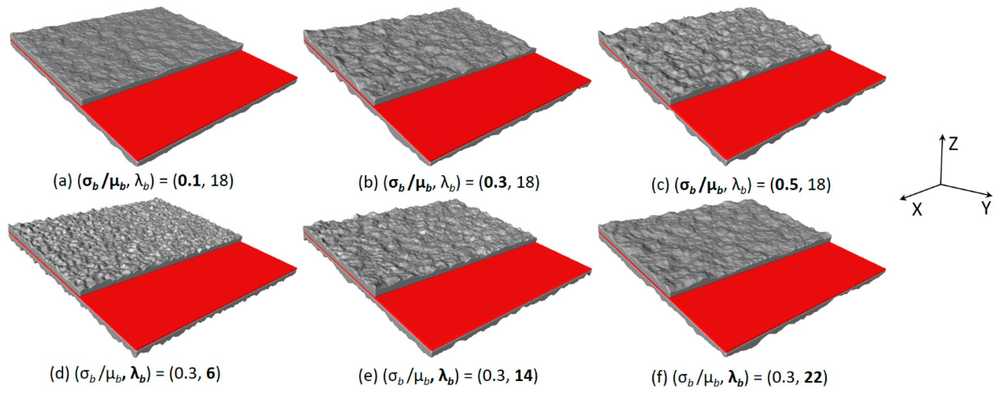
Regarding to the morphological parameters (i.e., μb, σb, λb) for fracture apertures, similarly, three groups of fracture models of 300 × 300 × 100 voxels are also generated, having the mean aperture (μb) of 5, 9, 13 voxels for Group 1, 2 and 3, respectively. Differently the two trend surface parameters are fixed as σT2 = 0 and λT = ∞ to eliminate the impact of trend surfaces, while only the aperture smoothness and aperture correlation length are allowed to pair between σb/μb = 0.1, 0.2, 0.3, 0.4, 0.5, and λb = 6, 10, 14, 18, 22. As a result we have 25 fracture models in each group and 75 models in total, of which six fracture models are shown in Figure 10.
Figure 11a–c presents the relationship between the modified factor (Equation (7)) and aperture correlation length based on the generated fracture models in Group 1, 2 and 3, respectively. It is evident that the modified factor seems to be a power function of the correlation length when σb/μb is constant. This is because the longer the correlation length the stronger the continuity between local apertures. Consequently, the obstruction of fluid flow in the fracture is reduced and increasing the degree of flow movability.
Similarly, Figure 11d–f describes the relationship between the modified factor and aperture roughness when λb/L is constant. It can be concluded that under the same correlation length of aperture fields, the modified factor is linearly related with the aperture roughness. This is because the roughness determines the range of variation between local apertures. The larger the roughness the greater the undulation of apertures, which hinder fluid flow and so reduces the fracture permeability.
Depicting a triple of fb, σb/μb and λb/L as a dot in Figure 12 for every fracture in the three groups, a 3D surface can be fitted in the same way as above. The fitted function (R2 = 0.83) for the surfaces can be obtained as:
It shows that the modified factor is a linear function of aperture roughness, but a power function of the aperture correlation length.
3.4. Accumulated Influence of Fracture Morphology
Quantitative studies on how the variation in both fracture trend surface and fracture apertures effects the modified factor in the cubic law (Equation (6)) have been discussed above separately. The accumulated influence may be complicated and has no systematical way to study, however it is necessary to investigate the function relationship between the two factors, fT and fb, and the total modified factor f in Equation (7).
In the same way as described in above sections, three groups of fracture models of 300 × 300 × 100 voxels can be generated, within each group every fracture has the same mean aperture: 5, 9, or 13 (in voxels), respectively. In each group there are 50 fracture models, of which 25 fracture models were generated by altering the trend surface parameters: σT2 = 10, 50, 90, 130, 170, λT = 120, 160, 200, 240, 280, where the fracture aperture parameters were fixed as σb/μb = 0.5 and λb = 22; meanwhile the other 25 fracture models were generated by changing the aperture parameters: σb/μb = 0.1, 0.2, 0.3, 0.4, 0.5; λb = 6, 10, 14, 18, 22, but the fracture trend surface parameters were fixed as σT2 = 100 and λT = 120. As a result, we have 150 models in total, of which eight fracture cross-sections are shown in Figure 13 to demonstrate the different morphology with respect to (σT2, λT) or (σb/μb, λb). Using the LBM, we have 150 fracture permeabilities and the corresponding modified factors f, furthermore we have the corresponding fT and fb for each fracture model according to Equation (11) and Equation (12).
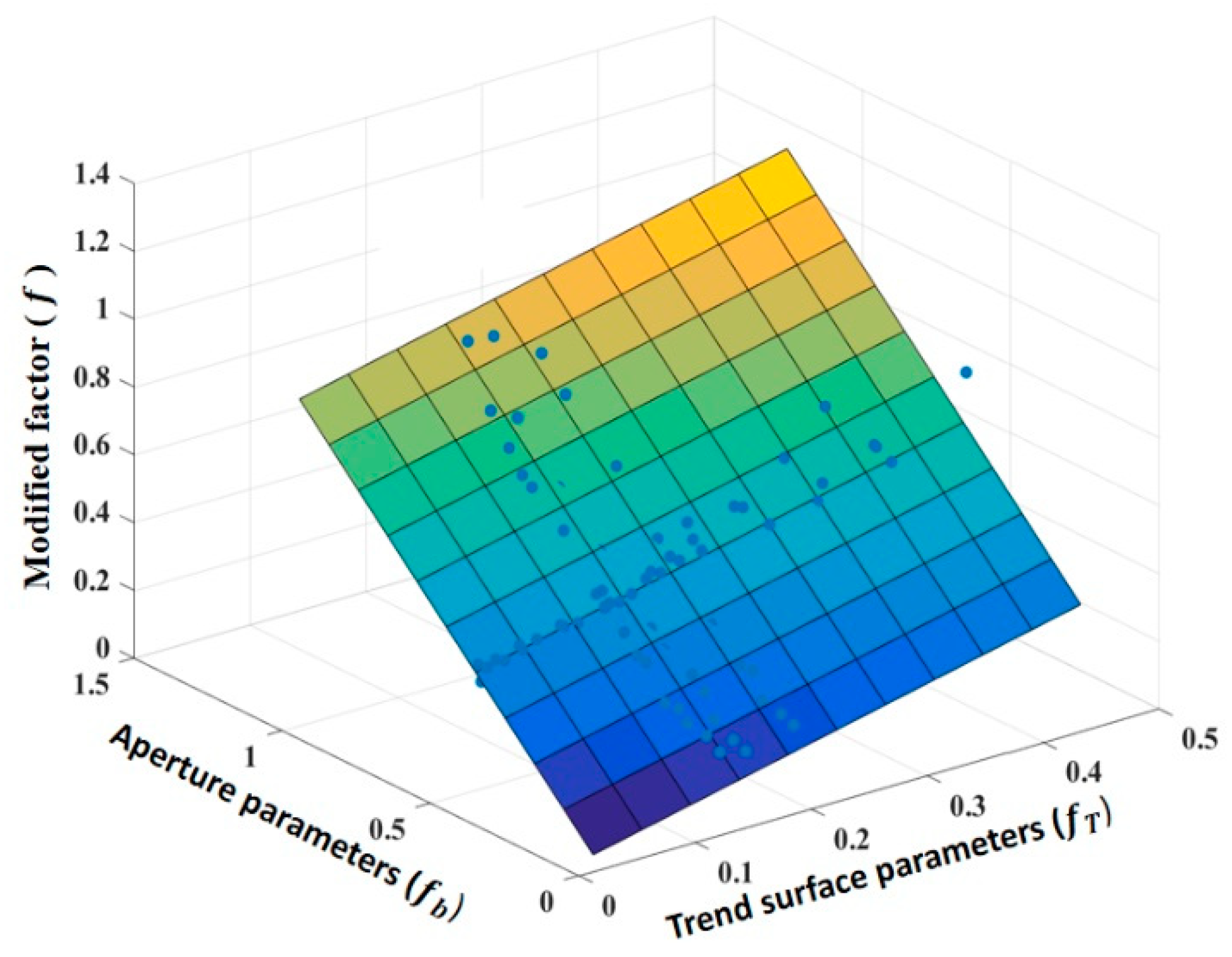
Depicting a triple of f, fT and fb as a dot in Figure 14 for every fracture in the three groups, a 3D surface can be fitted for the data by the least square fitting method. The corresponding function (R2 = 0.85) for the fitted surface can be estimated by:
It is shown that the slope of the modified factor caused by the aperture parameters (fb) is larger than the slope of the trend surface parameters (fT) because more weight is assigned, which indicates that the morphological characteristics of fractures described by (μb, σb and λb) are the predominant factor that effect the fluid flow more significantly. Therefore, the modified factor in Equation (13) is used to refine the cubic law as given in Equation (6). Next, we will use natural fractures in CT images to validate the calculation of the modified factor by Equation (13).
4. Verification with Natural Fractures
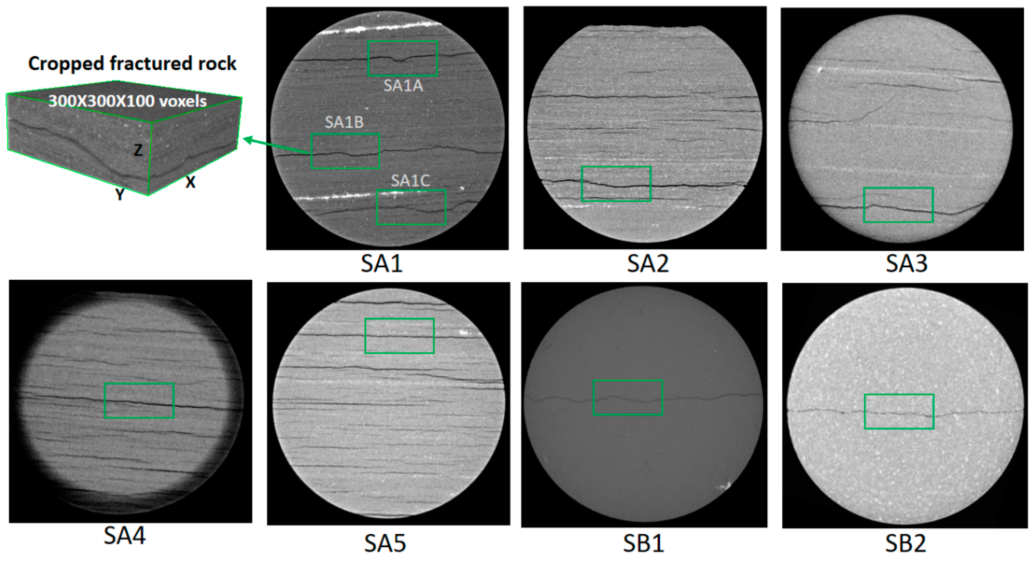
Figure 15 shows seven slice images of a CT image acquired by scanning seven fractured rock cores, all the images have the same dimensions of 10243 voxels, and the voxel resolution is assumed to be 1 μm/voxel without loss of generality. The first five are shales and the last two are sandstones. Instead of using the whole original images, a small sub-image (see Figure 15 is cropped out from each CT image to reveal a natural fracture. All fractures in Figure 15 can be considered to be horizontally placed. Using the measurement method described in Section 2.1.2, we can measure all the geometrical parameters of the trend surface and fracture aperture fields in the CT images, as listed in Table 1. Three types of fracture permeabilities for each fracture sample were calculated using LBM, cubic law, and our modified cubic law, KLB, Kcl, Kmcl, respectively. Let KLB be the permeability calculated by the LBM, and Kcl and Kmcl be the permeabilities estimated by the original cubic law of Equation (6) and our modified cubic law (Equations (7) and (13)), respectively. The relative errors are εcl = (Kcl − KLB)/KLB and εmcl = (Kmcl − KLB)/KLB. Note that from the table that the relative errors calculated by the modified cubic law are far less than that of the original cubic law: Most of them, remain below 20%, and the average relative error is ~8.57%, which are acceptable in practical applications. Therefore, based on the combination of fracture trend surface and variable apertures, the modified cubic law ((Equations (7) and (13)) proposed in this work effectively calculates the permeability of rough fractures, greatly reducing the computational complexity.
5. Conclusions
Advances in 3D imaging technology allow the fracture structure in fractured rocks to be revealed truly and faithfully without destroying the core. In this study, the rough-walled fracture was investigated by combining fracture variable apertures and the fracture trend surface topography, which quantifies undulation about the fracture undulation. Using the computer laboratory, the geometric characteristics of variable aperture and fracture trend surface were quantitatively represented, in which the aperture roughness and aperture correlation length used to describe variable apertures, and the trend surface fluctuation coefficient and the trend surface correlation length used to represent the fracture trend surface. In addition, the influences of these representation parameters on the fracture permeability of fluid flow through rough-walled fracture were investigated. Lastly, a corrector factor is proposed for improving the performance of the cubic law by incorporating the characteristic parameters of fracture trend surface and variable apertures. For all the 3D digital fracture samples present in this work, the modified cubic law was determined to be an acceptable approximation to the numerical simulation (LBM).
Because single fracture is the basic element of fracture network, the methodology has the potential application in characterizing the geometric structure of fracture network in which the interaction between fractures can be take into account. Meanwhile, the flow properties of the fracture network can be evaluated by the modified cubic law proposed in this work. These tasks will be processed in our next work. Apart from this extension, the applicability of our methods proposed in this work may be limited within a narrow range of length-scale (fracture opening in μm, mm or cm, plus the model dimensions), we will explore both in the near future, however the inertial effect and surface contact are neglected in our work and will be investigated in the future.
Author Contributions
Each author has made contribution to the present paper. Conceptualization, X.L. and Z.J.; methodology, X.L.; software, X.L.; validation, X.L.; formal analysis, X.L.; investigation, X.L.; data curation, Z.J.; writing—original draft preparation, X.L.; writing—review and editing, Z.J., C.M.; visualization, X.L.; funding acquisition, Z.J.
Funding
This research was funded by NSFGC, grant number 61572007.
Conflicts of Interest
The authors declare no conflict of interest.
References
- Karpyn, Z.T.; Grader, A.S.; Halleck, P.M. Visualization of fluid occupancy in a rough fracture using micro-tomography. J. Colloid Interface Sci. 2007, 307, 181–187. [Google Scholar] [CrossRef] [PubMed]
- Rutqvist, J.; Wu, Y.S.; Tsang, C.F.; Bodvarsson, G. A modeling approach for analysis of coupled multiphase fluid flow, heat transfer, and deformation in fractured porous rock. Int. J. Rock Mech. Min. Sci. 2002, 39, 429–442. [Google Scholar] [CrossRef]
- Hu, R.; Liu, Q.; Xing, Y. Case study of heat transfer during artificial ground freezing with groundwater flow. Water 2018, 10, 1322. [Google Scholar] [CrossRef]
- Tsang, C.F.; Bernier, F.; Davies, C. Geohydromechanical processes in the excavation damaged zone in crystalline rock, rock salt, and indurated and plastic clays - in the context of radioactive waste disposal. Int. J. Rock Mech. Min. Sci. 2005, 42, 109–125. [Google Scholar] [CrossRef]
- Liu, S.; Sang, S.; Pan, Z.; Tian, Z.; Yang, H.; Hu, Q.; Sang, G.; Qiao, M.; Liu, H.; Jia, J. Study of characteristics and formation stages of macroscopic natural fractures in coal seam #3 for cbm development in the east qinnan block, southern quishui basin, china. J. Nat. Gas Sci. Eng. 2016, 34, 1321–1332. [Google Scholar] [CrossRef]
- Wang, L.; Cardenas, M.B. Development of an empirical model relating permeability and specific stiffness for rough fractures from numerical deformation experiments. J. Geophys. Res. Solid Earth 2016, 121, 4977–4989. [Google Scholar] [CrossRef] [Green Version]
- Chen, Y.; Liang, W.; Lian, H.; Yang, J.; Vinh Phu, N. Experimental study on the effect of fracture geometric characteristics on the permeability in deformable rough-walled fractures. Int. J. Rock Mech. Min. Sci. 2017, 98, 121–140. [Google Scholar] [CrossRef]
- Mourzenko, V.V.; Thovert, J.F.; Adler, P.M. Conductivity and transmissivity of a single fracture. Transp. Porous Media 2018, 123, 235–256. [Google Scholar] [CrossRef]
- Yang, Y.; Liu, Z.; Yao, J.; Zhang, L.; Ma, J.; Hejazi, S.H.; Luquot, L.; Ngarta, T.D. Flow simulation of artificially induced microfractures using digital rock and lattice boltzmann methods. Energies 2018, 11, 2145. [Google Scholar] [CrossRef]
- Taherdangkoo, R.; Abdideh, M. Application of wavelet transform to detect fractured zones using conventional well logs data (case study: Southwest of iran). Int. J. Pet. Eng. 2016, 2, 125–139. [Google Scholar] [CrossRef]
- Taherdangkoo, R.; Abdideh, M. Fracture density estimation from well logs data using regression analysis: Validation based on image logs (case study: South west iran). Int. J. Pet. Eng. 2016, 2, 289–301. [Google Scholar] [CrossRef]
- Lomize, G. Flow in Fractured Rocks; Gosenergoizdat: Moscow, Russia, 1951; Volume 127, p. 496. (In Russian) [Google Scholar]
- Wang, L.; Cardenas, M.B.; Slottke, D.T.; Ketcham, R.A.; Sharp, J.M., Jr. Modification of the local cubic law of fracture flow for weak inertia, tortuosity, and roughness. Water Resour. Res. 2015, 51, 2064–2080. [Google Scholar] [CrossRef]
- Wang, Z.; Xu, C.; Dowd, P. A modified cubic law for single-phase saturated laminar flow in rough rock fractures. Int. J. Rock Mech. Min. Sci. 2018, 103, 107–115. [Google Scholar] [CrossRef]
- Moreno, L.; Tsang, Y.; Tsang, C.; Hale, F.; Neretnieks, I. Flow and tracer transport in a single fracture: A stochastic model and its relation to some field observations. Water Resour. Res. 1988, 24, 2033–2048. [Google Scholar] [CrossRef]
- Pyrak-Nolte, L.J.; Cook, N.G.; Nolte, D.D. Fluid percolation through single fractures. Geophys. Res. Lett. 1988, 15, 1247–1250. [Google Scholar] [CrossRef]
- Tsang, Y.; Tsang, C. Flow channeling in a single fracture as a two-dimensional strongly heterogeneous permeable medium. Water Resour. Res. 1989, 25, 2076–2080. [Google Scholar] [CrossRef]
- Murphy, J.R.; Thomson, N.R. 2-phase flow in a variable aperture fracture. Water Resour. Res. 1993, 29, 3453–3476. [Google Scholar] [CrossRef]
- Zimmerman, R.W.; Yeo, I.W. Fluid flow in rock fractures: From the navier-stokes equations to the cubic law. Geophys. Monogr. Am. Geophys. Union 2000, 122, 213–224. [Google Scholar] [CrossRef]
- Brush, D.J.; Thomson, N.R. Fluid flow in synthetic rough-walled fractures: Navier-stokes, stokes, and local cubic law simulations. Water Resour. Res. 2003, 39. Available online: https://agupubs.onlinelibrary.wiley.com/doi/full/10.1029/2002WR001346 (accessed on 18 July 2019).
- Tahmasebi, P.; Kamrava, S. A pore-scale mathematical modeling of fluid-particle interactions: Thermo-hydro-mechanical coupling. Int. J. Greenh. Gas Control 2019, 83, 245–255. [Google Scholar] [CrossRef]
- Zhang, X.; Tahmasebi, P. Effects of grain size on deformation in porous media. Transp. Porous Media 2019, 129, 1–21. [Google Scholar] [CrossRef]
- Zhang, Y.; Lebedev, M.; Al-Yaseri, A.; Yu, H.; Nwidee, L.N.; Sarmadivaleh, M.; Barifcani, A.; Iglauer, S. Morptiological evaluation of heterogeneous oolitic limestone under pressure and fluid flow using X-ray microtomography. J. Appl. Geophys. 2018, 150, 172–181. [Google Scholar] [CrossRef]
- Wildenschild, D.; Sheppard, A.P. X-ray imaging and analysis techniques for quantifying pore-scale structure and processes in subsurface porous medium systems. Adv. Water Resour. 2013, 51, 217–246. [Google Scholar] [CrossRef]
- Wu, Y.; Tahmasebi, P.; Lin, C.; Zahid, M.A.; Dong, C.; Golab, A.N.; Ren, L. A comprehensive study on geometric, topological and fractal characterizations of pore systems in low-permeability reservoirs based on sem, micp, nmr, and x-ray ct experiments. Mar. Pet. Geol. 2019, 103, 12–28. [Google Scholar] [CrossRef]
- Qiu, P.; Hu, R.; Hu, L.; Liu, Q.; Xing, Y.; Yang, H.; Qi, J.; Ptak, T. A numerical study on travel time based hydraulic tomography using the sirt algorithm with cimmino iteration. Water 2019, 11, 909. [Google Scholar] [CrossRef]
- Wennberg, O.P.; Rennan, L.; Basquet, R. Computed tomography scan imaging of natural open fractures in a porous rock; geometry and fluid flow. Geophys. Prospect. 2009, 57, 239–249. [Google Scholar] [CrossRef]
- Jing, Y.; Armstrong, R.T.; Ramandi, H.L.; Mostaghimi, P. Coal cleat reconstruction using micro-computed tomography imaging. Fuel 2016, 181, 286–299. [Google Scholar] [CrossRef]
- Zolfaghari, A.; Mousavi, S.A.; Bozarjomehri, R.B.; Bakhtiari, F. Gas-liquid membrane contactors: Modeling study of non-uniform membrane wetting. J. Membr. Sci. 2018, 555, 463–472. [Google Scholar] [CrossRef]
- Zolfaghari, A.; Piri, M. Pore-scale network modeling of three-phase flow based on thermodynamically consistent threshold capillary pressures. I. Cusp formation and collapse. Transp. Porous Media 2017, 116, 1093–1137. [Google Scholar] [CrossRef]
- Bakke, S.; Øren, P.-E. 3-d pore-scale modelling of sandstones and flow simulations in the pore networks. SPE J. 1997, 2, 136–149. [Google Scholar] [CrossRef]
- Blunt, M.J.; Bijeljic, B.; Dong, H.; Gharbi, O.; Iglauer, S.; Mostaghimi, P.; Paluszny, A.; Pentland, C. Pore-scale imaging and modelling. Adv. Water Resour. 2013, 51, 197–216. [Google Scholar] [CrossRef] [Green Version]
- Tahmasebi, P.; Kamrava, S. Rapid multiscale modeling of flow in porous media. Phys. Rev. E 2018, 98, 052901. [Google Scholar] [CrossRef] [Green Version]
- Wu, Y.; Tahmasebi, P.; Lin, C.; Munawar, M.J.; Cnudde, V. Effects of micropores on geometric, topological and transport properties of pore systems for low-permeability porous media. J. Hydrol. 2019, 575, 327–342. [Google Scholar] [CrossRef]
- Fagbemi, S.; Tahmasebi, P.; Piri, M. Pore-scale modeling of multiphase flow through porous media under triaxial stress. Adv. Water Resour. 2018, 122, 206–216. [Google Scholar] [CrossRef]
- Karimpouli, S.; Tahmasebi, P.; Ramandi, H.L.; Mostaghimi, P.; Saadatfar, M. Stochastic modeling of coal fracture network by direct use of micro-computed tomography images. Int. J. Coal Geol. 2017, 179, 153–163. [Google Scholar] [CrossRef] [Green Version]
- Zaretskiy, Y.; Geiger, S.; Sorbie, K.; Foerster, M. Efficient flow and transport simulations in reconstructed 3d pore geometries. Adv. Water Resour. 2010, 33, 1508–1516. [Google Scholar] [CrossRef]
- Shabro, V.; Torres-Verdin, C.; Javadpour, F.; Sepehrnoori, K. Finite-difference approximation for fluid-flow simulation and calculation of permeability in porous media. Transp. Porous Media 2012, 94, 775–793. [Google Scholar] [CrossRef]
- Bijeljic, B.; Mostaghimi, P.; Blunt, M.J. Insights into non- fickian solute transport in carbonates. Water Resour. Res. 2013, 49, 2714–2728. [Google Scholar] [CrossRef]
- Guo, Z.L.; Shi, B.C.; Wang, N.C. Lattice bgk model for incompressible navier-stokes equation. J. Comput. Phys. 2000, 165, 288–306. [Google Scholar] [CrossRef]
- Succi, S.; Foti, E.; Higuera, F. Three-dimensional flows in complex geometries with the lattice boltzmann method. EPL 1989, 10, 433. [Google Scholar] [CrossRef]
- Zhao, Y.L.; Wang, Z.M.; Ye, J.P.; Sun, H.S.; Gu, J.Y. Lattice boltzmann simulation of gas flow and permeability prediction in coal fracture networks. J. Nat. Gas Sci. Eng. 2018, 53, 153–162. [Google Scholar] [CrossRef]
- Eker, E.; Akin, S. Lattice boltzmann simulation of fluid flow in synthetic fractures. Transp. Porous Media 2006, 65, 363–384. [Google Scholar] [CrossRef]
- Dong, H.; Sun, J.; Cui, L.; Song, L.; Yan, W.; Li, Y.; Lin, Z.; Fang, H. Study on the effects of natural gas hydrate cementation mode on the physical properties of rocks. J. Geophys. Eng. 2018, 15, 1399–1406. [Google Scholar] [CrossRef] [Green Version]
- Sun, H.; Vega, S.; Tao, G. Analysis of heterogeneity and permeability anisotropy in carbonate rock samples using digital rock physics. J. Pet. Sci. Eng. 2017, 156, 419–429. [Google Scholar] [CrossRef]
- Gonzalez, R.C.; Woods, R.E. Digital Image Processing, 2nd ed.; Prentice Hall: New Jersey, NJ, USA, 2002. [Google Scholar]
- Jiang, Z.; van Dijke, M.I.J.; Geiger, S.; Ma, J.; Couples, G.D.; Li, X. Pore network extraction for fractured porous media. Adv. Water Resour. 2017, 107, 280–289. [Google Scholar] [CrossRef]
- Li, X.; Jiang, Z.; Ma, J.; Wang, X. A pore-skeleton-based method for calculating permeability and capillary pressure. Transp. Porous Media 2018, 124, 767–786. [Google Scholar] [CrossRef]
- Xu, J.D.; Lin, C.; Jacobi, R.D. Characterizing fracture spatial patterns by using semivariograms. Acta Geol. Sin. Engl. Ed. 2002, 76, 89–99. [Google Scholar] [CrossRef]
- Renshaw, C.E. On the relationship between mechanical and hydraulic apertures in rough-walled fractures. J. Geophys. Res. Solid Earth 1995, 100, 24629–24636. [Google Scholar] [CrossRef]
- Li, X.; Jiang, Z.; Couples, G.G. A stochastic method for modelling the geometry of a single fracture: Spatially controlled distributions of aperture, roughness and anisotropy. Transp. Porous Media 2019, 128, 797–819. [Google Scholar] [CrossRef]
- Latt, J. Palabos, Parallel Lattice Boltzmann Solver; FlowKit: Lausanne, Switzerland, 2009. [Google Scholar]
- Van Golf-Racht, T.D. Fundamentals of Fractured Reservoir Engineering; Elsevier: New York, NY, USA, 1982. [Google Scholar]
Figure 1.
An example of a 3D digital rock. (a) a stack of slice images of a fractured shale core; (b) the integrated 3D image of the shale core.
Figure 1.
An example of a 3D digital rock. (a) a stack of slice images of a fractured shale core; (b) the integrated 3D image of the shale core.

Figure 2.
2D view of a 3D fracture and its key components. A 2D CT slice image (a), its segmented fracture (b), its three identified components (c): upper, lower, and trend-surfaces (or curves in red), where the trend-surface describes fracture undulation (d) and the upper and lower surfaces together are used to determine fracture apertures (e).
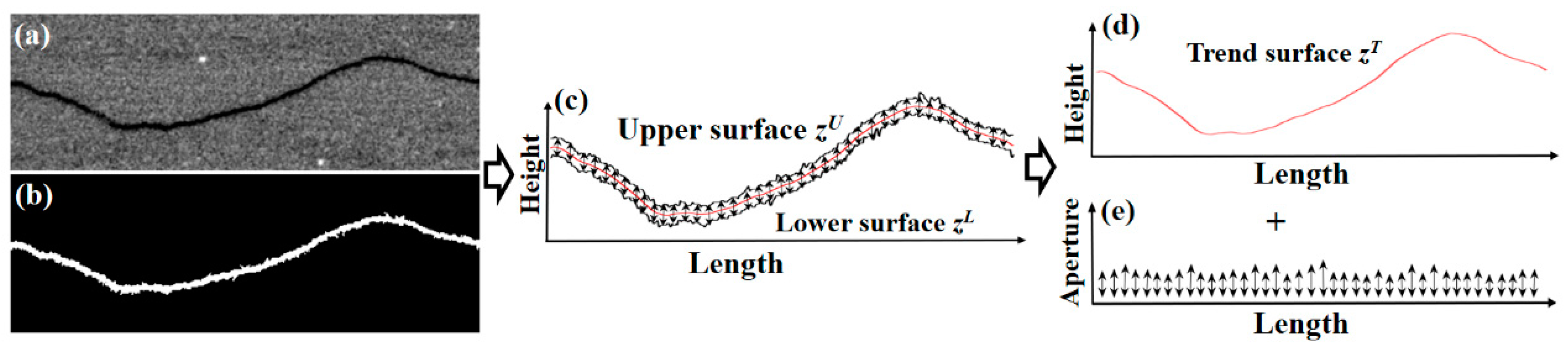
Figure 3.
A fracture model of 300 × 300 × 100 voxels with a trend surface surrounded by two fracture wall surfaces, where the three surfaces are generated in the same means with five pre-defined parameters: μb = 10 voxels, σb2 = 10, λb = 20 voxels, σT2 = 90, and λT = 120 voxels.
Figure 3.
A fracture model of 300 × 300 × 100 voxels with a trend surface surrounded by two fracture wall surfaces, where the three surfaces are generated in the same means with five pre-defined parameters: μb = 10 voxels, σb2 = 10, λb = 20 voxels, σT2 = 90, and λT = 120 voxels.
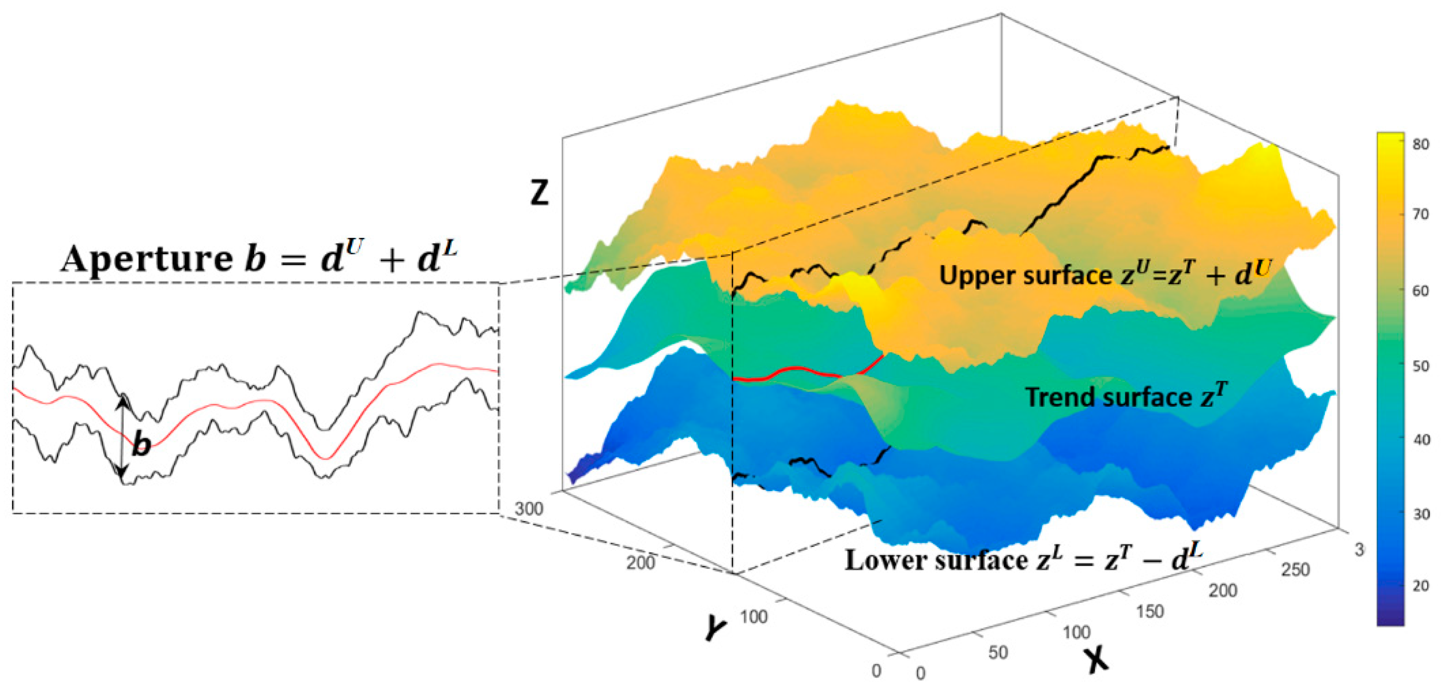
Figure 4.
Three fracture models of (a–c) generated by the mean-filter method with the same input morphological parameters as described in Figure 3, where the (red) trend surface is highlight by making transparent of a region of fracture void space.
Figure 4.
Three fracture models of (a–c) generated by the mean-filter method with the same input morphological parameters as described in Figure 3, where the (red) trend surface is highlight by making transparent of a region of fracture void space.

Figure 5.
LBM computing domain.

Figure 6.
Robustness of fracture modelling in terms of the relative errors on permeability.

Figure 7.
With fixed σb2 = 0 and λ = ∞, (a–c) demonstrate the influence of the trend surface of various σT2 but the same λT; (d–f) show the influence of the trend surface of various λT but the same σT2. The modelling trend surfaces are in red.
Figure 7.
With fixed σb2 = 0 and λ = ∞, (a–c) demonstrate the influence of the trend surface of various σT2 but the same λT; (d–f) show the influence of the trend surface of various λT but the same σT2. The modelling trend surfaces are in red.

Figure 8.
Relationships between the modified factor (fT) and the correlation lengths (λT) of (a–c) and the undulation coefficients (σT2) of (d–f) for three groups of fracture models of respective mean apertures of 5, 9, and 13 (in voxels), in which model parameters σb2 = 0, λb = ∞ are fixed. Where L presents the size (in voxels) of fracture models in X or Y direction. The black dotted lines are the fitting curves for the data lines for models of σT2 = 170 or λT/L = 120/300. The symbol R2 denotes the extent of the curves fitting the data.

Figure 9.
A plot of 75 triples of fT, σT2 and λT/L for 75 fractures in the three groups and a fitted surface.
Figure 9.
A plot of 75 triples of fT, σT2 and λT/L for 75 fractures in the three groups and a fitted surface.
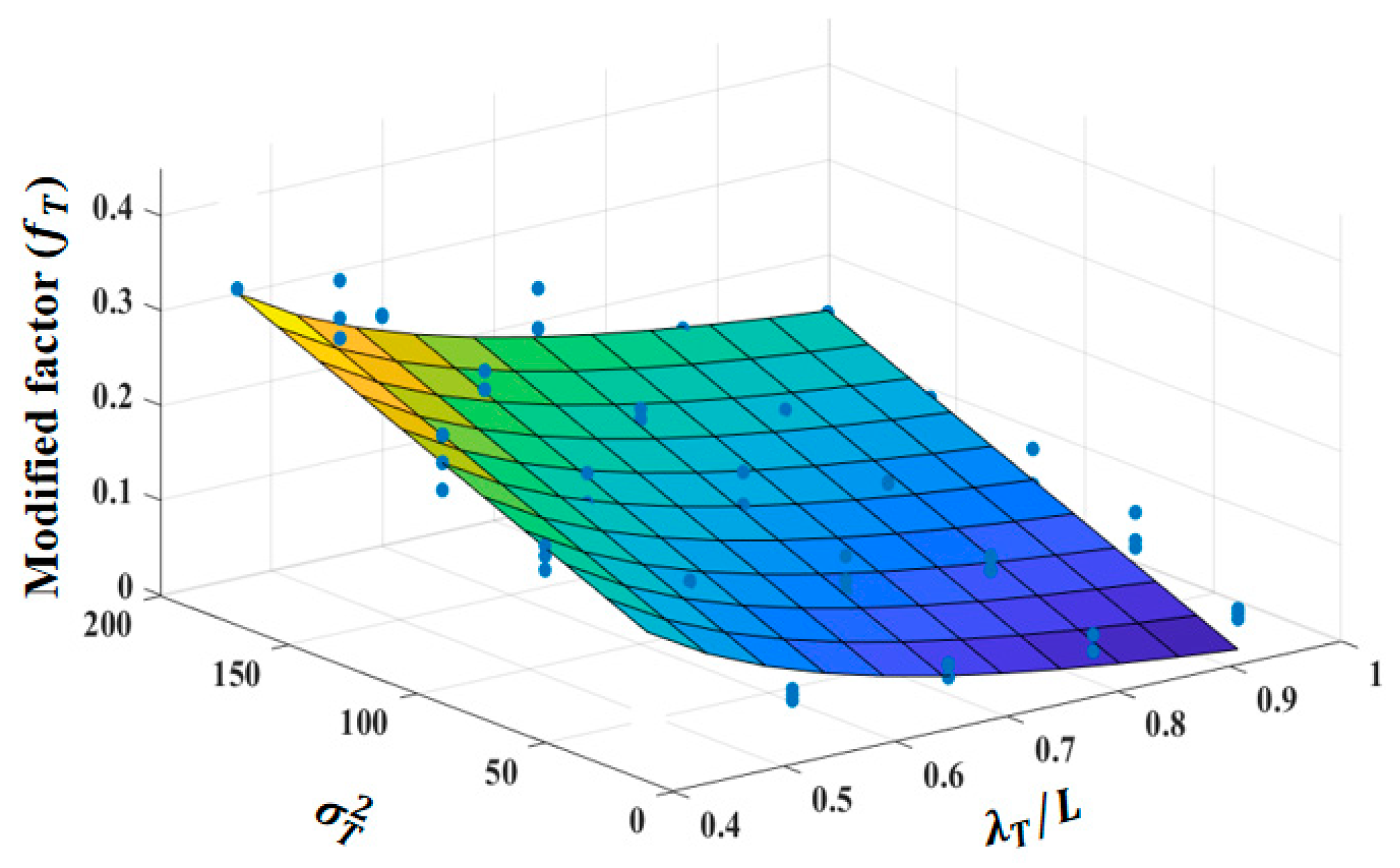
Figure 10.
With fixed σT2 = 0 and λT = ∞, (a–c) demonstrate the influence of fracture apertures with various σb/μb but the same λb; and (d–f) show the influence of fracture apertures with various λb but the same σb/μb. The modelling trend surfaces are in red.
Figure 10.
With fixed σT2 = 0 and λT = ∞, (a–c) demonstrate the influence of fracture apertures with various σb/μb but the same λb; and (d–f) show the influence of fracture apertures with various λb but the same σb/μb. The modelling trend surfaces are in red.

Figure 11.
Relationships between the modified factor (fb) and aperture correlation length (λb) of (a–c) and fracture wall roughness (σb/μb) of (d–f) for three groups of fracture models with the respective mean apertures of 5, 9, and 13 (in voxels), in which two trend surface parameters are set as to σT2 = 0, λT = ∞. Where L presents the fracture size in X or Y direction, and the black dotted lines are the fitted curves for three corresponding black solid lines for fracture models of σb/μb = 0.5 or λb/L = 6/300.
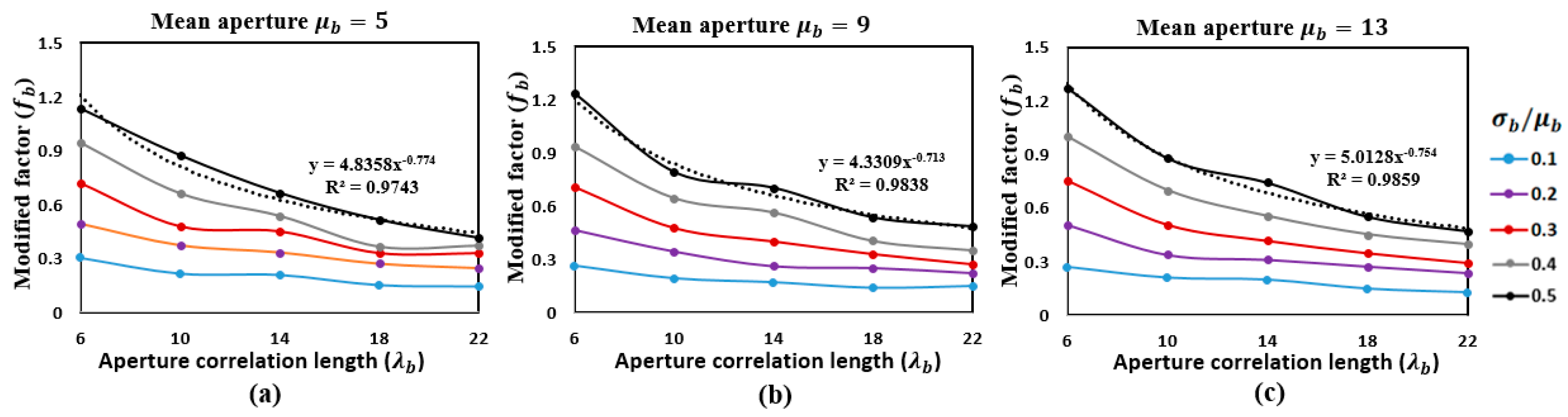
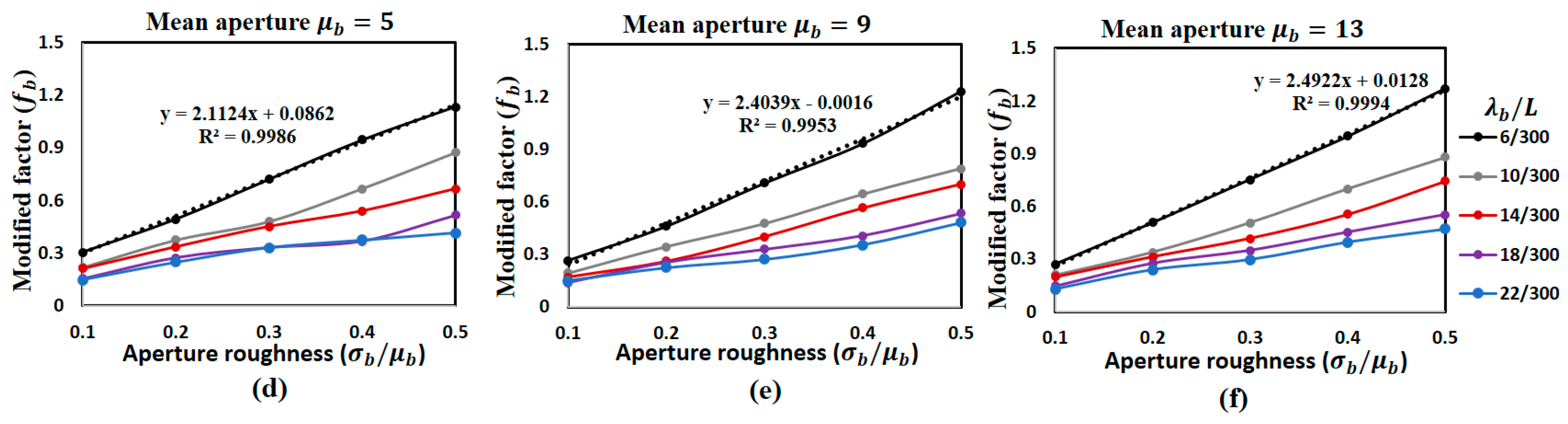
Figure 12.
Plot of 75 triples of fb, σb/μb and λb/L for 75 fracture models in the three groups and a fitted surface.
Figure 12.
Plot of 75 triples of fb, σb/μb and λb/L for 75 fracture models in the three groups and a fitted surface.
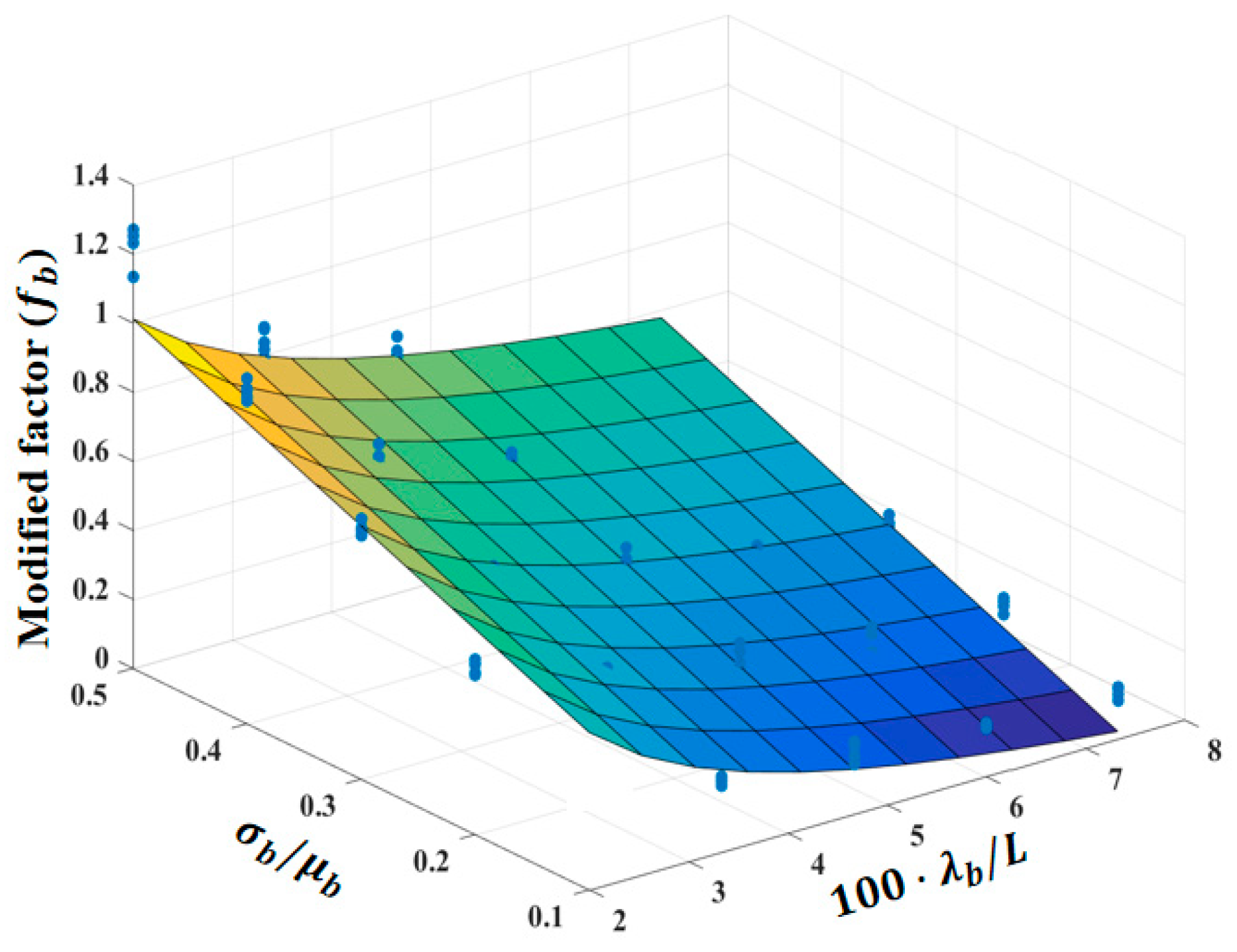
Figure 13.
Illustration of the accumulated influence: four fracture models of (a–d) for various σT2 and λT with the same (μb, σb/μb, λb) = (13, 0.5, 22); four fracture models of (e–h) for various σb/μb and λb with the same (μb, σT2, λT) = (13, 100, 120). The red curve represents the trend surfaces.
Figure 13.
Illustration of the accumulated influence: four fracture models of (a–d) for various σT2 and λT with the same (μb, σb/μb, λb) = (13, 0.5, 22); four fracture models of (e–h) for various σb/μb and λb with the same (μb, σT2, λT) = (13, 100, 120). The red curve represents the trend surfaces.
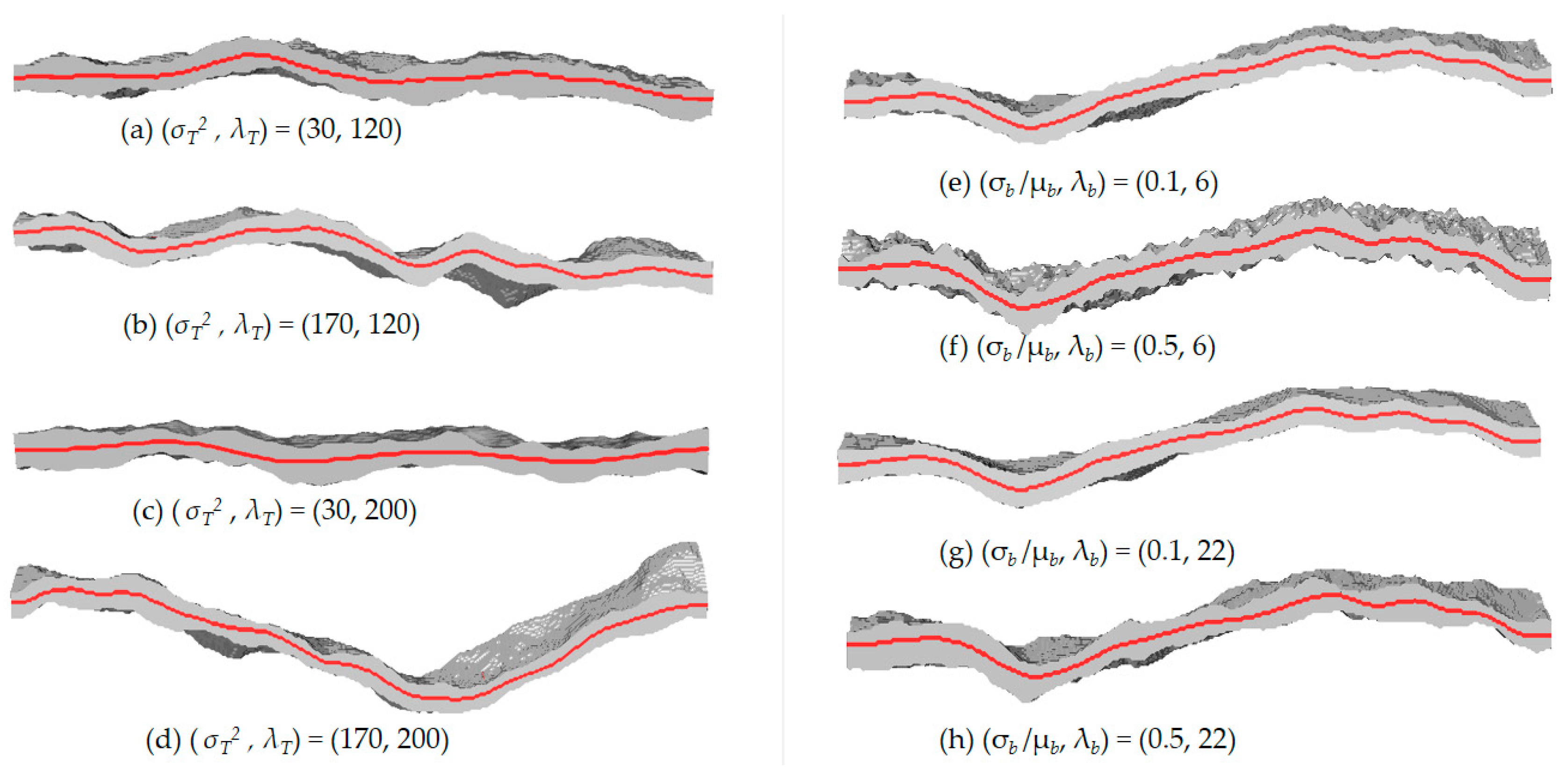
Figure 14.
The fitted surface for the data of triple (fT, fb, f) with the equation of Equation (13).
Figure 14.
The fitted surface for the data of triple (fT, fb, f) with the equation of Equation (13).

Figure 15.
Seven slice images of CT images of 10243 voxels scanned on 5 shale and 2 sandstone cores, a sub-image that contains a single fracture is cropped out from each CT image, having a smaller dimension of 300 × 300 × 100 voxels.
Figure 15.
Seven slice images of CT images of 10243 voxels scanned on 5 shale and 2 sandstone cores, a sub-image that contains a single fracture is cropped out from each CT image, having a smaller dimension of 300 × 300 × 100 voxels.

Table 1.
The characteristic parameters of eight different fracture samples presented in the green box of Figure 15 and the sample permeabilities calculated from LBM, cubic law and modified cubic law.
Table 1.
The characteristic parameters of eight different fracture samples presented in the green box of Figure 15 and the sample permeabilities calculated from LBM, cubic law and modified cubic law.
| Samples | μb (μm) | σb/μb | λb (μm) | σT2 | λT (μm) | KLB (mD) | Kcl (mD) | Kmcl (mD) | εcl (%) | εmcl (%) |
|---|---|---|---|---|---|---|---|---|---|---|
| SA1A | 5.03 | 0.26 | 6 | 160.75 | 150 | 1110.49 | 2108.41 | 982.76 | 89.86 | −11.5 |
| SA1B | 5.28 | 0.19 | 6 | 90.60 | 150 | 1443.05 | 2323.20 | 1232.62 | 60.99 | −14.58 |
| SA1C | 5.52 | 0.25 | 10 | 231.2 | 200 | 1157.60 | 2539.20 | 1297.74 | 119.35 | 12.11 |
| SA2 | 10.45 | 0.20 | 20 | 14.40 | 150 | 6166.89 | 9100.21 | 6372.08 | 47.57 | 3.33 |
| SA3 | 11.75 | 0.16 | 10 | 161.14 | 200 | 6705.99 | 11,505.21 | 7434.62 | 71.57 | 10.87 |
| SA4 | 6.74 | 0.18 | 10 | 45.99 | 150 | 2665.43 | 3785.63 | 2389.23 | 42.03 | −10.36 |
| SA5 | 11.45 | 0.14 | 10 | 18.6 | 150 | 8102.42 | 10,925.21 | 8551.35 | 34.84 | 5.54 |
| SB1 | 5.25 | 0.18 | 7 | 94.25 | 150 | 1468.85 | 2296.88 | 1271.76 | 56.37 | −13.4 |
| SB2 | 10.81 | 0.30 | 20 | 70.5 | 140 | 5689.30 | 9738.01 | 5599.80 | 71.16 | −1.57 |
© 2019 by the authors. Licensee MDPI, Basel, Switzerland. This article is an open access article distributed under the terms and conditions of the Creative Commons Attribution (CC BY) license (http://creativecommons.org/licenses/by/4.0/).
Share and Cite
MDPI and ACS Style
Li, X.; Jiang, Z.; Min, C. Quantitative Study of the Geometrical and Hydraulic Characteristics of a Single Rock Fracture. Energies 2019, 12, 2796. https://doi.org/10.3390/en12142796
AMA Style
Li X, Jiang Z, Min C. Quantitative Study of the Geometrical and Hydraulic Characteristics of a Single Rock Fracture. Energies. 2019; 12(14):2796. https://doi.org/10.3390/en12142796
Chicago/Turabian StyleLi, Xinling, Zeyun Jiang, and Chao Min. 2019. "Quantitative Study of the Geometrical and Hydraulic Characteristics of a Single Rock Fracture" Energies 12, no. 14: 2796. https://doi.org/10.3390/en12142796
Note that from the first issue of 2016, this journal uses article numbers instead of page numbers. See further details here.