Control of a Multiphase Buck Converter, Based on Sliding Mode and Disturbance Estimation, Capable of Linear Large Signal Operation

Abstract

Power-hardware-in-the-loop systems enable testing of power converters for electric vehicles (EV) without the use of real physical components. Battery emulation is one example of such a system, demanding the use of bidirectional power flow, a wide output voltage range and high current swings. A multiphase synchronous DC-DC converter is appropriate to handle all of these requirements. The control of the multiphase converter needs to make sure that the current is shared equally between phases. It is preferred that the closed-loop dynamic model is linear in a wide range of output currents and voltages, where parameter variations, control signal limits, dead time effects, and so on, are compensated for. In the case presented in this paper, a cascade control structure was used with inner sliding mode control for phase currents. For the outer voltage loop, a proportional controller with output current feedforward compensation was used. Disturbance observers were used in current loops and in the voltage loop to compensate mismatches between the model and the real circuit. The tuning rules are proposed for all loops and observers, to simplify the design and assure operation without saturation of control signals, that is, duty cycle and inductor current reference. By using the proposed control algorithms and tuning rules, a linear reduced order system model was devised, which is valid for the entire operational range of the converter. The operation was verified on a prototype 4-phase synchronous DC-DC converter.

1. Introduction

The global transport sector is currently moving from fossil fuel vehicles to electrically driven vehicles (EV). An electric motor requires a power controller to control speed, torque and power. In addition to powering the motor, the controller can support the regeneration of the energy in the battery and, thus, establishes a two-way flow of energy. In order to increase efficiency and reduce size, controllers will be under constant development in the future. When testing a controller for EV and hybrid electric vehicles (HEV), real operating conditions are needed, which involves a battery. This battery should be preconditioned, which takes time. The high capacity batteries of today are lithium-based and very vulnerable to abuse. In case of failure, for example, high temperature, overcurrent, or mechanical intervention, they can catch fire, or, in the worst cases, even explode. The life expectancy of a battery depends on a number of cycles; as it ages, the characteristics change and the repeatability of tests is worse. Batteries are in the form of big packs, so the testing facility also needs enough room. A battery emulator (BE) is a solution to the problems mentioned. A real battery is replaced by a DC power supply, which has programmable characteristics. That way, different types of batteries can be emulated, simply by changing the battery model structure and parameters. Preconditioning is not needed, as in the case of real batteries, because the state of charge (SOC) is set in a program, and the emulator sets the corresponding output voltage. Repeatability of tests is better, because a BE always has the same characteristics for the same parameters.

The DC power supply for battery emulation should supply a high enough current to the motor controller, with a wide output voltage range that mimics a real battery. Power converters of the switching type are preferred as the power demand of the motor controller is high. Switching the power supply brings more noise into the circuit and the wanted characteristic of the dynamic is hard to achieve, especially in the case of big power swings, as is the case of an EV. The power flow is preferred to be bidirectional, as in HEV, where, for example, the battery is a power source as well as a power drain. The control algorithm of such a converter would operate it to behave according to a real battery model [1]. Because of the controller’s finite bandwidth, external disturbances, sensor noise, and an unmatched converter model, this can be achieved in a limited sense. The power supply for a BE should operate at a wide range of voltages (from empty to full battery) and with large current swings (transitions from no load to full load). Power converters, which are typically designed for the nominal operating point, behave differently at other operating points. When exposed to large signal change, they incorporate some nonlinear characteristics, like soft start and current limiting, which limit their performance, and, of course, the dynamic characteristics are different to those in small signal operation. These effects were described and analyzed for the case of a buck converter in a previous study [2]. Power converters can also exhibit unstable behavior in such cases. Nonlinearities in the forms of converter nonlinear characteristic, parameter nonlinear dependence (for example, inductance is dependent on current), control signal saturation, and dead time, effects in the transistor legs [3], impact the dynamical response and stability, so they can be significantly different than in the designed nominal case.. A controller for BE should compensate for these nonlinearities, so that the dynamical characteristic is operating point independent; if it is linear, the control design for battery model tracking can be simpler. The motor controller acts as a Constant Power Load (CPL), which is described as negative incremental resistance in the literature [4]. The behavior of a converter with such a load could become unstable, which the controller has to account for [5].

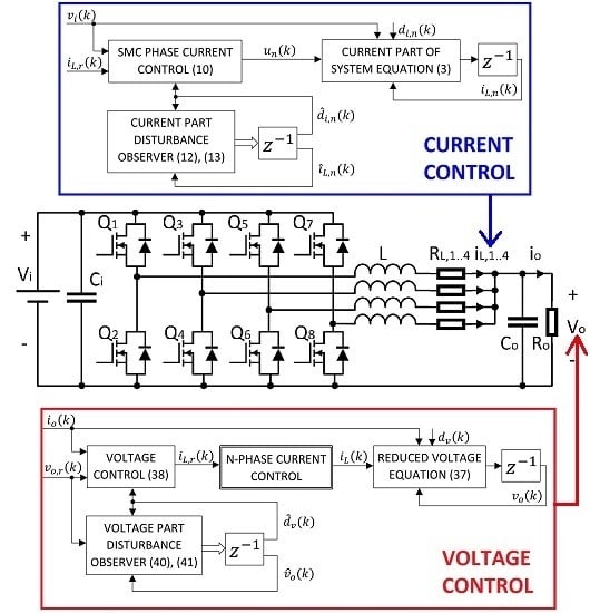
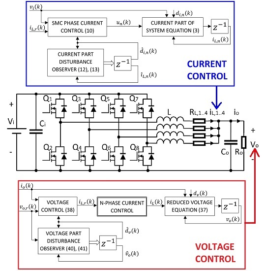
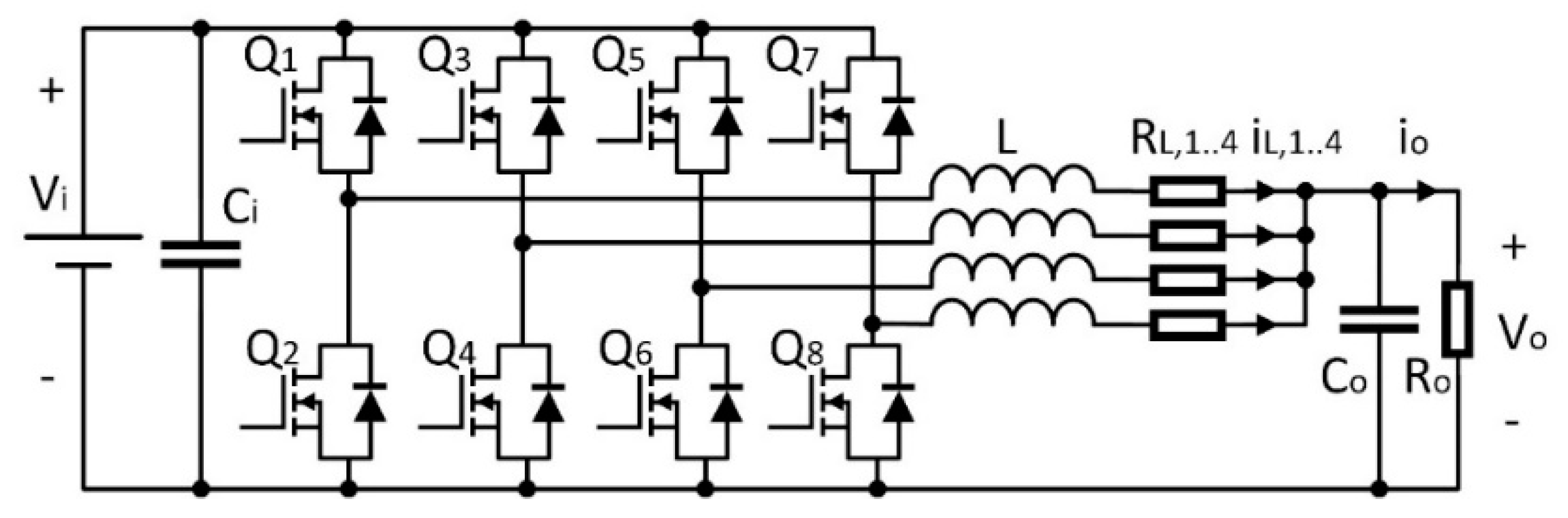
The aim of this work was to design a power converter control algorithm suitable for use in BEs. The power converter used was a multiphase buck converter (Figure 1), which is used widely for high power applications in different configurations, especially in the EV and HEV sector [6,7,8,9,10]. Because all the active elements are MOSFETs (Metal Oxide Semiconductor Field Effect Transistor—$Q_{\mathrm{1\dots 8}}$), topology is synchronous and power flow is bidirectional. Other benefits of such a converter are current sharing between phases, and low current ripple on output, and it can be used in buck and boost configurations. As the phases of such a converter are never completely identical, currents will not be completely balanced without a special balancing algorithm, which is one of the main problems of such a topology. For any balancing algorithm, phase currents need to be measured directly, or estimated from voltage drop on the equivalent series resistance (ESR) of the input [11] or output [12] capacitors. Direct measurement is preferred, as the latter puts a limit on the duty cycle. It is also important to sample the currents at the right moments, which was investigated in a previous study [13]. There is a lot of ongoing research on balancing algorithms, and solutions can be divided into two major types:

• Current balancing by varying duty ratios on phases.
• A current control loop on each phase with the same reference current for all phases.

For the first type, balancing is implemented by comparing a corresponding phase current to the average of currents, or to the master phase current, which is fixed or selected dynamically [14]. The method may work well, but the dynamic operation is not very predictable, which can be a problem if one wants to get a system dynamic description. Peak current mode control fits into the second type of balancing algorithms; it is attractive and used widely because of the high bandwidth [15]. Another benefit is that the effect of input voltage on the output is cancelled in one cycle and the system order is reduced. However, the model presented in a previous study [16] is dependent on the rising slope of the inductor current, which means it is dependent on the operating point—input and output voltage. This nonlinearity is not desirable for emulation purposes, where the converter’s output voltage range is wide. There are some other variants, like current mode control based on integral values [10,17] and average current mode control [18], but their model descriptions are also nonlinear. To give an operating point independent dynamic operation, feedforward blocks can be combined with classical Proportional-Integral (PI) controllers, as in Karimi et al. [7]. However, the integral part in the controller adds undesirable effects [19] to the system; the most problematic is control signal saturation, leading again to a nonlinear model. This implies large overshoots, slow settling time and control signal saturation, which is undesirable for emulation purposes, as the dynamic model becomes nonlinear, and it is not possible to find its inverse. One method to reduce the impact has been proposed in the form of constrained Proportional-Integral-Derivative (PID) algorithms [20].

Nonlinear control methods need to be used to gain a globally linear control model. Sliding mode control (SMC) is one such method [21], and it is being used in switching converters because of its robustness, stability, transient performance and simple implementation. In SMC, states of a system will reach the sliding surface, $\sigma =0$, from any initial condition in finite time and stay on it. System stability is, therefore, proven globally, and system dynamics can be prescribed for large signal changes. SMC has already been applied to multiphase converters, mainly with one master sliding surface for voltage control and slave sliding surfaces for phase current control. In an earlier work [22] these sliding surfaces make sure control signals of phases follow each other. The drawback, however, is lack of current control, so current sharing needs to be implemented separately. A similar procedure was used in another work [23], where switching frequency also needed to be controlled. Constant switching frequency SMC [5] is preferable, because of easier filter design and component efficiency optimization. Another way of controlling currents is by incorporating them into sliding surfaces. In previous studies [24,25] current sharing has been achieved by incorporating the average of currents into the sliding surfaces of each phase. Because surfaces are coupled, the dynamics of such a system are hard to describe in a reduced order model, which is preferable for emulation purposes. An interesting point of the principle is the voltage control part that is included in all surfaces, so the configuration can be thought of as multi-master. A similar structure was used in an earlier study [26]. When a phase malfunctions, voltage remains under control of the sliding surfaces of other phases. However, there are 3 parameters which can be difficult to tune. A better approach to controlling the power factor in a multiphase configuration was used in another study [27], where one reference current was applied to the sliding surfaces of all phases. This way, phases were decoupled from each other, and current control could be designed separately. This resulted in a simpler model, and is appropriate for emulation algorithms. An interesting use of sliding mode to control the current part of a single-phase buck converter is described in another work [28], where the inner current loop is controlled by the sliding surface, and the outer loop is an ordinary proportional-integral (PI) controller. It could be applied to multiphase converters, where they would share the same reference current. The drawback of the proposed algorithm is that it is based on one-step reaching of the sliding surface, which, in turn, means higher control effort and saturated control signals in the reaching phase, resulting in a nonlinear model. To cope with this problem, different variants of SMC have been proposed, based on a reaching law, such as Gao’s approach [29] and the linear reaching law [30]. By prescribing system dynamics in the reaching phase, control parameters can be designed in a way that the control signal is never saturated (the duty cycle is always within $\left[0,1\right]$) and the closed-loop dynamics are globally linear, also for large signal operations. This is different from conventional designs, where control is designed in the sliding surface, but, while reaching it, the control signal can be in saturation, and the system dynamics are different. Another solution to the problem can be found in another class of control algorithms, model predictive control (MPC) [8,31], which are also used for battery emulation purposes. The algorithm searches for control solutions inside bounds to prevent saturation. The disadvantage of this approach is computational complexity, making it inappropriate for use in digital signal processor (DSP)-controlled power converters. Moreover, in some cases, this method fails to find a solution [8], and the control signal is still saturated.

Nearly all of the mentioned sliding mode control algorithms for multiphase converters are based on an ideal model, where model uncertainties and unmatched phases are not accounted for. Unmatched characteristics can be compensated for by incorporating the integrative state in the sliding surface, similarly to the aforementioned linear PI controllers. This was applied to power converters in previous works [32,33], for discrete SMC, and this is called integral sliding mode (ISM) [34], where the integral part will make sure that the system reaches the sliding surface despite the uncertainties. However, as already mentioned for linear systems control theory, the integral part has its drawbacks [19], which are also manifested in ISM as integral dynamics in the form of large overshoots; slow settling time is also added to the system when the model matches the real system perfectly. Disturbance compensation, on the other hand, makes no intervention in the system when the model is matched. The observed disturbance value is bounded, unlike the integral, which can reach infinite values and requires anti-windup schemes. In Zongxiang et al. [35], the disturbance observer was used, along with the ISM, for motor control. However, the integral part was not eliminated completely, only its impact on the system dynamics was reduced. In Marcos-Pastor et al. [36], the integral part was completely replaced by the disturbance estimate for the magnetic levitation system, and its superior performance was shown. Some improvements of the method were presented in another study [37], where disturbance dynamics were also accounted for in the control algorithm. While SMC with a disturbance observer is used in various fields, there are only a few reported examples of its usage for controlling DC/DC converters. In a previous study [38], load current was an estimated disturbance, and the converter was controlled in a cascade of super-twisting-algorithms (STAs), which are based on SMC. In another study [39], the load resistance variation disturbance was estimated and used in terminal-sliding-mode (TSM) control of a buck converter. In another earlier study [40], disturbances of input voltage and load resistance are estimated by a linear observer, and used in SMC for a half bridge isolated converter. In another study [41], a disturbance estimate was used in the sliding surface to control a buck converter. However, for mismatched disturbances, integral state was still used, leading to the abovementioned problems.

The main contribution of this paper is a control for a multiphase buck converter that fits into the class of SMC algorithms. The aim was to control the converter appropriately for later use in battery emulation algorithms for EV. The control is based on cascade control with N identical inner sliding surfaces for inductor currents and an outer voltage control loop with output current feedforward. With the same current reference on all sliding surfaces, equal current sharing was accomplished. To steer states towards the sliding surface, the linear reaching law was used [30], which is based on Gao’s approach [29], but without the chattering effect. It will be shown, by using this approach, that control parameters can be designed in such a way that the control signal is never saturated (the duty cycle is always within $\left[0,1\right]$). By accounting for control limits in the design phase, the SMC design of this work resulted in a computationally simple control law, which can easily be applied to DSP processors, compared to MPC [8,31], which requires more computationally powerful processors. To compensate for model uncertainties and mismatch between phases, a disturbance observer of the Luenberger type, similar to the one in previous studies [36,41,42], was used, which made it possible to achieve zero steady state current error. The observer was of the linear type, which is simpler, and does not generate an undesired chattering effect like the sliding type observer used in a previous study [39]. Observer stability was proven with the linear system theory, and was easily implementable on digital controllers. Estimated disturbance was bounded, so the calculated control signal never went into saturation, as can be the case when using integral states [19,34]. The outer voltage loop was of proportional type, with feedforward of the output current that was measured. To compensate for the model’s mismatch in the voltage part, an observer was used of the same structure as in the case of the current part. In contrast to previous studies [38], the observer acted on a closed loop equation rather than on a system model. In contrast to another study [40], where the observer and controller were based on continuous domain, in this work they are discrete and directly applicable to DSP implementation. In discrete form, implementation is even simpler, because of the elimination of derivative calculations. A similar disturbance observer was used in another study [41], where a disturbance estimate was used in the sliding surface to control a buck converter, but for mismatched disturbances, the integral state was used, with all its drawbacks. In the present work, it will be shown that the integral state is not necessary; mismatched disturbances can also be cancelled effectively with a disturbance observer and appropriate tuning of current and voltage loop bandwidths. The rules are given to tune all parameters of the control system. The designed algorithms were tested on a prototype converter.

2. Multiphase Converter Modeling

A multiphase converter from Figure 1 can be modeled by the system Equation (1) with $N$ identical phase models, where $n\in \left\{1,2,\dots ,N\right\}.$ Phase inductor currents $i_{L,n}$ and output voltage $v_O$ are used as state variables. The inputs of the model $u_n$ represent the duty cycles of the pulse width modulators (PWM). Other variables are input voltage $v_i$ and output current $i_O$. The parameters for the current part are inductance $L$ and inductor ohmic resistance $R_L$, which can also include MOSFETs’ on-state resistances $R_{ds-ON}$ and current shunt resistances. $C_o$ in the voltage part of the model represents the output capacitance.

$$\begin{array}{c}\frac{d{i}_{L,n}}{dt}=-\frac{R_L}{L}{i}_{L,n}-\frac{1}{L}{v}_o+\frac{1}{L}{v}_i{u}_n\\ \frac{d{v}_o}{dt}=\frac{1}{C_o}{\displaystyle {\displaystyle \sum }_{n=1}^N}{i}_{L,n}-\frac{1}{C_o}{i}_o\end{array}$$

(1)

To design an SMC law, it needs to be transferred to the discrete domain. This can be evaluated by first order approximation of the z-transform [43], which gives a simple model (2), with sample time $T$, where $k$ represents the time step in sample intervals.

$$\begin{array}{c}{i}_{L,n}\left(k+1\right)=\left(1-\frac{R_{L}T}{L}\right)i_{L,n}\left(k\right)-\frac{T}{L}{v}_o\left(k\right)+\frac{T}{L}{v}_i\left(k\right)u_n\left(k\right)\\ v_o\left(k+1\right)=\frac{T}{C_o}{\displaystyle {\displaystyle \sum }_{n=1}^N}{i}_{L,n}\left(k\right)+v_o\left(k\right)-\frac{T}{C_o}{i}_o\left(k\right)\end{array}$$

(2)

In a real system there are some parameter uncertainties in the forms of inductor ohmic resistance deviation $\Delta R_L$ inductance drops and tolerances $\Delta L$, and capacitance deviation $\Delta C_o$. A real effective duty ratio is different from the ideal because of the dead times [3] and rise times of MOSFETs. There are some unknown disturbances in the form of sensor offsets and noise. This can all be lumped into disturbances for current part $d_{i,n}$ and voltage part $d_v$ and added to the model (2), obtaining a model with disturbances (3).

$$\begin{array}{c}{i}_{L,n}\left(k+1\right)=\left(1-\frac{R_{L}T}{L}\right)i_{L,n}\left(k\right)-\frac{T}{L}{v}_o\left(k\right)+\frac{T}{L}{v}_i\left(k\right)u_n\left(k\right)+d_{i,n}\left(k\right)\\ v_o\left(k+1\right)=\frac{T}{C_o}{\displaystyle {\displaystyle \sum }_{n=1}^N}{i}_{L,n}\left(k\right)+v_o\left(k\right)-\frac{T}{C_o}{i}_o\left(k\right)+d_{i,n}\left(k\right)\end{array}$$

(3)

3. Phase Current Control

Model (3) is of the $N+1$ order, where each phase current $i_{L,n}\left(k\right)$ is different, which can be a complex control problem from the parameter selection point of view, as well as closed loop dynamics could also be complex. With appropriate control algorithms for phase currents, they can be made equal, and the voltage model can be simplified to (4). This can be true if phase current control is faster than voltage control.

$$v_o\left(k+1\right)=\frac{NT}{C_o}{i}_L\left(k\right)+v_o\left(k\right)-\frac{T}{C_o}{i}_o\left(k\right)+d_v\left(k\right)$$

(4)

In Equation (3) it can be observed that the current model has nonlinearity on input, because of the multiplication of input voltage $v_i\left(k\right)$ with the duty ratio $u_n\left(k\right)$. The duty ratio $u_n\left(k\right)$ in a real system is limited, depending on the hardware; current sensors, MOSFET drivers, and so on. The converter presented here, neglecting dead times, enables operation from 0–1 duty cycle, so the assumed range of $u_n\left(k\right)$ will be on the interval $\left[0,1\right]$. Control signals outside of this range would result in duty cycle limiting and saturation, which implies a nonlinear model. It would be hard to find an inverse of such a model, which is desired for emulation algorithms. Another problem is disturbances $d_{i,n}\left(k\right)$, which are different and unknown. Despite disturbances, phase currents should have equal values in the stationary state, which implies accurate model description (4), distributed heating in the circuit, and efficient use of components.

3.1. Sliding Mode Current Control

Sliding mode control is a nonlinear control method, which is robust to model uncertainties [44] and performs well with large signal changes. The basis of this method is a prescribed sliding surface $\sigma$, made from controlled variables. The system variables are steered to reach the sliding surface and stay on it. The conventional method of implementing the SMC control is by using a relay of the signum function given along the sliding surface. For switching power converters, this results in unpredictable frequency, so the PWM-based continuous SMC [45] is more appropriate. The converter can be operated with fixed switching frequency and control signal governing system to follow ideal sliding dynamics—quasi SMC.

The control used in this paper is based on $N$ identical sliding surfaces (5), where $n$ is the phase index. All surfaces use the same reference current $i_{L,r}$, and compare it to the phase current $i_{L,n}$. Sliding surface ${\sigma }_n$ is like in [28], where the reference current is compared to the phase current.

$${\sigma }_n\left(k\right)=i_{L,r}\left(k\right)-i_{L,n}\left(k\right)$$

(5)

An equivalent control in a previous study [28] was evaluated by setting $\sigma \left(k+1\right)=0$, the so-called “one-step reaching”, but this is undesirable, as it results in large control signals, leading to limiting, and making the dynamics become nonlinear and noninvertible. Different reaching laws [30,46,47] can be applied to prevent overlarge control effort and to control the reaching phase of SMC. Among them, the linear reaching law (6) is simple and linear, meaning the closed loop system description will be linear in a global sense. The linear reaching law (6) is based on Gao’s reaching law [29] without the switching part to eliminate chattering. Sample time independent convergence rate parameter $q$ determines convergence speed in the reaching phase. For the simplification of equations, it will be replaced by sample time-dependent equivalent $Q$ in the following derivations.

$${\sigma }_n\left(k+1\right)=\left(1-qT\right){\sigma }_n\left(k\right),\mathrm{where}qT=Q\in \left(0,1\right)$$

(6)

There are, however, some improvements in the approach, in the form of variable convergence parameters in [48,49], but they result in nonlinearities in the closed loop description, so they are not applicable here. By combining the sliding surface (5) with the reaching law (6), Equation (7) can be obtained.

$$i_{L,r}\left(k+1\right)-i_{L,n}\left(k+1\right)=\left(1-Q\right)(i_{L,r}\left(k\right)-i_{L,n}\left(k\right))$$

(7)

Then, by introducing (3) into (7) and solving for $u_n$, the equivalent control law (8) can be derived.

$$u_n\left(k\right)=\frac{L}{T{v}_i\left(k\right)}\left(i_{L,r}\left(k+1\right)+\left(Q-1\right)i_{L,r}\left(k\right)+\left(-Q+\frac{R_{L}T}{L}\right)i_{L,n}\left(k\right)+\frac{T}{L}{v}_o\left(k\right)-d_{i,n}\left(k\right)\right)$$

(8)

The control law derived (8) is not implementable, because disturbance $d_{i,n}\left(k\right)$ is not known. By removing it from the control law, that is, $d_{i,n}\left(k\right)=0$, reaching dynamics (9) can be obtained. It deviates from (7) by $d_{i,n}\left(k\right)$, so additional measures need to be implemented for cancelling its impact.

$$i_{L,r}\left(k+1\right)-i_{L,n}\left(k+1\right)=\left(1-Q\right)(i_{L,r}\left(k\right)-i_{L,n}\left(k\right))-d_{i,n}\left(k\right)$$

(9)

3.2. Design of a Disturbance Observer for Current Control

According to (9), unknown disturbance alters the reaching law, and moreover, as $k\to \infty$, the system does not reach the sliding surface, it only converges to the disturbance’s steady state value $d_{i,n}(\infty )$. The first solution to the problem can be modification of the sliding surface, with the addition of an integral term, called the integral sliding mode (ISM) [34]. However, the integral has some drawbacks, observed from the linear systems control theory [19], which also manifest themselves in ISM [37]. Integral dynamics are also added to the system when the model matches the real system perfectly. This implies large overshoots, slow settling time, and so on. As the maximum value of the integral is hard to predict, it can result in control signal saturation. The second solution to deal with disturbance is to prescribe model uncertainties, and include their assumptions in the sliding surface, as in [48,50]. The control signal can, therefore, be predicted in the development phase of control to be always within the interval $\left[0,1\right]$, so there is no need for limitation. However, without the use of switching functions in the sliding surface, it is hard to achieve zero steady state error, where system states are only in the vicinity of the sliding surface. Disturbance estimation and rejection techniques [19,36,51] solve the drawbacks of both solutions mentioned. As disturbance estimate has a finite and predictable value, the control signal can be designed to be always inside the bounds. The disturbance observer can estimate steady state disturbances, so the system can reach the sliding surface, not just the vicinity of it. Disturbance estimation is especially attractive in discrete time control [42], because of the easier implementation of delayed states, compared with computing state derivatives, as in the case of continuous time control [51]. With the use of estimated disturbance ${\widehat{d}}_{i,n}$ instead of real $d_{i,n}$, the control law (8) can be changed. It can also be assumed that the reference current is slow time varying, $i_{L,r}\left(k+1\right)\approx i_{L,r}\left(k\right)$, which all results in an implementable control law (10).

$$u_n\left(k\right)=\frac{L}{T{v}_i\left(k\right)}\left(Q{i}_{L,r}\left(k\right)+\left(-Q+\frac{R_{L}T}{L}\right)i_{L,n}\left(k\right)+\frac{T}{L}{v}_o\left(k\right)-{\widehat{d}}_{i,n}\left(k\right)\right)$$

(10)

By putting (10) into system Equation (3), the closed loop response of the system can be evaluated (11).

$$i_{L,n}\left(k+1\right)=\left(1-Q\right)i_{L,n}\left(k\right)+Q{i}_{L,r}\left(k\right)+d_{i,n}\left(k\right)-{\widehat{d}}_{i,n}\left(k\right)$$

(11)

It can be observed that the disturbance estimate cancels the disturbance; hence, the system reaches the sliding surface in steady state if the disturbance is matched. If all states of the system are measurable, disturbance can be estimated from the system model. It is convenient to estimate disturbance from closed loop dynamics (11), as a simple linear Luenberger observer type can be used with observer gain $l_i$ (12).

$${\widehat{d}}_{i,n}\left(k+1\right)={\widehat{d}}_{i,n}\left(k\right)+l_i\left(i_{L,n}\left(k\right)-{\widehat{i}}_{L,n}\left(k\right)\right)$$

(12)

Equation (13) is proposed to calculate the estimated current ${\widehat{i}}_{L,n}\left(k\right)$. It has a similar structure to (11), with the disturbance parts omitted. In the following analysis it will be proven that it can form a stable observer in conjunction with Equations (11) and (12).

$${\widehat{i}}_{L,n}\left(k+1\right)=\left(1-Q\right){\widehat{i}}_{L,n}\left(k\right)+Q{i}_{L,r}\left(k\right)$$

(13)

First, the current estimation error $e_i\left(k\right)$ and disturbance estimation error $e_d\left(k\right)$ variables are defined as (14).

$$\begin{array}{c}{e}_i\left(k\right)=i_{L,n}\left(k\right)-{\widehat{i}}_{L,n}\left(k\right)\\ e_d\left(k\right)=d_{i,n}\left(k\right)-{\widehat{d}}_{i,n}\left(k\right)\end{array}$$

(14)

By rewriting (14) for $k+1$, estimation errors are gained for the next time step (15).

$$\begin{array}{c}{e}_i\left(k+1\right)=i_{L,n}\left(k+1\right)-{\widehat{i}}_{L,n}\left(k+1\right)\\ e_d\left(k+1\right)=d_{i,n}\left(k+1\right)-{\widehat{d}}_{i,n}\left(k+1\right)\end{array}$$

(15)

Then, current estimation error for $k+1$ step (16) is derived by putting (11) and (13) into (15) and simplifying by (14).

$$e_i\left(k+1\right)=e_d\left(k\right)$$

(16)

The disturbance estimation error for $k+1$ step can follow the same derivation as used in [42], only the disturbance estimate (12) is different here. The real disturbance dynamics are unknown, but can be assumed by (17), where the incremental disturbance change is defined as $\Delta d_{i,n}\left(k+1\right)=d_{i,n}\left(k+1\right)-d_{i,n}\left(k\right)$.

$$d_{i,n}\left(k+1\right)=d_{i,n}\left(k\right)+\Delta d_{i,n}\left(k+1\right)$$

(17)

Putting (12) and (17) into (15) and simplifying by (14), the disturbance estimation error for $k+1$ step can be evaluated in (18).

$$e_d\left(k+1\right)=e_d\left(k\right)+\Delta d_{i,n}\left(k+1\right)-l_i{e}_i\left(k\right)$$

(18)

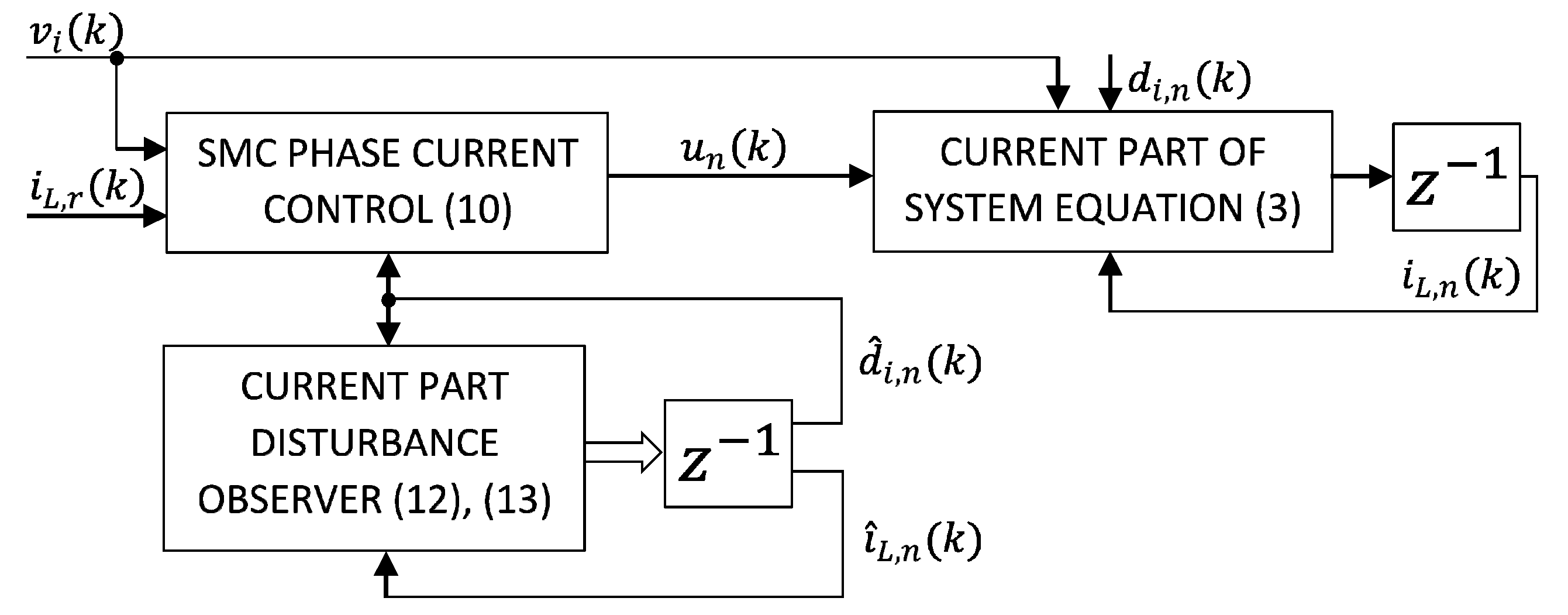
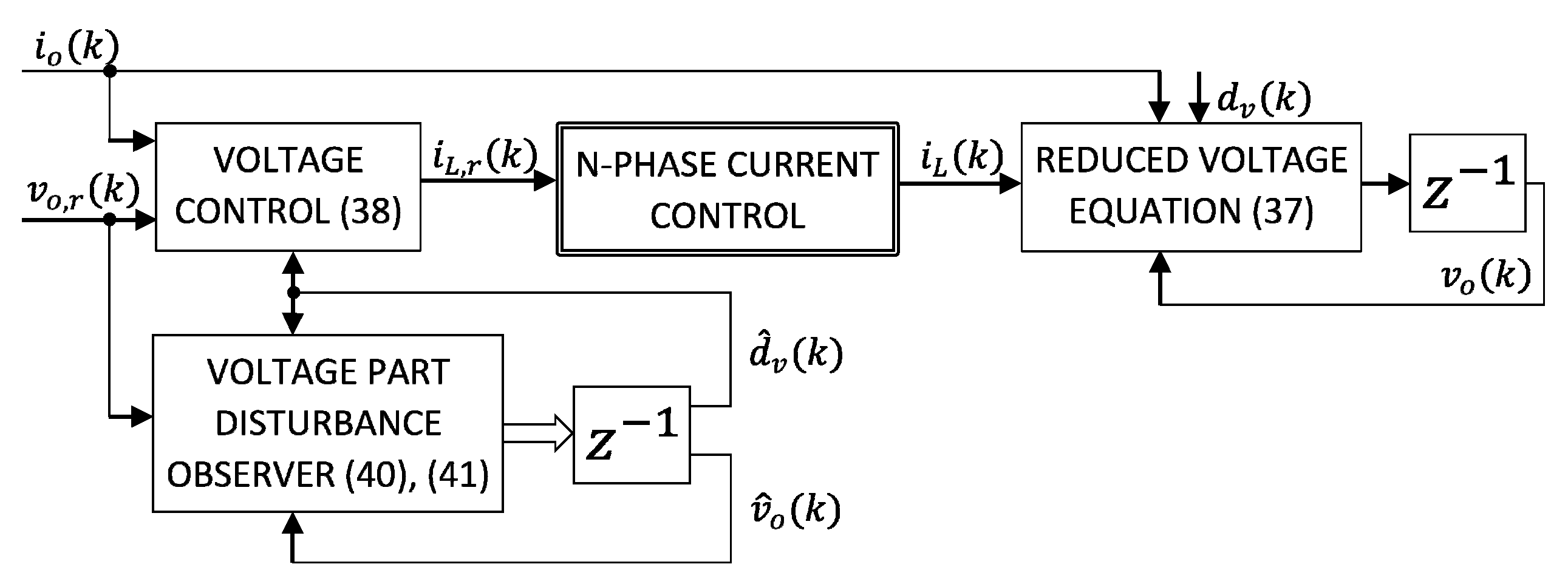
The final control diagram with SMC and the disturbance observer for phase current control is shown in Figure 2.

3.3. Proposed Rules to Tune the Sliding Mode Current Controller and the Disturbance Observer

For tuning controller parameter $Q$ and observer parameter $l_i$, first the tuning rules will be proposed, based on pole location analysis. Then, the second rule will be proposed, where operation inside control limits and operation without saturation effects is guaranteed. Equations (11), (16) and (18) can be compacted in the matrix form (19) with system matrix $A_i$ and system vectors $x_i$, $b_i$, $g_i$.

$$\underset{x_i\left(k+1\right)}{\underbrace{\left[\begin{array}{c}{i}_{L,n}\left(k+1\right)\\ e_d\left(k+1\right)\\ e_i\left(k+1\right)\end{array}\right]}}=\underset{A_i}{\underbrace{\left[\begin{array}{ccc}1-Q& 1& 0\\ 0& 1& -l_i\\ 0& 1& 0\end{array}\right]}}\underset{x_i\left(k\right)}{\underbrace{\left[\begin{array}{c}{i}_{L,n}\left(k\right)\\ e_d\left(k\right)\\ e_i\left(k\right)\end{array}\right]}}+\underset{b_i}{\underbrace{\left[\begin{array}{c}Q\\ 0\\ 0\end{array}\right]}}{i}_{L,r}\left(k\right)+\underset{g_i}{\underbrace{\left[\begin{array}{c}0\\ \Delta d_{i,n}\left(k+1\right)\\ 0\end{array}\right]}}$$

(19)

The system is linear, and stability can be checked by calculating eigenvalues ${\lambda }_i$ of the system matrix $A_i$ by (20), where I is the identity matrix.

$$\det \left({\lambda }_{i}I-A_i\right)=0$$

(20)

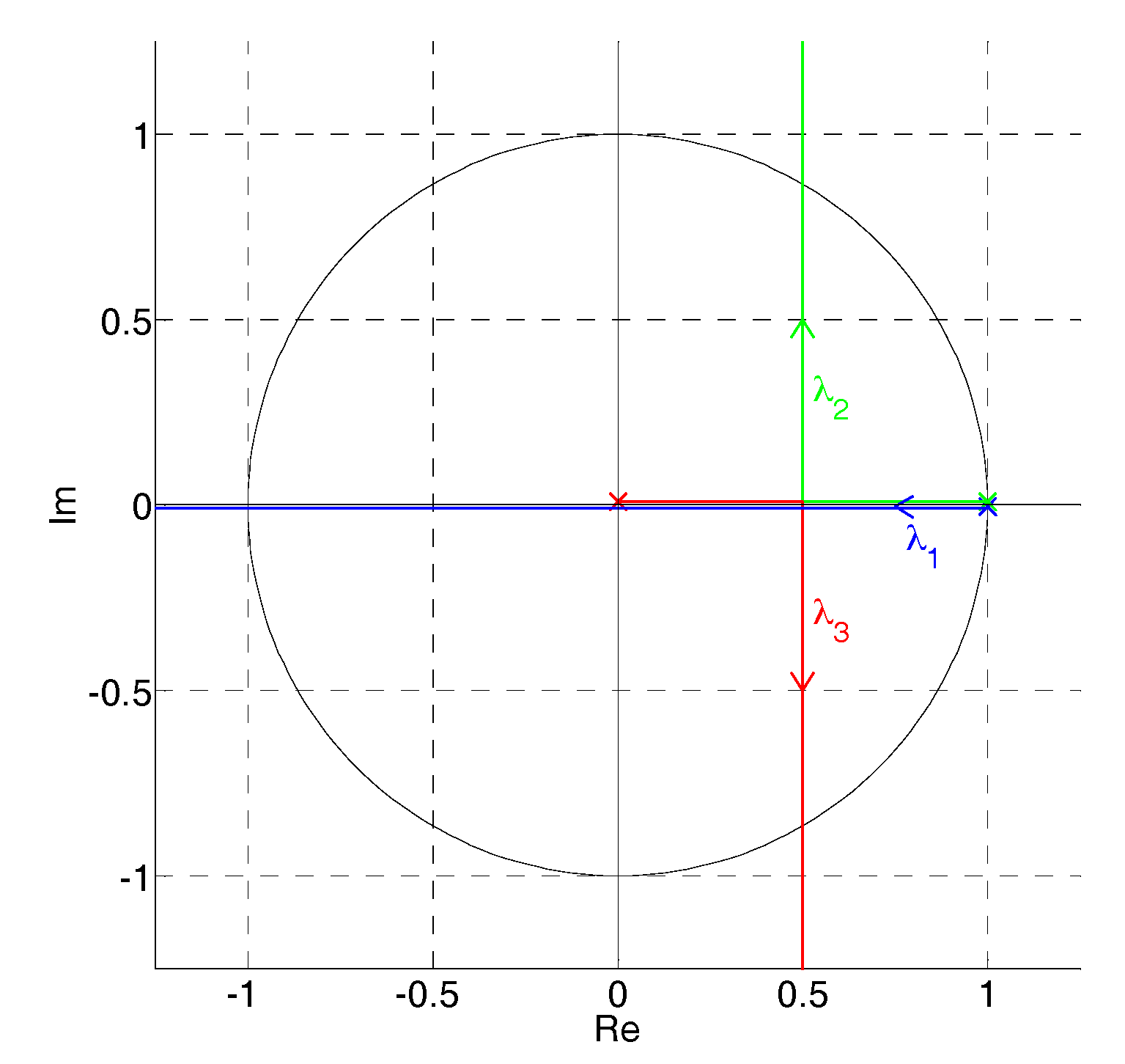
By putting (19) into (20), eigenvalues ${\lambda }_1$, ${\lambda }_{2,3}$, that represent system poles, are gained in (21). To be stable, all should be inside the unit circle. Without common parameters, sliding mode controller pole ${\lambda }_1$ and observer poles ${\lambda }_{2,3}$ do not depend on each other, so the poles can be treated separately from the stability point of view.

$$\begin{array}{c}{\lambda }_1=1-Q\\ {\lambda }_{2,3}=\frac{1}{2}\pm \frac{\sqrt{1-4L_i}}{2}\end{array}$$

(21)

Figure 3 shows how the poles move in the z-plane when $Q$ is increased from 0 to infinity, and $l_i$ is increased from 0 to infinity. Observer poles ${\lambda }_{2,3}$ do not affect controller stability, but in (19) it can be seen that the disturbance estimation error $e_d\left(k\right)$ affects controller response. The poles of controller and observer therefore need to be placed as far apart as possible, with the controller pole much closer to the unit circle. Thus, the dynamics of the controller are predominant. As poles ${\lambda }_{2,3}$ start from different locations, the optimal case would be to place them in ${\lambda }_{2,3}=\frac{1}{2}$. That way, the location of both poles would be far away from the unit circle, that is, they would be less dominant, with high natural frequency. Putting ${\lambda }_{2,3}=\frac{1}{2}$ into (21) gives the needed observer gain $l_i$ (22). That way, observer pole placement is solved analytically, and the observer parameter is independent of system parameters.

$$l_i=\frac{1}{4}$$

(22)

To tune the controller parameter $Q$, two major requirements should be fulfilled. From Figure 3, the first requirement is that the controller pole ${\lambda }_1$ is dominant, that is, separated enough from observer poles ${\lambda }_{2,3}$ and closer to the unit circle. The second requirement is for the control signal, that is, the duty ratio, to be always inside bounds, $u_n\left(k\right)\in \left[0,1\right]$. This way, it would be possible to gain reduced order dynamic description without saturation effects—nonlinearities. To make ${\lambda }_1$ dominant, it should be closer to the unit circle. To get some more understanding of poles, their natural frequencies ${\mathsf{\omega }}_1$,${\mathsf{\omega }}_{2,3}$ and damping ratio $\mathsf{\zeta }$ in continuous space ($\mathrm{s}$-domain) can be gained by equating eigenvalues with the equation for poles of the first order system (23) and second order system (24). By setting $\mathsf{\zeta }$ to 1, the observer’s poles are put to the same location on the real axis (${\lambda }_{2,3}=\frac{1}{2}$) and pole location Equation (24) is simplified to ${\lambda }_{2,3}=e^{-{\mathsf{\omega }}_{2,3}T}$, which is of the same structure as (23).

$$\mathrm{s}=-{\mathsf{\omega }}_1 \stackrel{z=e^{sT}}{\to }{\lambda }_1=e^{-{\mathsf{\omega }}_{1}T}$$

(23)

$$\mathrm{s}=-{\mathsf{\zeta }\mathsf{\omega }}_{2,3}\pm j{\mathsf{\omega }}_{2,3}\sqrt{1-{\mathsf{\zeta }}^2} \stackrel{z=e^{sT}}{\to }{\lambda }_{2,3}=e^{-{\mathsf{\zeta }\mathsf{\omega }}_{2,3}T\pm j{\mathsf{\omega }}_{2,3}T\sqrt{1-{\mathsf{\zeta }}^2}} \stackrel{\mathsf{\zeta }=1 }{\to }{\lambda }_{2,3}=e^{-{\mathsf{\omega }}_{2,3}T}$$

(24)

That way, pole dominance can be assured only by setting poles’ natural frequencies (${\mathsf{\omega }}_1$ and ${\mathsf{\omega }}_{2,3}$) appropriately. For ${\lambda }_1$ to be dominant, its natural frequency ${\mathsf{\omega }}_1$ should be lower than the pole’s ${\lambda }_{2,3}$ natural frequency ${\mathsf{\omega }}_{2,3}$. Generally, a ratio of 5 or more is sufficient, so (25) can be used as a basic rule for further tuning.

$${\mathsf{\omega }}_{2,3}\ge 5{\mathsf{\omega }}_1$$

(25)

By solving ${\mathsf{\omega }}_1$ from (23) and ${\mathsf{\omega }}_{2,3}$ from (24), using (21), (22) and putting all into (25), $Q$ can be derived (26).

$$Q\le 1-\sqrt[5]{{\lambda }_{2,3}}=0.13$$

(26)

As value $Q$ depends on ${\lambda }_{2,3}$, which has been determined before, parameter tuning selection has been greatly simplified. However, this is the first requirement for tuning the SCM, which assures its dominance over the observer.

The second requirement, $u_n\left(k\right)\in \left[0,1\right],$ is needed to guarantee that the control signal will never be saturated and that globally linear system dynamics can be gained. This is different than in the general procedure, where $u_n\left(k\right)$ can be calculated outside the range and then limited. The philosophy has been used in the design of multiphase converters for transient performance, where converters’ bandwidths are designed so that voltage spikes are symmetrical [52,53]. In the work presented here, the controller was designed with bandwidth based on a physical system, but it should be noted that in the sources mentioned a different approach is also possible; to design a physical system—inductances based on the required control bandwidth. The idea from previous works [52,53] is that the control signal can be guaranteed globally inside bounds ($u_n\left(k\right)\in \left[0,1\right])$ when the inductor current slope $\frac{d{i}_L}{dt}$, demanded in the control algorithm, is never higher than the physical system can handle, that is, it is dependent on inductance. For discrete time system description, this can be translated into incremental current change $\Delta i_{L,n}\left(k+1\right)$, expressed in (27).

$$\Delta i_{L,n}\left(k+1\right)=i_{L,n}\left(k+1\right)-i_{L,n}\left(k\right)$$

(27)

Putting closed loop current dynamics ($i_{L,n}\left(k+1\right)$) from (19) into (27) and assuming $e_d\left(k\right)\approx 0$ (this is valid, as the observer’s bandwidth is higher than the controller’s (25)), the worst case of value of $\Delta i_{L,n}\left(k+1\right)$, that is, $\Delta I_{L,C}$, is gained in (28). By selecting the appropriate border value of $i_{L,r}$, that is, $I_{L,r}$, and border value of $i_L$, that is, $I_L$, the equation can give the worst case demanded incremental current change $\Delta I_{L,C}$ from the controller.

$$\Delta I_{L,C}=Q{I}_{L,r}-Q{I}_L$$

(28)

Putting open loop current dynamics ($i_{L,n}\left(k+1\right)$), from (2) into (27), the worst case of value of $\Delta i_{L,n}\left(k+1\right)$, that is, $\Delta I_{L,P}$ is gained in (29). By selecting appropriate border values of system variables ($I_L$ for $i_L$, $V_o$ for $v_o$, $V_i$ for $v_i$ and $U$ for $u_n$), the equation can give the worst case possible incremental current change $\Delta I_{L,P}$ of the physical system.

$$\Delta I_{L,P}=-\frac{R_{L}T}{L}{I}_L-\frac{T}{L}{V}_o+\frac{T}{L}{V}_{i}U$$

(29)

As $\Delta I_{L,C}$ from (28) can be positive (for $I_{L,r}\ge I_L$) or negative (for $I_{L,r}<I_L$), two different requirements are given in inequalities (30).

$$\begin{array}{c}a) \Delta I_{L,C}\le \Delta I_{L,P} when I_{L,r}\ge I_L,\\ b) \Delta I_{L,C}\ge \Delta I_{L,P} when I_{L,r}<I_L\end{array}$$

(30)

By using (28), (29) in (30), two requirements for $Q$ value can be gained in (31).

$$\begin{array}{c}a) Q\le \frac{1}{I_{L,r,max}-I_{L,min}}\left(-\frac{R_{L}T}{L}{I}_{L,min}-\frac{T}{L}{V}_{o,max}+\frac{T}{L}{V}_{i,min}{U}_{max}\right)\\ b) Q\le \frac{1}{I_{L,r,min}-I_{L,max}}\left(-\frac{R_{L}T}{L}{I}_{L,max}-\frac{T}{L}{V}_{o,min}+\frac{T}{L}{V}_{i,max}{U}_{min}\right)\end{array}$$

(31)

Equations (26) and (31) therefore form two restrictions on the selection of control parameter $Q$. Both should be satisfied when designing control.

3.4. Current Control Model Reduction

The dynamics of the current controller and disturbance observer (19) are of the third order. By combining it with the voltage control part, the system would become even more complex. As in the former controller and observer tuning, it has been assured that when the controller dynamics are dominant over the observer, it is possible to reduce model order. The methods to achieve model reduction are given in [54]. Among them, singular perturbation approximation (SPA) has been selected as the most appropriate, as it preserves steady-state gain, and there is no need to apply special system transformations to achieve it. The least dominant states with fast dynamics are considered to be in a steady state ($\Delta x\left(k+1\right)=x\left(k+1\right)-x\left(k\right)=0)$. For model (19), SPA can be applied to observer states $e_d\left(k\right)$ and $e_i\left(k\right)$, with the use of Equation (32)

$$\begin{array}{c}{e}_d\left(k+1\right)=e_d\left(k\right)\\ e_i\left(k+1\right)=e_i\left(k\right)\end{array}$$

(32)

By putting (16) and (18) into (32) and neglecting disturbance dynamics ($\Delta d_{i,n}\left(k+1\right)=0$, disturbance is assumed constant), (33) can be gained.

$$e_d\left(k\right)=e_i\left(k\right)=0$$

(33)

By using (33) in model (19), the final reduced current system of the first order is gained (34), which is appropriate for use in output voltage control design.

$$i_{L,n}\left(k+1\right)=\left(1-Q\right)i_{L,n}\left(k\right)+Q{i}_{L,r}\left(k\right)$$

(34)

4. Output Voltage Control

By using the phase current control designed, the current part of the system (1) has been simplified to (34) and it is valid to use (4) for the voltage part. If it is certain that phase currents $i_{L,n}$ follow the same reference current $i_{L,r}$, only a model of one phase is enough for voltage control design, that is, index $n$ is omitted. The model for voltage control design is then (35), where $i_{L,r}$ is input and output voltage and $v_o$ is the variable to be controlled. Output current $i_o$ is measurable disturbance, which can be justified for emulation applications, where battery voltage is emulated depending on $i_o$, so it should be sensed. Disturbance of the voltage model $d_v$ is in a different channel as input $i_{L,r}$, so it is regarded as mismatched disturbance, which is generally difficult to cancel.

$$\begin{array}{c}{i}_L\left(k+1\right)=\left(1-Q\right)i_L\left(k\right)+Q{i}_{L,r}\left(k\right)\\ v_o\left(k+1\right)=\frac{NT}{C_o}{i}_L\left(k\right)+v_o\left(k\right)-\frac{T}{C_o}{i}_o\left(k\right)+d_v\left(k\right)\end{array}$$

(35)

As current part dynamics will be faster than the voltage, the system can be reduced using SPA. Similar to in Section 3.4., SPA is used for inductor current using (36).

$$i_L\left(k+1\right)=i_L\left(k\right)$$

(36)

By using (36) in (35), $i_{L,r}\left(k\right)=i_L\left(k\right)$ can be derived, and system (35) is reduced to one voltage Equation (37).

$$v_o\left(k+1\right)=\frac{NT}{C_o}{i}_{L,r}\left(k\right)+v_o\left(k\right)-\frac{T}{C_o}{i}_o\left(k\right)+d_v\left(k\right)$$

(37)

It should be noted here that input $i_{L,r}$ now acts in the same channel as disturbance $d_v$, which can now be canceled directly by the control algorithm.

Proposition 1.

Based on the reduced voltage part model (37), a control law is proposed (38) which would compensate disturbances $i_o$ and $d_v$ and make voltage $v_{o,r}\left(k\right)$ converge to its reference $v_{o,r}\left(k\right)$ with zero steady state error. To compensate $d_v\left(k\right)$, its estimate ${\widehat{d}}_v\left(k\right)$ can be used. Convergence speed can be adjusted by $K_p$.

$$i_{L,r}\left(k\right)=\frac{C_o}{NT}\left(K_p\left(v_{o,r}\left(k\right)-v_o\left(k\right)\right)+\frac{T}{C_o}{i}_o\left(k\right)-{\widehat{d}}_v\left(k\right)\right)$$

(38)

Proof. 

The closed loop Equation (39) can be gained by putting (38) into (37). From the equation, it can be seen that, by assuring ${\widehat{d}}_v\left(k\right)$ matches $d_v\left(k\right)$ in steady state, the disturbance effect is canceled. Disturbance $i_o$ has disappeared from the dynamics’ description and the dynamics are linear, with $K_p$ being the only tunable parameter.

$$v_o\left(k+1\right)=\left(1-K_p\right)v_o\left(k\right)+K_p{v}_{o,r}\left(k\right)+d_v\left(k\right)-{\widehat{d}}_v\left(k\right)$$

(39)

□

4.1. Design of a Disturbance Observer for Voltage Control

For the proposed control law (38) to be implementable, a voltage disturbance observer needs to be designed that would give disturbance estimate ${\widehat{d}}_v\left(k\right)$. As the closed loop voltage Equation (39) is linear and similar to (11), a Luenberger observer, like the one from Section 3.2, could be used for disturbance estimation. Equation (40) presents the disturbance estimation with observer gain $l_v$, where the output voltage estimate ${\widehat{v}}_o$ is needed.

$${\widehat{d}}_v\left(k+1\right)={\widehat{d}}_v\left(k\right)+l_v\left(v_o\left(k\right)-{\widehat{v}}_o\left(k\right)\right)$$

(40)

The estimated voltage ${\widehat{v}}_o$ is a prediction gained from the algorithm’s previous step ($k-1$) and calculated by (41), which is similar to (13), so observer derivation and stability rules are the same as in Section 3.2.

$${\widehat{v}}_o\left(k+1\right)=\left(1-K_p\right){\widehat{v}}_o\left(k\right)+K_p{v}_{o,r}\left(k\right)$$

(41)

First, voltage estimation error $e_v\left(k\right)$ and disturbance estimation error $e_{dv}\left(k\right)$ variables are defined in (42).

$$\begin{array}{c}{e}_v\left(k\right)=v_o\left(k\right)-{\widehat{v}}_o\left(k\right)\\ e_{dv}\left(k\right)=d_v\left(k\right)-{\widehat{d}}_v\left(k\right)\end{array}$$

(42)

By rewriting (42) for step $k+1$, estimation errors (43) are gained for the next time step.

$$\begin{array}{c}{e}_v\left(k+1\right)=v_o\left(k+1\right)-{\widehat{v}}_o\left(k+1\right)\\ e_{dv}\left(k+1\right)=d_v\left(k+1\right)-{\widehat{d}}_v\left(k+1\right)\end{array}$$

(43)

Then, by putting (39) and (41) into (43) and simplifying by (42), the voltage estimation error for $k+1$ step can be derived in (44).

$$e_v\left(k+1\right)=e_{dv}\left(k\right)$$

(44)

Real disturbance dynamics are unknown, but can be replaced with incremental disturbance change, that is, $\Delta d_v\left(k+1\right)=d_v\left(k+1\right)-d_v\left(k\right)$, to gain (45) (similar to (17)).

$$d_v\left(k+1\right)=d_v\left(k\right)+\Delta d_v\left(k+1\right)$$

(45)

Putting (40) and (45) into (43), and simplifying by (42), the disturbance estimation error for $k+1$ step can be evaluated in (46) (similar to (18)).

$$e_{dv}\left(k+1\right)=e_{dv}\left(k\right)+\Delta d_v\left(k+1\right)-L_v{e}_v\left(k\right)$$

(46)

As has already been justified in 0 for the same observer type, $l_v=\frac{1}{4}$ was selected for optimal placement of observer poles.

The final control diagram with voltage control and voltage part disturbance observer, which could also be referred to as outer control, is shown in Figure 4. It can be seen that the same reference current from voltage control is applied to N identical current phase control blocks of structure, shown in Figure 2.

The tuning rules that will be proposed for the voltage controller are similar to the rules from Section 3.3. There are two major requirements to follow: making the voltage control loop dominant over the current control loop and guaranteeing that operation is always inside the prescribed limits on $i_{L,r}$. By assuring voltage part dominance, the system can be reduced to a simple and linear description, for ease of use later in the emulation algorithms. By guaranteeing $i_{L,r}$ is always inside limits, saturation effects can be omitted, and globally linear invertible dynamics can be attained.

Equation (35) can be augmented with voltage disturbance observer states (44) and (46), and $i_{L,r}$ can be replaced from the voltage control law (38). All states’ dynamics are then compacted in matrix form (47) with system matrix $A_v$ and system vectors $x_v$, $b_v$, $g_v$, and $h_v$.

$$\underset{x_v\left(k+1\right)}{\underbrace{\left[\begin{array}{c}{i}_L\left(k+1\right)\\ v_o\left(k+1\right)\\ e_v\left(k+1\right)\\ e_{dv}\left(k+1\right)\end{array}\right]}}=\underset{A_v}{\underbrace{\left[\begin{array}{cccc}1-Q& -\frac{Q{C}_o{K}_p}{NT}& 0& \frac{Q{C}_o}{NT}\\ \frac{NT}{C_o}& 1& 0& 0\\ 0& 0& 0& 1\\ 0& 0& -l_v& 1\end{array}\right]}}\underset{x_v\left(k\right)}{\underbrace{\left[\begin{array}{c}{i}_L\left(k\right)\\ v_o\left(k\right)\\ e_v\left(k\right)\\ e_{dv}\left(k\right)\end{array}\right]}}+\underset{b_v}{\underbrace{\left[\begin{array}{c}\frac{Q{C}_o{K}_p}{NT}\\ 0\\ 0\\ 0\end{array}\right]}}{v}_{o,r}+\underset{g_v}{\underbrace{\left[\begin{array}{c}\frac{Q}{N}\\ -\frac{T}{C_o}\\ 0\\ 0\end{array}\right]}}{i}_o+\underset{h_v}{\underbrace{\left[\begin{array}{c}\frac{Q{C}_o}{NT}\\ -1\\ 0\\ 0\end{array}\right]}}{d}_v$$

(47)

The system is linear, and its stability can be checked by calculating eigenvalues ${\lambda }_v$ of the system matrix $A_v$ (48).

$$\det \left({\lambda }_{v}I-A_v\right)=0$$

(48)

By putting (47) into (48), eigenvalues ${\lambda }_{v1}$, ${\lambda }_{v2}$ from the controller and eigenvalues ${\lambda }_{v3}$, ${\lambda }_{v4}$ from the observer are gained in (49). For the system to be stable, all eigenvalues should be inside the unit circle. Because of uncommon parameters, controller poles ${\lambda }_{v1}$, ${\lambda }_{v2}$ are not dependent on observer poles ${\lambda }_{v3}$, ${\lambda }_{v4},$ and vice versa, so poles can be treated separately from the stability point of view.

$$\begin{array}{c}{\lambda }_{v1}=1-\frac{Q}{2}+\frac{\sqrt{-Q\left(4K_p-Q\right)}}{2}, {\lambda }_{v2}=1-\frac{Q}{2}-\frac{\sqrt{-Q\left(4K_p-Q\right)}}{2}\\ {\lambda }_{v3}=\frac{1}{2}+\frac{\sqrt{1-4l_v}}{2}, {\lambda }_{v4}=\frac{1}{2}-\frac{\sqrt{1-4l_v}}{2}\end{array}$$

(49)

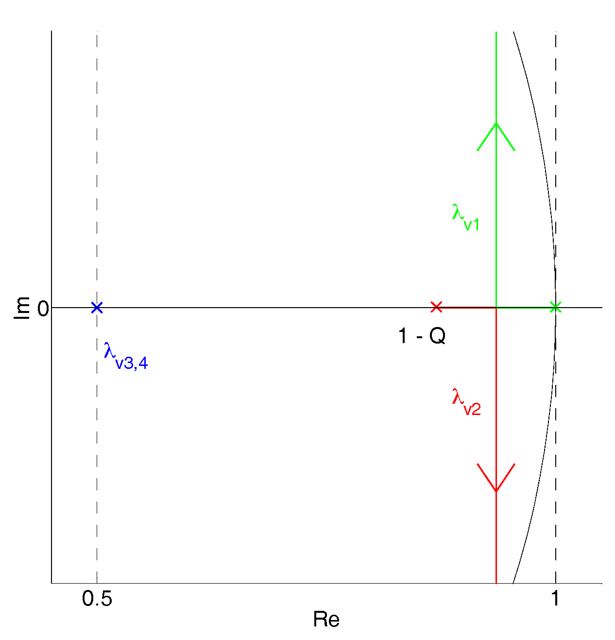
Figure 5 shows the root locus chart of poles with varying parameter $K_p$ from 0 to infinity. Observer poles were expected to be closer to the unit circle origin, so their impact on the system dynamics can be neglected. By setting $K_p=0$ in (49) and comparing it to Equation (21), it can be observed that pole ${\lambda }_{v1}$ originates from the voltage part and pole ${\lambda }_{v2}$ originates from the current part. As $K_p$ is increased, both poles approach each other. For cascade control it is desired that the inner current control loop has higher bandwidth than the outer voltage loop. In other words, the voltage pole must be dominant over the current pole. This is also desired from the emulation perspective, as, with the voltage pole being dominant, reduction of system order is possible. The same rule for pole dominance as in Section 3.3 can also be applied here. From Figure 5 it can be deduced that poles ${\lambda }_{v1}$ and ${\lambda }_{v2}$ must remain on the real axis, and must be far enough apart so that ${\lambda }_{v1}$ stays closer to the unit circle, therefore being dominant. For poles to be real, the range for the control parameter is $K_p\le \frac{Q}{4}$, which can be deduced from (49).

The natural frequency ${\mathsf{\omega }}_{v2}$ of pole ${\lambda }_{v2}$ should be more than five times the natural frequency ${\mathsf{\omega }}_{v1}$ of pole ${\lambda }_{v1}$. This is possible only if both poles are placed on the real axis, and the condition is (50) (similar as for the current part (25)).

$${\mathsf{\omega }}_{v2}>5{\mathsf{\omega }}_{v1}$$

(50)

Inequality (51) is derived by using the same equations as in (24), that is, ${\mathsf{\omega }}_{v1}=\frac{-\ln \left({\lambda }_{v1}\right)}{T}$ and ${\mathsf{\omega }}_{v2}=\frac{-\ln \left({\lambda }_{v2}\right)}{T}$, which are put into (50). By replacing $Q$ with its value, a solution for $K_p$ can be found with numeric methods.

$${\left(1-\frac{Q}{2}+\frac{\sqrt{-Q\left(4K_p-Q\right)}}{2}\right)}^5>\left(1-\frac{Q}{2}-\frac{\sqrt{-Q\left(4K_p-Q\right)}}{2}\right)$$

(51)

The second requirement for tuning $K_p$ is that $i_{L,r}$ is always inside the limits, thus obtaining globally linear behavior without saturation effects. It was also pointed out in a previous study [5] that, due to $i_{L,r}$ saturation, the voltage loop becomes open and possibly unstable. Like in the case of the current control part (27), the incremental voltage change $\Delta v_o\left(k+1\right)$ can be expressed by (52).

$$\Delta v_o\left(k+1\right)=v_o\left(k+1\right)-v_o\left(k\right)$$

(52)

Putting closed loop voltage Equation (39) into (52), using (42), and neglecting disturbance observer estimate error $e_{dv}\left(k\right)\approx 0$ (this is valid, as the observer has a sufficiently higher natural frequency), the worst case of value of $\Delta v_o\left(k+1\right)$, that is, $\Delta V_{o,C},$ is gained in (53). By selecting the appropriate border value of $v_{o,r}$, that is, $V_{o,r}$, and border value of $v_o$, that is, $V_o$, the equation can give the worst case demanded incremental voltage change $\Delta V_{o,C}$ from the controller.

$$\Delta V_{o,C}=K_p{V}_{o,r}-K_p{V}_o$$

(53)

Putting a simplified converter model (37) into (52) and neglecting mismatch $d_v\left(k\right)$, the worst case possible $\Delta v_o\left(k+1\right)$, i.e., $\Delta V_{o,P}$, can be gained in (54). By selecting the appropriate border value of $i_{L,r}$, that is, $I_{L,r}$, and border value of $i_o$, that is, $I_o$, the equation can give the worst case achievable incremental voltage change $\Delta V_{o,P}$. $I_{L,r}$ as well as $I_o$ can be positive when current flows from the converter, emulating a power source, or negative when current flows into the converter, emulating a power drain. It should be noted here that the converter needs to be designed with sufficient margin on the inductor current, i.e., $I_{L,r}>\frac{I_o}{N}>0$ for positive values of $I_o$ or $I_{L,r}<\frac{I_o}{N}<0$ for negative values of $I_o$.

$$\Delta V_{o,P}=\frac{T}{C_o}\left(N{I}_{L,r}\left(k\right)-I_o\left(k\right)\right)$$

(54)

As $\Delta V_{o,C}$ from (53) can be positive (when $V_{o,r}\ge V_o$), or negative (when $V_{o,r}<V_o$), two different cases of requirements are given in (55).

$$\begin{array}{c}a) \Delta V_{o,C}\le \Delta V_{o,P} when V_{o,r}\ge V_o,\\ b) \Delta V_{o,C}\ge \Delta V_{o,P} when V_{o,r}<V_o\end{array}$$

(55)

By using (53) and (54) in (55), two cases of requirements of $K_p$ are gained in (56). Equations for both are similar, only the minimal (min) and maximal (max) worst-case values are different, as they were selected to give the most restrictive worst case.

$$\begin{array}{c}a) K_p\le \frac{1}{V_{o,r,max}-V_{o,min}}\frac{T}{C_o}\left(N{I}_{L,r,max}\left(k\right)-I_{o,max}\left(k\right)\right)\\ b) K_p\le \frac{1}{V_{o,r,min}-V_{o,max}}\frac{T}{C_o}\left(N{I}_{L,r,min}\left(k\right)-I_{o,min}\left(k\right)\right)\end{array}$$

(56)

Equations (51) and (56) are, therefore, the main rules to select parameter $K_p$.

4.2. Voltage Control Model Reduction

The dynamics of the closed voltage loop, current loop and disturbance observer (47) are of the fourth order, which is complex for future use in emulation algorithms. However, in the preceding derivation, it has been assured that the voltage model is dominant over current and observer models. Model reduction is, therefore, possible like in the case of the current controller (Chapter 3.4). SPA can be applied to observer states $e_v\left(k\right)$, $e_{dv}\left(k\right)$ and inductor current $i_L\left(k\right)$ by using (57).

$$\begin{array}{c}{e}_{dv}\left(k+1\right)=e_{dv}\left(k\right)\\ e_v\left(k+1\right)=e_v\left(k\right)\\ i_L\left(k+1\right)=i_L\left(k\right)\end{array}$$

(57)

By using (57) in (47) approximated system states are gained in (58).

$$\begin{array}{c}{e}_v\left(k\right)=e_{dv}\left(k\right)=0\\ i_{L,r}\left(k\right)=\frac{K_p{C}_o}{NT}\left(v_{o,r}\left(k\right)-v_o\left(k\right)\right)+\frac{1}{N}{i}_o\left(k\right)-\frac{C_o}{NT}{d}_v\left(k\right)\end{array}$$

(58)

Putting (58) into the voltage part of (47) ($v_o\left(k+1\right)$), reduced order voltage Equation (59) is obtained.

$$v_o\left(k+1\right)=\left(1-K_p\right)v_o\left(k\right)+K_p{v}_{o,r}\left(k\right)$$

(59)

It is a simple reduced model of the first order, which gives an accurate enough description of the system dynamics. By designing control parameters with the use of the rules presented, they will be globally linear and valid for large signal changes.

5. Results

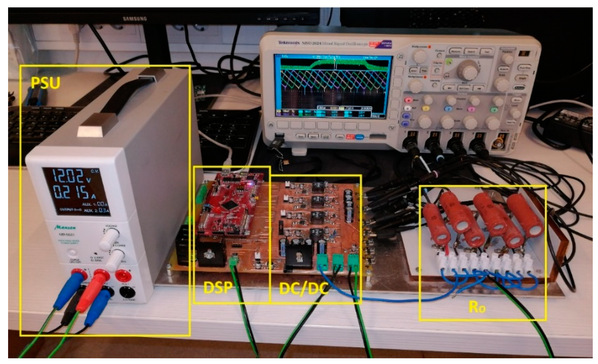
A prototype 4-phase synchronous buck converter was built to prove the concept of the proposed control algorithm. Figure 6 shows the prototype converter and the experimental setup with a power supply unit (PSU) and load ($R_o$). The input voltage ($v_i$) range was from 10 V to 14.4 V, and output voltage ($v_o)$ was from 2 V to 8.5 V. The converter was designed for bidirectional operation, where the output current ranges from −2.5 A to 2.5 A. Load is adjustable by switching different combinations of 12 Ω resistors on-off. Four dual MOSFETs of type FDMS9620 were used for the power part. A3946 was used as a gate driver in all phases, which enabled 0–100 % duty ratio operation. The inductors were MSS1583, with saturation current of 2.0 A (for 10 % inductance drop). In this work, the inductor current range used was from −1.0 A to 1.0 A, so it stayed in the linear region. Input and output voltages ($v_i, v_o$) were sensed; for currents, the current shunts were on all 4 phases for sensing $i_{L1\dots 4},$ and on output for sensing $i_o$. The basic power part component values are presented in

Table 1. Prototype converter parameters.

Parameter	Symbol	Value
Inductor inductances	$L_{1\dots 4}$	330 µH
Inductor resistances	$R_{L,1\dots 4}$	300 mΩ
Input, output capacitance	$C_i, C_o$	1880 µF
Input, output ESR	$ES{R}_{Ci}, ES{R}_{Co}$	20 mΩ
High MOSFETs ($Q_{1,3,5,7})$ on-state resistance	$R_{ds-ON,U}$	21.5 mΩ
Low MOSFETs ($Q_{2,3,6,8})$ on-state resistance	$R_{ds-ON,L}$	13 mΩ
Current sense shunt resistances	$R_{cs}$	3 Ω

. A Texas Instruments DSP, TMS320F28377S, was used to implement the control algorithm. The control algorithm and PWM executed with 20 kHz, where the same algorithm was applied for each phase current control, and one master algorithm was applied for voltage control. PWM pulses were synchronized and delayed by 90° from each other. Center aligned PWM sampling was used for phase currents, so average current values were obtained for a defined period.

5.1. Sliding Mode Current Control with a Disturbance Observer

By using SMC, system dependence on nominal circuit parameters was canceled; any parameter deviations and sensor errors are included in disturbance estimate ${\widehat{d}}_i\left(k\right)$ from the observer. Using the proposed tuning rules, system stability can be gained in a global sense and operating point independent dynamics.

Table 2. Current subsystem marginal values.

Variable	Value
$I_{L,r,min}$, $I_{L,min}$	−1 A
$I_{L,r,max}$, $I_{L,max}$	1 A
$V_{i,min}$	10 V
$V_{i,max}$	14.4 V
$V_{o,min}$	2 V
$V_{o,max}$	8.5 V
$U_{min}$	0
$U_{max}$	1

contains selected system marginal variables, which were used in (31) together with the parameters from Table 1, to gain two conditions ($Q<0.14$ and $Q<0.18$) for the algorithm to operate always inside the saturation limits. The third condition for parameter $Q$ ($Q\le 0.13)$ is given in (26). Based on that, control parameter $Q=0.13$ was selected, which gives the fastest system response. Observer gain $l_i$ was selected in (22) and is independent of system parameters. By using $Q,l_i,$ and system parameters, the control law (10) and the disturbance observer (12), (13) were implemented on DSP in the control algorithm of each phase. All tests were performed at a constant input voltage $V_i=12 V$.

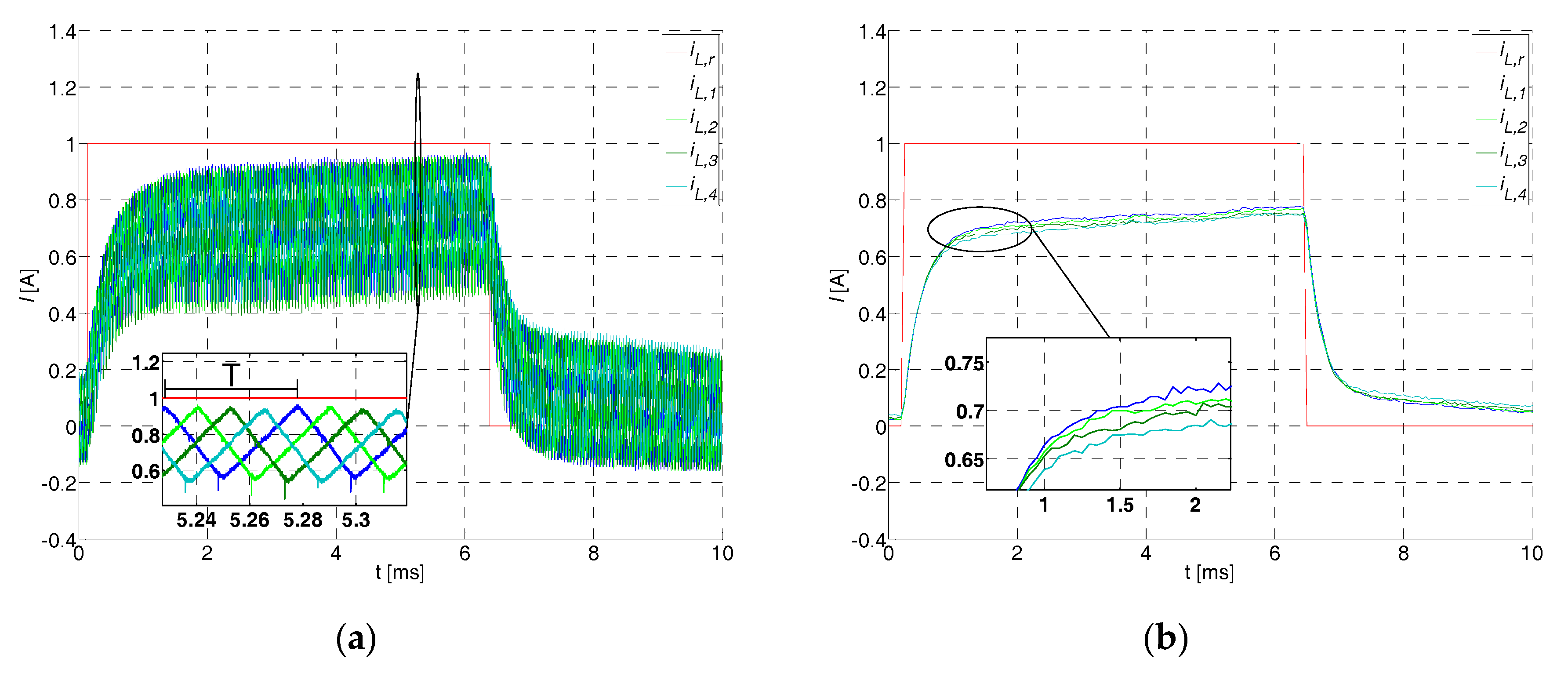
The operation of the converter was first checked for current control only. The load was ohmic resistance $R_o=3 \Omega ,$ and the current reference $i_{L,r}$ was varied from 0 to 1 A. The period of reference value was set to 10 ms; this way, the output voltage was in the operational range (as the voltage control loop was opened, the voltage could rise up to its limits). In order to present the benefits of using SMC with Disturbance Observer (DO), operation of SMC was first investigated based on a nominal model. This can be accomplished by using control law (10) without disturbance estimate, that is, ${\widehat{d}}_{i,n}\left(k\right)=0$. The responses of phase currents are shown in Figure 7a. Figure 7b shows the values of currents, sampled by DSP, which were used in the control algorithm. It can be observed that reference tracking was poor and currents were not equal. This is because of model imperfections which were not compensated for.

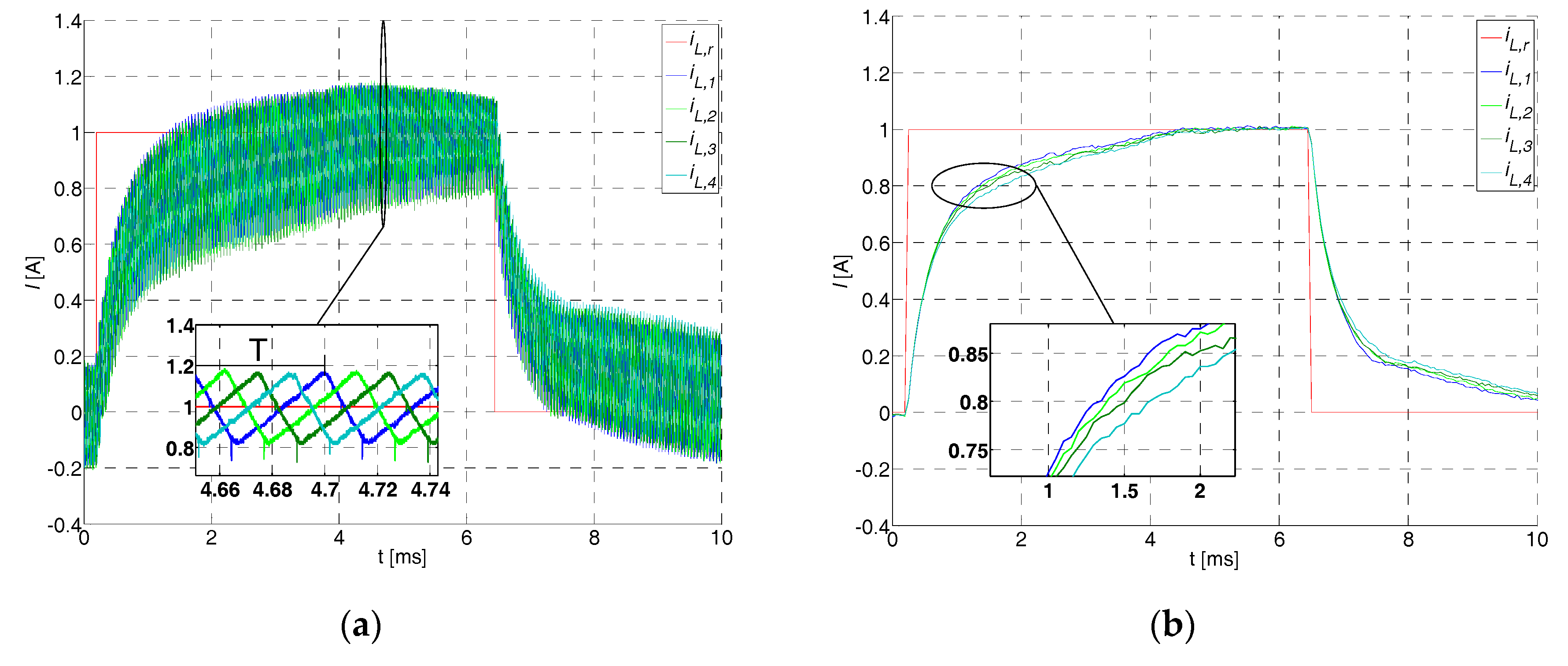
Then, the control performance was checked for the well-known integral sliding mode (ISM). This can be accomplished by using the additional integrative state in (10), and setting ${\widehat{d}}_{i,n}\left(k\right)=0$. Figure 8a shows current responses; compared to the previous case, the currents reached the current reference, that is, model imperfections were compensated for. Figure 8b shows current values, sampled by DSP, and it can be seen that, while reaching the current reference, currents were unbalanced. During that phase, the integral part of ISM was in operation, its dynamics were added to the system’s and it can be observed from the response.

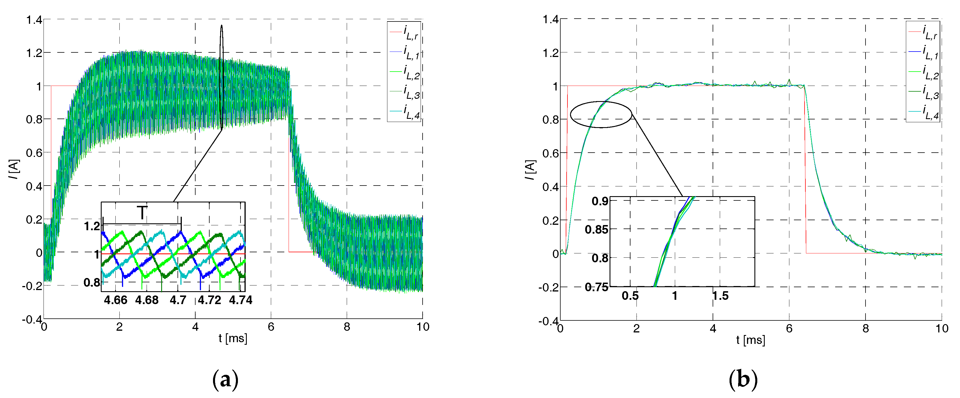
Then, the operation of the SMC algorithm was verified with the disturbance observer, according to (10). Figure 9a shows the current responses, which reached reference faster than in previous examples (Figure 7 and Figure 8). Figure 9b shows the sampled currents, where good tracking of reference can be observed. Compared to previous cases, currents were balanced, even while reaching the reference; this is convenient, as their dynamical description is the same, as well as from the electronic circuit perspective, because better current distribution and equal heating of phases was accomplished.

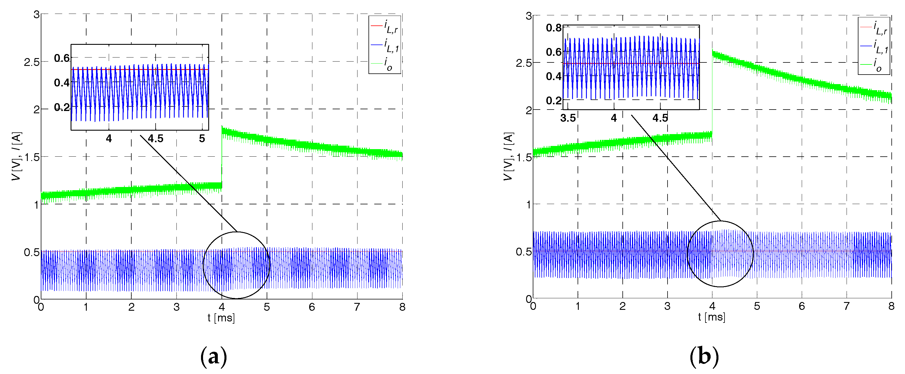
Next, response to load change was observed, with $i_{L,r}=0.5A$ and $R_o$ changed from 3 Ω to 2 Ω.

Figure 10 shows the results, where the output current step and output voltage can be seen, the latter being inside the operational range of the converter. Output load change does not affect controller performance significantly for non-observer or observer cases, although, by using the observer, current value is recovered to value before the load change.

5.2. Voltage Control and Disturbance Observer

As in the current control, system dependence on nominal parameters was canceled by the proposed control law; any parameter deviations and sensor errors were included in the disturbance estimate ${\widehat{d}}_v\left(k\right)$. By following the proposed tuning rules, a globally stable system could be gained with operating point independent dynamics.

Table 3. Voltage subsystem marginal values.

Variable	Value
$V_{o,min}$, $V_{o,r,min}$	2 V
$V_{o,max}$, $V_{o,r,max}$	8.5 V
$I_{L,r,min}$	−1 A
$I_{L,r,max}$	1 A
$I_{L,r,max}$, $I_{L,max}$	1 A
$I_{o,min}$	−2.5 A
$I_{o,max}$	2.5 A

contains the marginal values of system variables, which were used in (56), together with the parameters from Table 1, in order to obtain the value of parameter $K_p,$ which will assure us that the algorithm always operates inside the inductor current marginal values, that is, $K_p\le 0.00614$ for both cases. Equation (51) gives the second condition for the choice of $K_p,$ with the use of $Q$ applied in the current control design. The value used was $K_p=0.006$. By using this value and system parameters, control law (38) with disturbance observers (40) and (41), could be implemented on DSP. The result from (38) was then used as a reference for all phase current control loops. It can easily be compared to a P controller with output current feedforward control, which was accomplished by setting ${\widehat{d}}_v\left(k\right)=0$ in (38). By using integral of voltage error instead of ${\widehat{d}}_v\left(k\right)$, the well-known PI controller could be implemented with output current feedforward.

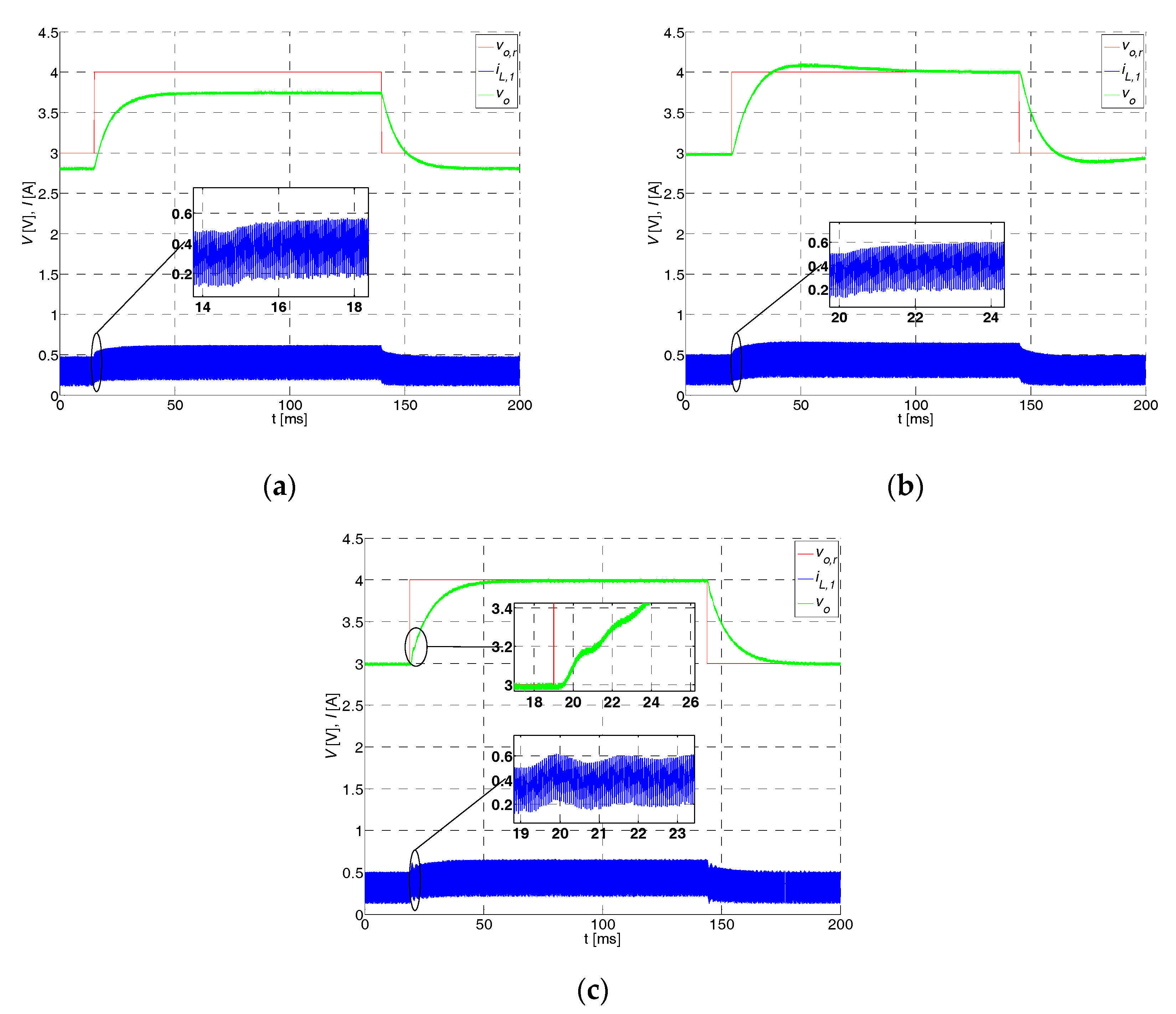
The operation of all controllers was verified by reference voltage steps from 3 V to 4 V, with the $R_o=2 \Omega$. Figure 11a shows the operation for output current feedforward, combined with a P-type controller. A stationary error can be observed, which was the result of model imperfection, sensor errors, and so on. Figure 11b shows the improved version (PI controller with output current feedforward). As can be seen, stationary state error has been removed, although, some additional system dynamics can be observed in the form of overshoot. Figure 11c shows the operation of output current feedforward combined with the disturbance observer, which was derived in the current work. The results controller removes the stationary error as with the controller in Figure 11b, but, without additional dynamics, there was no overshoot. This could be accomplished as the observer was active only for model imperfections, compared with the integral part of PI, which was active all the time, resulting in overshoots, control signal saturation and long settling times. The observer dynamics are magnified in Figure 11c; by using the proposed tuning rules it was made negligible.

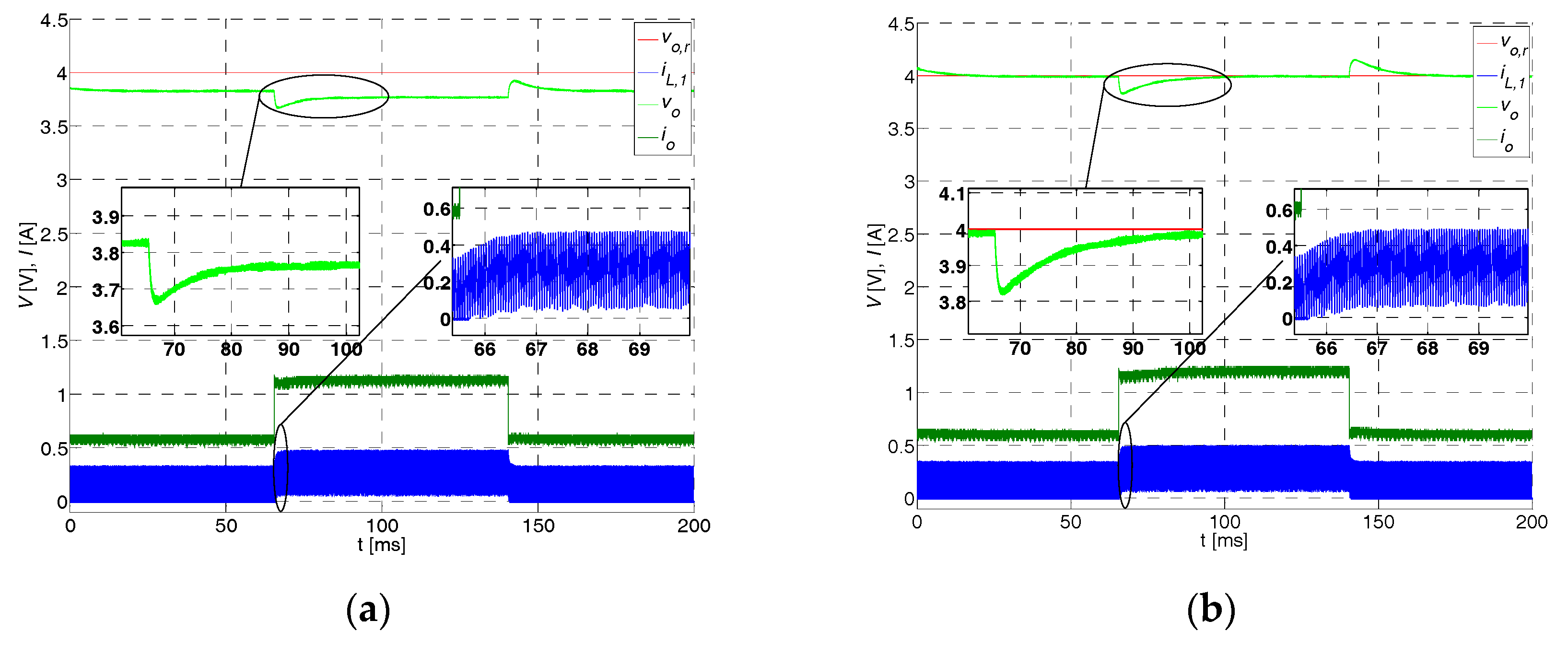
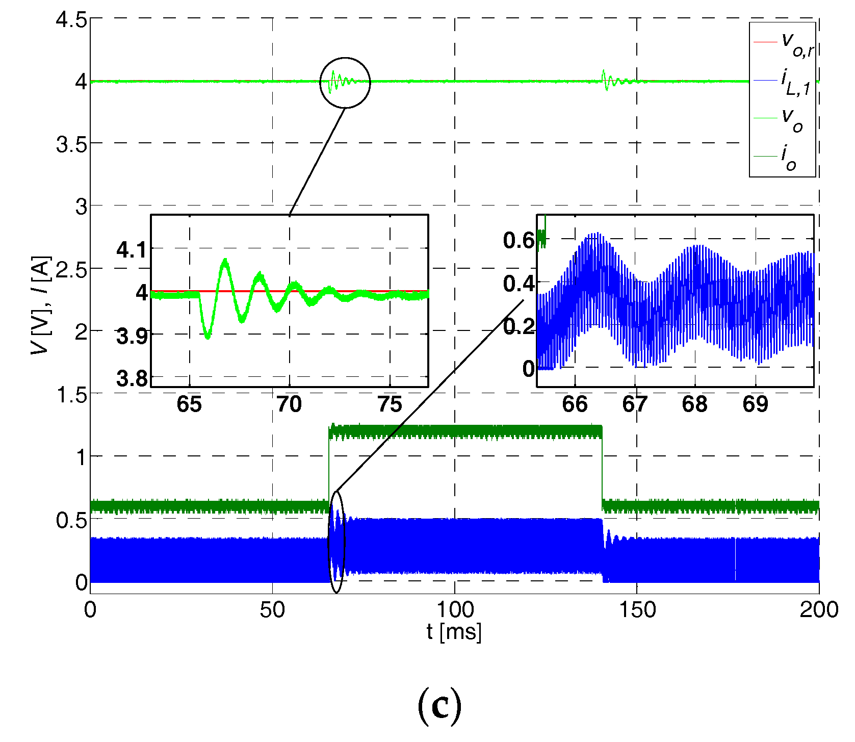
Next, the operation of all three controllers was checked in response to load step. Voltage reference was set to 4 V and the load $R_o$ was changed from $6 \Omega$ to $3 \Omega$ and back. The results in Figure 12a show that there was some stationary error in the operation of the P type controller with $i_o$ feedforward, which was the result of an unmatched model. Figure 12b shows improvement when using a PI controller with $i_o$ feedforward, as the stationary error was reduced. Figure 12c shows the operation of a P controller with $i_o$ feedforward and disturbance observer. Stationary state error was reduced, as in the case of PI, but settling is much faster. There were some oscillations in inductor current and output voltage. They can be explained by Figure 5, where they appear as observer poles which have been placed in the marginal point before becoming complex values. The model of the converter is not perfect; some simplifications were applied in (36) and (37), where one sample time delay was neglected, and this could explain the oscillations. Oscillations could be eliminated by manually tuning parameter $l_v$ to a lower value, but it is not necessary, as their amplitude is low. The contribution of this work is to show that observer poles can be placed analytically, and that they are not dominant in voltage response.

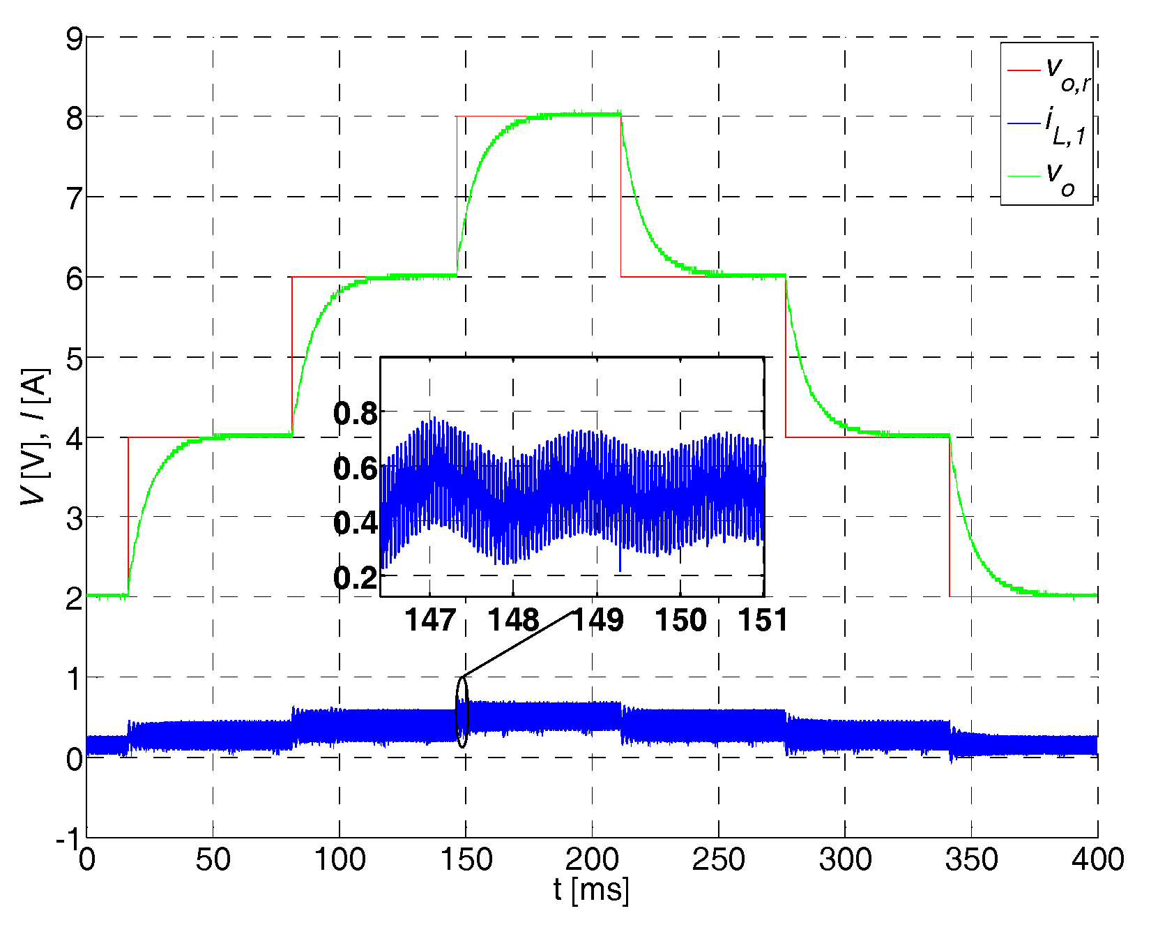
Operation in the whole operational range of output voltage was checked by different voltage reference steps between 2 V, 4 V, 6 V and 8 V, with $R_o=4\Omega$. Figure 13 shows the results, where voltage responses can be regarded as the same for all operating points. It can be assumed from phase 1 current $i_{L1}$ that it is inside the designed bounds presented in Table 3. The oscillations in the current are not problematic, as its value remains well below $I_{L,max}$ (this can be assumed since for $V_o=8\mathrm{V}$, and $R_o=4\Omega$ the output current is 2 A, which is close to the maximum rated load). As already mentioned before, they can be eliminated by tuning $l_v\mathrm{manually}$ if necessary.

6. Discussion

A control algorithm has been proposed for control of a multiphase buck converter. Inner control sliding surfaces take care of current control for each phase, and make the current loops’ model linear and operating points independent. The saturation of duty ratio is prevented with the proposed tuning rules. Model imperfections in the form of discretization errors, dead time effects, and parameter uncertainties, have been compensated for by the introduction of disturbance observers. Compared to ISM [34], a disturbance observer is active only when model imperfections exist, and it alters the system dynamics minimally. When model imperfections are present, observer dynamics are non-dominant if the proposed tuning rules are followed. Parameters are determined analytically. Compared to ISM, a disturbance observer does not suffer from wind-up effects, as the estimated disturbance value is bounded. Its maximum value could be calculated based on predicted model imperfections with some additional analysis, but this has been omitted in the present work to simplify the design. Another benefit of a disturbance observer over the ISM is phase currents are equal while reaching current reference, resulting in equal dynamics and better heating distribution in a circuit. Control signal limiting is not needed with the use of the proposed tuning rules, resulting in a globally linear model. For the voltage part control, a disturbance observer of the same structure has been used, and the same rules can be used for tuning, which simplifies the design. Although disturbance in the voltage part is mismatched, it has been shown that it can be compensated for sufficiently by current loops tuned to a higher bandwidth than the voltage loop. By evaluating the estimated disturbance value, it would be possible also to evaluate model accuracy. If necessary, accuracy can be improved with model expansion by introduction of additional parameters, like output capacitance, equivalent series resistance (ESR), dead times, or use of discretization of higher orders, and so on.

It was confirmed that the proposed algorithm makes the converter characteristic linear and operating points independent. Voltage responses were identical in the whole output voltage range, which is convenient in later use for emulation of batteries in a wide range of voltages. Compared to the PI voltage control with the output current feedforward, there were no additional dynamics, which would manifest in form of overshoots. Model reduction based on SPA was applied to gain a simple closed loop description of the converter without nonlinear effects, which can be used later by the battery emulation algorithm. It was confirmed that the control algorithm can be implemented on a DSP, unlike MPC [8,31], which is computationally more complex, needing more powerful processors. Controller delay because of sample and hold operation was neglected in this work, as the switching frequency was sufficiently higher than the controller bandwidth. If needed, its effects can be analyzed and compensated for in future work.

References

- Mousavi, G.S.M.; Nikdel, M. Various battery models for various simulation studies and applications. Renew. Sustain. Energy Rev. 2014, 32, 477–485. [Google Scholar] [CrossRef]
- Rivetta, C.; Williamson, G.A. Large-signal analysis and control of buck converters loaded by DC-DC converters. In Proceedings of the 2004 IEEE 35th Annual Power Electronics Specialists Conference (IEEE Cat. No.04CH37551), Aachen, Germany, 20–25 June 2004; Volume 3675, pp. 3675–3680. [Google Scholar]
- Qiu, W.; Mercer, S.; Liang, Z.; Miller, G. Driver deadtime control and its impact on system stability of synchronous buck voltage regulator. IEEE Trans. Power Electron. 2008, 23, 163–171. [Google Scholar] [CrossRef]
- Emadi, A.; Khaligh, A.; Rivetta, C.H.; Williamson, G.A. Constant power loads and negative impedance instability in automotive systems: definition, modeling, stability, and control of power electronic converters and motor drives. IEEE Trans. Veh. Technol. 2006, 55, 1112–1125. [Google Scholar] [CrossRef]
- El Aroudi, A.; Martínez-Treviño, B.A.; Vidal-Idiarte, E.; Cid-Pastor, A. Fixed switching frequency digital sliding-mode control of DC-DC power supplies loaded by constant power loads with inrush current limitation capability. Energies 2019, 12, 1055. [Google Scholar] [CrossRef]
- König, O.; Hametner, C.; Prochart, G.; Jakubek, S. Battery Emulation for Power-HIL Using Local Model Networks and Robust Impedance Control. IEEE Trans. Ind. Electron. 2014, 61, 943–955. [Google Scholar] [CrossRef]
- Karimi, R.; Kaczorowski, D.; Zlotnik, A.; Mertens, A. Loss optimizing control of a multiphase interleaving DC-DC converter for use in a hybrid electric vehicle drivetrain. In Proceedings of the 2016 IEEE Energy Conversion Congress and Exposition (ECCE), Milwaukee, WI, USA, 18–22 September 2016; pp. 1–8. [Google Scholar]
- König, O.; Gregorčič, G.; Jakubek, S. Model predictive control of a DC–DC converter for battery emulation. Control Eng. Pract. 2013, 21, 428–440. [Google Scholar] [CrossRef]
- König, O.; Jakubek, S.; Prochart, G. Battery impedance emulation for hybrid and electric powertrain testing. In Proceedings of the 2012 IEEE Vehicle Power and Propulsion Conference, Seoul, Korea, 9–12 October 2012; pp. 627–632. [Google Scholar]
- Rodič, M.; Milanovič, M.; Truntič, M. Digital control of an interleaving operated buck-boost synchronous converter used in a low-cost testing system for an automotive powertrain. Energies 2018, 11, 2290. [Google Scholar] [CrossRef]
- Eirea, G.; Sanders, S.R. Phase current unbalance estimation in multiphase buck converters. IEEE Trans. Power Electron. 2008, 23, 137–143. [Google Scholar] [CrossRef]
- Mariethoz, S.; Beccuti, A.G.; Morari, M. Model predictive control of multiphase interleaved DC-DC converters with sensorless current limitation and power balance. In Proceedings of the 2008 IEEE Power Electronics Specialists Conference, Rhodes, Greece, 15–19 June 2008; pp. 1069–1074. [Google Scholar]
- Schumacher, D.; Magne, P.; Preindl, M.; Bilgin, B.; Emadi, A. Closed loop control of a six phase interleaved bidirectional dc-dc boost converter for an EV/HEV application. In Proceedings of the 2016 IEEE Transportation Electrification Conference and Expo (ITEC), Dearborn, MI, USA, 27–29 June 2016; pp. 1–7. [Google Scholar]
- Ou, S.Y.; Liu, L.Y. Design and implementation of a four-phase converter with digital current sharing control for battery charger. In Proceedings of the 2015 IEEE International Telecommunications Energy Conference (INTELEC), Osaka, Japan, 18–22 October 2015; pp. 1–6. [Google Scholar]
- Yang, Q.; Juanjuan, S.; Ming, X.; Kisun, L.; Lee, F.C. High-bandwidth designs for voltage regulators with peak-current control. In Proceedings of the Twenty-First Annual IEEE Applied Power Electronics Conference and Exposition, APEC ‘06, Dallas, TX, USA, 19–23 March 2006; p. 7. [Google Scholar]
- Ridley, R.B. A New Small-Signal Model for Current-Mode Control; Virginia Polytechnic Institute and State University: Blacksburg, VA, USA, 1999. [Google Scholar]
- Truntič, M.; Milanovič, M. Voltage and current-mode control for a buck-converter based on measured integral values of voltage and current implemented in FPGA. IEEE Trans. Power Electron. 2014, 29, 6686–6699. [Google Scholar] [CrossRef]
- Cooke, P. Modeling average current mode control. In Proceedings of the APEC 2000—Fifteenth Annual IEEE Applied Power Electronics Conference and Exposition (Cat. No.00CH37058), New Orleans, LA, USA, 6–10 February 2000; Volume 251, pp. 256–262. [Google Scholar]
- Han, J. From PID to active disturbance rejection control. IEEE Trans. Ind. Electron. 2009, 56, 900–906. [Google Scholar] [CrossRef]
- Szeifert, F.; Nagy, L.; Chován, T.; Abonyi, J. Constrained PI(D) algorithms (C-PID). Hungarian J. Ind. Chem. 2005, 33, 81–88. [Google Scholar]
- Halihal, Y. State-Space Oriented Advanced Analysis And Control Mehtods of Switching Converters; Ben-Gurion University of the Negev: Beersheba, Israel, 2015. [Google Scholar]
- Repecho, V.; Biel, D.; Ramos-Lara, R.; Vega, P.G. Fixed-switching frequency interleaved sliding mode eight-phase synchronous buck converter. IEEE Trans. Power Electron. 2018, 33, 676–688. [Google Scholar] [CrossRef]
- Repecho, V.; Biel, D.; Ramos, R.; Garcia, P. Sliding mode control of a m-phase DC/DC buck converter with chattering reduction and switching frequency regulation. In Proceedings of the 2016 14th International Workshop on Variable Structure Systems (VSS), Nanjing, China, 1–4 June 2016; pp. 290–295. [Google Scholar]
- Lopez, M.; Vicuna, L.G.D.; Castilla, M.; Lopez, O.; Majo, J. Interleaving of parallel DC-DC converters using sliding mode control. In Proceedings of the IECON ‘98 24th Annual Conference of the IEEE Industrial Electronics Society (Cat. No.98CH36200), Aachen, Germany, 31 August–4 September 1998; Volume 1052, pp. 1055–1059. [Google Scholar]
- Mazumder, S.K. Nonlinear Analysis and Control of Standalone, Parallel DC-DC, and Parallel Multi-Phase PWM Converters; Faculty of the Virginia Polytechnic Institute and State University: Blacksburg, VA, USA, 2001. [Google Scholar]
- Zongxiang, C.; Ya-nan, G.; Mingxing, C.; Lusheng, G. Study on PI sliding mode controller for paralleled dc-dc converter. In Proceedings of the 2016 IEEE 8th International Power Electronics and Motion Control Conference (IPEMC-ECCE Asia), Hefei, China, 22–26 May 2016; pp. 3079–3083. [Google Scholar]
- Marcos-Pastor, A.; Vidal-Idiarte, E.; Cid-Pastor, A.; Martinez-Salamero, L. Interleaved digital power factor correction based on the sliding-mode approach. IEEE Trans. Power Electron. 2016, 31, 4641–4653. [Google Scholar] [CrossRef]
- Vidal-Idiarte, E.; Marcos-Pastor, A.; Giral, R.; Calvente, J.; Martinez-Salamero, L. Direct digital design of a sliding mode-based control of a PWM synchronous buck converter. IET Power Electron. 2017, 10, 1714–1720. [Google Scholar] [CrossRef]
- Weibing, G.; Yufu, W.; Homaifa, A. Discrete-time variable structure control systems. IEEE Trans. Ind. Electron. 1995, 42, 117–122. [Google Scholar] [CrossRef]
- Monses, G. Discrete-Time Sliding Mode Control; Technische Universiteit Delft: Delft, The Netherlands, 2002. [Google Scholar]
- König, O.; Jakubek, S.; Prochart, G. Model predictive control of a battery emulator for testing of hybrid and electric powertrains. In Proceedings of the 2011 IEEE Vehicle Power and Propulsion Conference, Chicago, IL, USA, 6–9 September 2011; pp. 1–6. [Google Scholar]
- Orosco, R.; Vazquez, N. Discrete sliding mode control for DC/DC converters. In Proceedings of the 7th IEEE International Power Electronics Congress, Technical Proceedings, CIEP 2000 (Cat. No.00TH8529), Acapulco, Mexico, 15–19 October 2000; pp. 231–236. [Google Scholar]
- Cao, J.; Chen, Q.; Zhang, L.; Quan, S. Sliding mode control of bidirectional DC/DC converter. In Proceedings of the 2018 33rd Youth Academic Annual Conference of Chinese Association of Automation (YAC), Atlanta, GA, USA, 18–20 May 2018; pp. 717–721. [Google Scholar]
- Abidi, K.; Jian-Xin, X. A Discrete-Time Integral Sliding Mode Control Approach for Output Tracking with State Estimation. IFAC Proc. Vol. 2008, 41, 14199–14204. [Google Scholar] [CrossRef] [Green Version]
- Zheng, C.; Zhang, J. Finite-time nonlinear disturbance observer based discretized integral sliding mode control for PMSM drives. J. Power Electron. 2018, 18, 1075–1085. [Google Scholar] [CrossRef]
- Yang, J.; Li, S.; Yu, X. Sliding-mode control for systems with mismatched uncertainties via a disturbance observer. IEEE Trans. Ind. Electron. 2013, 60, 160–169. [Google Scholar] [CrossRef]
- Yang, J.; Su, J.; Li, S.; Yu, X. High-order mismatched disturbance compensation for motion control systems via a continuous dynamic sliding-mode approach. IEEE Trans. Ind. Inf. 2014, 10, 604–614. [Google Scholar] [CrossRef]
- Yin, Y.; Liu, J.; Vazquez, S.; Wu, L.; Franquelo, L.G. Disturbance observer based second order sliding mode control for DC-DC buck converters. In Proceedings of the IECON 2017—43rd Annual Conference of the IEEE Industrial Electronics Society, Beijing, China, 29 October–1 November 2017; pp. 7117–7122. [Google Scholar]
- Wang, J.; Li, S.; Yang, J.; Wu, B.; Li, Q. Finite-time disturbance observer based non-singular terminal sliding-mode control for pulse width modulation based DC–DC buck converters with mismatched load disturbances. IET Power Electron. 2016, 9, 1995–2002. [Google Scholar] [CrossRef]
- Sanjeev Kumar, P.; Patil, S.L.; Chaudhari, B.N. Disturbance observer based sliding mode control for DC-DC power converters. In Proceedings of the IECON 2016—42nd Annual Conference of the IEEE Industrial Electronics Society, Florence, Italy, 23–26 October 2016; pp. 3366–3371. [Google Scholar]
- Pandey, S.K.; Patil, S.L.; Chaskar, U.M.; Phadke, S.B. Direct Duty Ratio Control of Buck DC-DC Converters Using Disturbance Observer Based Integral Sliding Mode Control. In Proceedings of the IECON 2018—44th Annual Conference of the IEEE Industrial Electronics Society, Washington, DC, USA, 21–23 October 2018; pp. 5507–5512. [Google Scholar]
- Kim, K.-S.; Rew, K.-H. Reduced order disturbance observer for discrete-time linear systems. Automatica 2013, 49, 968–975. [Google Scholar] [CrossRef]
- Maksimovic, D.; Zane, R. Small-signal Discrete-time Modeling of Digitally Controlled DC-DC Converters. In Proceedings of the 2006 IEEE Workshops on Computers in Power Electronics, Troy, NY, USA, 16–19 July 2006; pp. 231–235. [Google Scholar]
- Feng, C.; Lin, Y. Robust control design based-on integral sliding-mode for systems with norm-bounded uncertainties. In Proceedings of the 2011 11th International Conference on Control, Automation and Systems, Gyeonggi-do, Korea, 26–29 October 2011; pp. 1178–1183. [Google Scholar]
- Siew-Chong, T.; Yuk-Ming, L.; Chi Kong, T. Sliding Mode Control of Switching Power Converters; Taylor & Francis Group, LLC: New York, NY, USA, 2012. [Google Scholar]
- Xiong, L.; Li, P.; Li, H.; Wang, J. Sliding mode control of DFIG wind turbines with a fast exponential reaching law. Energies 2017, 10, 1788. [Google Scholar] [CrossRef]
- Yang, Z.; Wan, L.; Sun, X.; Li, F.; Chen, L. sliding mode variable structure control of a bearingless induction motor based on a novel reaching law. Energies 2016, 9, 452. [Google Scholar] [CrossRef]
- Bartoszewicz, A.; Leśniewski, P. Refined reaching laws for sliding mode control of discrete time systems. In Proceedings of the 2013 18th International Conference on Methods & Models in Automation & Robotics (MMAR), Miedzyzdroje, Poland, 26–29 August 2013; pp. 824–829. [Google Scholar]
- Lee, C.W.; Chung, C.C. An approach to discrete-time sliding mode control with variable convergence rate to sliding surface. In Proceedings of the 2008 SICE Annual Conference, Tokyo, Japan, 20–22 August 2008; pp. 2358–2363. [Google Scholar]
- Bartoszewicz, A.; Leśniewski, P. New Switching and Nonswitching Type Reaching Laws for SMC of Discrete Time Systems. IEEE Trans. Control Syst. Technol. 2016, 24, 670–677. [Google Scholar] [CrossRef]
- Wen-Hua, C. Disturbance observer based control for nonlinear systems. IEEE/ASME Trans. Mechatron. 2004, 9, 706–710. [Google Scholar] [CrossRef]
- Kaiwei, Y.; Yuancheng, R.; Lee, F.C. Critical bandwidth for the load transient response of voltage regulator modules. IEEE Trans. Power Electron. 2004, 19, 1454–1461. [Google Scholar] [CrossRef]
- Pit-Leong, W.; Lee, F.C.; Peng, X.; Kaiwei, Y. Critical inductance in voltage regulator modules. IEEE Trans. Power Electron. 2002, 17, 485–492. [Google Scholar] [CrossRef]
- Rydel, M.; Stanisławski, R.; Latawiec, K.J.; Gałek, M. Model order reduction of commensurate linear discrete-time fractional-order systems. IFAC-PapersOnLine 2018, 51, 536–541. [Google Scholar] [CrossRef]
Figure 1.
Multiphase synchronous DC-DC converter.
Figure 2.
Diagram of sliding mode control (SMC) and disturbance observer for phase current control.
Figure 3.
Root-locus chart for the SCM pole and observer poles .
Figure 4.
A diagram of voltage control, disturbance observer and N-inner current control loops. Proposed rules to tune the output voltage controller.
Figure 5.
Root-locus chart for voltage control poles and disturbance observer poles
Figure 6.
Test setup for prototype converter with ohmic load.
Figure 7.
Phase currents’ responses to step change of current reference from 0 to 1 A when SMC is used, based on a nominal model without uncertainties; (a) real current values and (b) current values, sampled by digital signal processor (DSP).
Figure 8.
Phase currents’ responses to step change of current reference from 0 to 1 A when integral sliding mode (ISM) is used to account model uncertainties; (a) real current values and (b) values, sampled by DSP.
Figure 9.
Phase currents’ to step change of current reference from 0 to 1 A when a disturbance observer is used to account for model uncertainties; (a) real current values and (b) values, sampled by DSP.
Figure 10.
Phase 1 current response with reference current = 0.5 A and load change from 3 Ω to 2 Ω without observer (a) and with observer (b).
Figure 11.
Output voltage response to step voltage reference change when using (a) P type control with feedforward, (b) PI control with feedforward, and (c) P control with feedforward and disturbance observer. The load was 2 Ω.
Figure 12.
Output voltage and phase 1 current response to load change from 6 Ω to 3 Ω and back when using (a) P type control with feedforward, (b) PI control with feedforward, (c) P control with feedforward and disturbance observer.
Figure 13.
Output voltage and phase 1 current response to 2 V reference voltage steps in the whole operating range.