On Wind Turbine Loads During Thunderstorm Downbursts in Contrasting Atmospheric Stability Regimes


1
Department of Civil, Architectural and Environmental Engineering, The University of Texas at Austin, Austin, TX 78712, USA
2
Department of Marine, Earth, and Atmospheric Sciences, North Carolina State University, Raleigh, NC 27695, USA
3
Faculty of Civil Engineering and Geosciences, Delft University of Technology, 2628 CN Delft, The Netherlands
*
Author to whom correspondence should be addressed.
Energies 2019, 12(14), 2773; https://doi.org/10.3390/en12142773
Submission received: 24 June 2019
/
Revised: 13 July 2019
/
Accepted: 16 July 2019
/
Published: 19 July 2019
(This article belongs to the Section A3: Wind, Wave and Tidal Energy)
Abstract
:Severe winds produced by thunderstorm downbursts pose a serious risk to the structural integrity of wind turbines. However, guidelines for wind turbine design (such as the International Electrotechnical Commission Standard, IEC 61400-1) do not describe the key physical characteristics of such events realistically. In this study, a large-eddy simulation model is employed to generate several idealized downburst events during contrasting atmospheric stability conditions that range from convective through neutral to stable. Wind and turbulence fields generated from this dataset are then used as inflow for a 5-MW land-based wind turbine model; associated turbine loads are estimated and compared for the different inflow conditions. We first discuss time-varying characteristics of the turbine-scale flow fields during the downbursts; next, we investigate the relationship between the velocity time series and turbine loads as well as the influence and effectiveness of turbine control systems (for blade pitch and nacelle yaw). Finally, a statistical analysis is conducted to assess the distinct influences of the contrasting stability regimes on extreme and fatigue loads on the wind turbine.
1. Introduction
Thunderstorm downbursts occur as downward momentum generated by hydrometeor drag and latent cooling reach the surface and spread out laterally to create complex and radially divergent horizontal winds [1]. These events are capable of producing severe wind speeds (~26 m/s or greater) and have been known to cause both economic and life-threatening impacts, such as in the destruction of buildings [2] and fatal aviation accidents [3,4]. Furthermore, it has been seen that the outflow winds are capable of producing intense loading on wind turbines and can result in damage or destruction of individual turbines, as was seen at the Buffalo Ridge Wind Farm in 2011 [5]. Thus, it is important to study the effects of downburst winds on contemporary wind turbines in order to improve turbine design and refine control strategies during such extreme events.
In the International Electrotechnical Commission (IEC) guidelines for wind turbine design [6], suggested approaches for the inflow generation are too simplistic to account for the realistic dynamics and physics of downburst winds. Within these guidelines, extreme wind events are represented, for example, by a simple sinusoidal function for wind speed to be applied over a specified fixed duration, with stochastically generated turbulence added on to a mean flow field. From the IEC standard, the extreme operating gust (EOG) is defined as:
where represents the wind speed as a function of height, z, and time, t; is a power-law wind profile; is the gust magnitude at hub height; and T is a specific time span for the gust function, taken to be 10.5 s. These mean wind fields derived from the analytical functions can be grossly different from what has been observed during downbursts [7]; they also may not accurately describe the strong vertical shear observed sometimes, and the associated non-stationary characteristics of the flow field. As well, the turbulence models employed are often for overly simplified cases with assumptions of near-neutral stability conditions that may not be justified. Due to these shortcomings, a series of earlier studies [8,9,10,11,12,13] were conducted to assess how downburst-related inflow fields (based on observational data but analytically derived [14]) could influence turbine loads. These studies highlighted the potential impacts of downbursts on a single wind turbine as well as on an entire wind farm or turbine array. They also emphasized the importance of improved models over the current IEC guidelines suggested for such events, when considering turbine design and control. In comparison with the turbine loads resulting from the IEC load cases for extreme coherent gust (ECG), extreme direction change (EDC), and extreme coherent gust with direction change (ECD), all believed to represent transient events such as downbursts, the turbine loads that were produced when driven by the data-based analytical models differed greatly. (In two cases, as found by Nguyen et al. [8], the analytical models predicted loads that were 86% larger than those based on the IEC EDC load case and 20% larger than those based on the IEC ECD case.) The availability and effectiveness of yaw and pitch control were found to have a significant influence on the resulting turbine loads. These analytical models for downbursts are extremely efficient and are widely applied in wind engineering research for buildings [15], in aviation-related studies [16,17], and in the assessment of turbine loads. Even though these analytical models for the mean wind field and associated turbulence fields are an improvement over the current IEC guidelines, the models are deficient in accurately capturing several physical aspects of the downburst wind fields such as the formation of surface ring vortices [1,18,19,20], spatially coherent structures at the leading edge of a moving downburst [21,22], and accurate representations of the generated turbulence.
In recent years, the modeling of downburst wind fields with the help of large-eddy simulation (LES) has gained in interest. Studies have ranged from those relying on idealized simulations [23,24,25,26,27] to full-storm physics simulations [28,29]. The full-storm simulations have been shown to have the ability to produce realistic high-fidelity data for downburst winds; however, the complex interactions of the microphysics on the resulting simulated storm and wind field produce a convoluted structure, from which direct relationships between cause and effect are generally difficult to assess. Moreover, the computational costs of such simulations are very high since the full-storm simulations require a domain size on the order of 100 of km in the horizontal direction and 10 km in the vertical direction [28,30]; for turbine load modeling, we need a resolution of (10 m) [31], which means that the full-storm simulations may not be feasible. On the other hand, the idealized simulations that use, say, a cooling source approach [23,24] are simplified in that cooling due to the microphysics processes is parameterized as a heat sink; yet, it is still possible to generate high-fidelity datasets that compare favorably with observations. Additionally, the use of the cooling source approach, originally proposed by Anderson et al. [32] allows for much more control of the downburst intensity and location. This approach also does not require the full storm to be resolved; thus, the domain size requirements can be reduced significantly (to the order of a few km) to limit the computational burden of each simulation. Such LES-generated wind fields have been found to describe the principal physical characteristics of downbursts [33] that the analytical models, as previously mentioned, are unable to capture. Furthermore, the introduction of stochastic turbulence is no longer necessary as these LES models solve the Navier-Stokes equations by explicitly resolving the large turbulent motions (greater than 10’s of meters) and parameterizing the smaller structures using a subgrid-scale (SGS) model so as to generate high-resolution wind fields and account for variations in key parameters (e.g., wind, turbulence and shear).
The study herein uses the output from LES computations of idealized downburst winds generated using the cooling source approach from Hawbecker et al. [26], to assess the extreme response (peak response during the downburst) and accumulated fatigue damage on wind turbines subjected to these inflow fields. They found that downburst flow fields are influenced significantly by the stability of the ambient environment; previous studies had only considered neutral atmospheric conditions. A dataset that considers downburst events—for a range of different atmospheric stability regimes—is used to describe inflow conditions for subsequent time-domain wind turbine aeroelastic response simulations. The framework for the LES-loads studies has been previously discussed and used by Park et al. [34] and by Lu et al. [35] to study the characteristics of turbine loads during contrasting atmospheric stability conditions (including low-level jets and the evening transition period). These studies emphasized the role of atmospheric stability on turbine loads and also confirmed the importance of yaw and pitch control in turbine loads analyses. Because downbursts often occur during the mid-afternoon and early-evening hours, the ET (evening transition) wind fields discussed by Lu et al. [35] serve as precursors to the downburst simulations generated by Hawbecker et al. [26], which, in turn, yield the downburst inflow fields used herein for turbine loads studies.
2. Methodology
There are two principal components in the computational methodology employed in this study: (1) the LES framework within which the downburst wind fields are generated; and (2) the aeroelastic simulations where the wind turbine loads are calculated using the LES wind field as inflow.
2.1. Large-Eddy Simulations of Downburst Winds
Using an in-house pseudo-spectral LES code [36], downburst events are generated by an approach that introduces a cooling source [23,24,32] in the atmosphere during different ambient stability regimes. The numerical setup and methods are explained in detail in other studies by the authors (Hawbecker et al. [26] and Lu et al. [35]); they are only briefly summarized here.
The computational model domain is set to 10 km × 10 km × 3 km with a 27.78 m × 27.78 m × 27.78 m grid spacing in the x, y, and z directions, respectively. Note that, while in the horizontal directions (x,y), the grid spacing is 27.78 m, in the vertical direction, the domain actually extends to approximately 2.98 km, not 3 km, so that the same grid spacing of approximately 28 m results in the z direction as well. Throughout the paper, we refer to the domain as covering a volume of 10 km × 10 km × 3 km, when it is more precisely 10 km × 10 km × 2.98 km. The simulation procedure is carried out in three phases (Figure 1) where Phase I represents initial spin-up of the model to yield a convective boundary layer over a period of two hours. The model is initialized with a constant mixed layer temperature of 300 K followed by a temperature inversion of 6 K km on top of the initial boundary layer height of 1.5 km. The aerodynamic roughness length used here is 0.1 m, selected as a representative value over North America. The near-surface temperature is set at a value of 303 K, which is above the mixed layer temperature, in order to drive the convection. After the two hours of spin-up, the boundary layer is in a convective state, labeled C1.
Next, in Phase II, the near-surface temperature () is decreased linearly such that after one hour it is weakly convective, C2, and after two hours, is equal to that of the mixed layer, thus producing a neutral boundary layer, labeled N. At hour three, a weakly stable regime, S1, has developed and is followed by a stable regime, S2, after an additional one hour of simulation. At the end of each hour during Phase II, the full velocity field is saved in order to create initial conditions for the downburst cases that arise in contrasting atmospheric stabilities. For convenience, we simply name these five 1-h separate extracted wind fields from Phase II as the ET fields; they include a portion of the nocturnal stable field.
Finally, it is in Phase III, when the downburst simulations are performed using the saved ET field output from C1, C2, N, S1, and S2 as initial conditions. Idealized downbursts are produced using the cooling source method as specified in Orf et al. [37] and Anabor et al. [23] with one adjustment—the cooling rate intensity function, used in both those studies, is set to occur over only 6 min in the present study. This aims to limit the extent of secondary surges and to produce only one main downburst. The source equations are defined as follows:
where denotes the peak value of the cooling function assigned as − 0.08 Ks to generate an intense downburst, while represents the variation of downburst intensity with time, which is defined as follows:
where represents the periods of increasing and decreasing intensity, each set to 120 s. The cooling source lasts 6 min in total and it remains constant for 2 min. Please note that R denotes a normalized distance from the center of the cooling source and is defined as:
where , and describe spatial extent of the cooling source set to 2.0 km, 2.0 km and 1.5 km, respectively, in the x, y, and z directions. The coordinate of the downburst center, (, , ), based on the downburst simulation domain (i.e., 10 km × 10 km × 3 km) is assigned at (2.5 km, 5.0 km, 1.9 km) so that the downburst can touch down near the center of the simulation domain and spread over the total simulation time of 15 min without reaching the domain boundaries. In addition, the vertical location, , is selected so as to concentrate the cooling center right below the entrainment zone overlying the mixed layer. With the help of the cooling function, we are able to initialize idealized downbursts in the LES-generated ET fields with various stability regimes. The total simulation run time is set to 15 min in order to allow the outflow to propagate through the computational domain.
The simulation runs in Phase II are computationally expensive; to reduce computational costs, we take a single field in Phase II and run four Phase III simulations by initiating the downbursts at different locations, as seen in Figure 2. Since periodic boundary conditions are employed, we can wrap the fields around to create new initial fields. In this way, a robust sample of wind fields derived from an ensemble of results for each stability regime can be obtained. The initial location of the cooling source, along with the associated computational domain for the downburst simulation, is shifted three times (relative to its original , location—Case 0x0y): (1) 5 km in the positive x-direction (Case 5x0y), (2) 5 km in the positive y-direction (Case 0x5y), and (3) both 5 km in the positive x-direction and 5 km in the positive y-direction (Case 5x5y). The ET wind fields, within which the downburst simulations are performed, can be understood as a combination of 4 sub-domains. Due to the periodic boundary conditions applied longitudinally and laterally in generating the ET fields, the downburst simulation domains for the four cooling source locations would effectively sample different spatial portions of the ET sub-domains. This effectively allows the downburst to impinge on four different regions of the ET domain, which thus allows us to consider the heterogeneous nature of updrafts and downdrafts as well as turbulence within the various stability regimes. Additional details regarding the downburst simulations can be found in Hawbecker et al. [26].
Combined with the five different stability regimes considered, the four initial cooling source locations lead to LES runs in total for the present study. A 2-D cross-section (y-z plane) is output at km from the 3-D computational domain, when considering the cooling source located at the origin (Figure 3). This 2-D spatio-temporal wind velocity field covers a (z) spatial range 10 km × 3 km, with 9000 frames (one frame of model output every 0.1 s). These downburst wind fields are used to generate multiple turbine-scale inflow fields in turbine load simulations discussed in the following.
2.2. Aeroelastic Simulations of a Single Wind Turbine
In this study, the NREL 5-MW onshore baseline wind turbine model [38] is used to estimate turbine loads during downburst events in various stability regimes. The model represents a conventional 3-bladed upwind variable-speed collective pitch-controlled turbine with only the most salient properties and dimensions presented in Table 1; a schematic diagram showing dimensions of the turbine model is shown in Figure 3. Characteristics of the control system including the blade pitch angle, rotor speed, and output power as a function of the hub-height inflow wind speed for the turbine model are summarized in Figure 4. When the inflow wind speed exceeds the rated wind speed (11.4 m/s), the control system would force the blade pitch angle to increase so as to alleviate rotor loads. In addition to adjustments to blade pitch and rotor rotation rate, yaw control is also necessary and considered in this study to adapt to the changing wind direction during a thunderstorm downburst. We assume that the nacelle yaw rate matches the rate of change of the inflow wind direction as long as the latter is low (below ° s); for very rapid rates of change in wind direction, the nacelle yaw rate is set at this (maximum) level of ° s. This turbine model is used with the open-source aeroelastic simulation tool, FAST V8 [39,40], with a time step of 0.0125 s, in turbine load calculations.
In this study, of interest are wind turbine fatigue and extreme loads in simulated downbursts for subsequent statistical analysis. Extreme loads, here, are simply maxima of simulated load time series (a selected 10-min segment) extracted from each 15-min LES downburst wind field. From a 15-min LES wind field, the first 5 min are discarded as the field prior to the maximum outflow is considered spin-up for the FAST runs, eliminating transient effects prior to the downburst. Fatigue loads are studied using the so-called equivalent fatigue load (EFL [41]), which is a convenient indicator of the fatigue damage induced by a variable-amplitude simulated load time series. To compute the EFL, a rainflow cycle-counting algorithm [42] is first applied to establish a load range histogram. Then, Miner’s rule is used with the computed histogram to define the fatigue damage resulting from the actual N stress cycles of different amplitude, , as:
where m represents the Wöhler exponent, a property of the material under consideration. The fatigue resistance of the material is defined as K. The damage fraction, D, equals unity when failure due to fatigue occurs. Finally, an -cycle EFL for each 10-min simulated load time series may be defined as:
where denotes a specified fixed number (selected as 1000 in this study) of cycles. The fatigue damage resulting from the real variable-amplitude load time series is equivalent to the damage caused by these cycles of constant amplitude equal to EFL. We use statistics of extremes (ExL) and fatigue (EFL) calculated from the 120 FAST runs to assess the impact of contrasting downbursts in this study.
2.3. Turbine-Scale Inflow Generation
By following a similar procedure to that of Park et al. [34] and Lu et al. [35], turbine-scale flow fields are produced from the lower portion of the extracted 2-D full-domain velocity fields, as shown in Figure 3. To perform subsequent statistical analyses, six turbine-scale slices are extracted from around the center line of the downburst trajectory. These smaller slices are denoted X1 to X6 and are displaced, relative to each other, by about 56 m laterally so that the slices partially overlap with each other. Each slice covers the rotor plane of the 5-MW turbine whose blade tips span from 27 to 153 m AGL; this implies that only vertical levels in the range, 14 m 181 m, must be extracted from each thunderstorm downburst wind field. What results is a computational grid of points in the lateral and vertical directions (i.e., in the y-z plane). In this study, we pay special attention to the characteristics of the downburst wind field and associated turbine loads around the center line, which could cause the strongest longitudinal (streamwise) wind speed without large wind direction change. Therefore, this single turbine-scale flow field, i.e., X1, is first investigated in detail including assessment of the time series of wind velocities and turbine loads. Then, statistical analyses are performed using all the six extracted slices (i.e., X1–X6) to assess any trends or discernible patterns. The statistical study uses up to turbine load simulations for the assessment of fatigue and extreme loads. Table 2 summarizes all the LES cases studied. Each run yields 6 turbine-scale inflow fields, X1–X6, where the X1 field in Run No. 9 is selected as the “control” case for turbine load simulation. This control case is used as a baseline to make comparisons with the other cases.
3. Characteristics of Downburst Winds
The downburst wind fields simulated are discussed in greater detail by Hawbecker et al. [26]; here, we discuss these same flow fields with a narrower focus on inflow field generation for aeroelastic response simulations, where emphasis is on the turbine scale.
3.1. Wind Structure of the Downburst
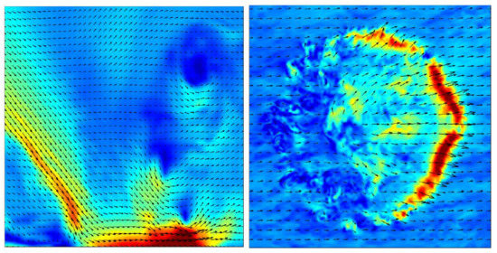
Figure 5 shows the full 3-D wind velocity at km with arrows to denote the projection of the wind speed onto the x-z plane for the cases C1-0x0y, N-0x0y and S2-0x0y at 450 s into the downburst simulations. The arrow lengths are scaled with velocity magnitude. The air parcels travel from the cooling source center aloft ( km, km, km) and, in the presented figure, they are clearly seen to generate strong horizontal winds near the surface after they touch down. At about this time, extreme wind speeds occur at km for both the N and S2 cases, where one might then expect to capture peak values in the time series of velocity in x-direction. It is noticed that the downburst develops slower in the C1 case. This is due to interaction with the ambient turbulence as the downbursts penetrate through the boundary layer and expand radially outward. The outflow winds reach the turbine line of km sooner in the N and S2 cases. A ring vortex is clearly seen near the surface for each case. According to Hawbecker et al. [26], the height of the center of the ring vortex is lower in the convective case (~300 m AGL in the C1 case) compared to the N and S2 cases. The results in the present study show that the lower vortex in the C1 case tends to create stronger extreme winds at the turbine’s hub height.
The velocity fields at the turbine hub height shown in Figure 6 describe the downburst field flow structure at a mature stage, 600 s into each downburst simulation, for the C1-0x0y, N-0x0y and S2-0x0y cases. The turbine’s rotor plane located at km is shown by the dashed white line for reference. Each case shows a band of strong winds downwind from the downburst center. As the atmospheric stability increases, this band is seen to become more organized due to a less turbulent ambient environment allowing for prolonged propagation of intense outflow winds. Immediately behind the strongest outflow wind speeds, it can be seen that the C1 case has an area of trailing high winds that are not apparent in the neutral and stable cases. This organization found within the neutral and stable cases is due, again, to the lack of ambient turbulence impeding the downdraft as well as the outflow winds. Although at this time the wind speed maximum has moved downwind of the turbine line at km for each case, residual effects from the downburst outflow can still be seen along this line. The wind field at km is recorded for the entire duration (life) of the simulated downburst and is used in the aeroelastic turbine modeling discussed in the following sections.
3.2. Effect of Atmospheric Stability on Turbine-Scale Wind Fields
In this study, we extract turbine-scale inflow fields from a 2-D vertical slice at km as was described in Figure 5 and Figure 6. Our focus is on downburst wind fields centered around the middle of the domain in the y-direction (i.e., km for the 0x0y case) so that the influences from lateral winds are reduced. We investigate central winds in the simulated downbursts and their effects on the associated aeroelastic response of the 5-MW wind turbine model.
To assess the influence of atmospheric stability on the velocity at hub height, case 0x0y-X1 is considered for each stability case (C1, C2, N, S1, and S2). The U-, V-, and W-components of velocity for the five stability regimes are presented in Figure 7. Here, we first select the cases of 0x0y-X1 to describe the main characteristics found while other data are also discussed later. There are three distinct periods evident in the time series: (1) pre-downburst (Period I, 0–6 min), (2) intra-downburst (Period II, 6–12 min), and (3) post-downburst (Period III, 12–15 min). In Period I, velocity in all directions remains somewhat stationary with only the convective cases showing some variability due to increased turbulence. When the outflow impacts the wind field at km (Period II), the vertical velocity reaches its maximum value first (updraft) and then drops abruptly in the opposite direction down to a minimum (downdraft). This is because the developed ring vortex passes over the turbine line. Meanwhile, the longitudinal and lateral velocity components reach their peak values around the same time that the vertical velocity reverses direction (i.e., at about 450 s). After the extreme winds have dissipated, in Period III, the longitudinal wind speeds are seen to have decreased. The lateral and vertical winds show greater variations after the impact of the downburst outflow winds.
In the longitudinal velocity variation, we also notice that the velocity peaks are actually associated with a primary surge and lasting intense winds that follow. From the time series of the longitudinal velocity component, primary surges are seen to appear at around 450–500 s while the sustained intense winds that follow occur at around 500–650 s, with an evident slower decaying rate. This phenomenon can be explained by the continuing smaller vortices emerging from the cooling source. After the primary vortex ring has spread outward, there are still cool air parcels aloft that form smaller vortices and in turn generate the lasting intense winds. These sustained winds cause the longitudinal velocity to remain high for a short while ultimately decaying later. These characteristic sustained downburst winds were also reported by Anabor et al. [23]. Since we decreased the time span of the cooling intensity to only six minutes, the duration of the lasting winds seen in the time series is much shorter than those reported by Anabor et al. [23] whose cooling function time span was selected to be 14 min. In our turbine load studies that follow, we will see that even this short period of sustained high winds can play an important role in influencing extreme loads.
We next discuss the effect of stability on the simulated wind fields. In Period I, the lateral velocity component is seen to get larger as the stability increases. This is attributed to the Coriolis forcing, which leads to a direction change in the ambient wind. When the maximum outflow passes over the turbine line, in Period II, the extreme longitudinal velocity component is clearly higher in the convective cases; this is because the ring vortex develops faster in the convective regime and has not yet matured fully in the stable regime at the turbine line by this time. Stronger updrafts driven by the ring vortices in the convective cases are also seen in the higher vertical winds. After the primary surge from the outflow, it is found that the convective cases tend to have stronger winds that follow. There are two reasons for this. First, the ambient wind in the convective cases is almost entirely westerly (see Figure 6), and as a result, when we consider central winds within the downburst, the outflow and ambient winds are in the same direction. The two aligned wind effects (ambient and outflow) increase the net effect in the convective cases. The effect of the ambient wind direction can be also seen in the lateral wind time series, where during the primary surge of the outflow does not change much in the convective cases compared to the significant changes seen in the stable cases. Second, as seen in Figure 5, the ambient turbulence within the C1 case impedes the downdraft as it descends towards the surface. This effectively delays the downburst from reaching the surface and prolongs the strong outflow winds. After the occurrence of the maximum outflow winds, the stable cases are found to be accompanied by greater fluctuations in the lateral and vertical winds during both Periods II and III.
To generalize the characteristics of the turbine-scale wind fields, we examine statistics of selected wind-related parameters extracted from all the 120 generated flow fields, as seen in Figure 8. It is clearly seen that, in Period I, the lateral velocity at hub height () is larger for the stable cases due to the Coriolis effect. Since the longitudinal wind velocity () in this period remains roughly constant at around 6 m/s, the wind direction at hub height (WndDir) deviates by up to about 20° in the stable regime (S2). In Period II, the extreme longitudinal wind velocity, , is noticeably larger in the convective cases because of the quicker development of ring vortex, driving stronger outflows near the surface, as was seen in Figure 5. The effect of the ring vortex is also evident in the statistics; stronger updrafts (max) and downdrafts (min) are noted in the convective cases. Ramp rates of the primary surge in the longitudinal velocity are found to be slightly larger in the stable cases. This can be attributed to reduced interaction between the downdrafts and the ambient wind, with diminished turbulence, as stability increases. These wind field surge ramp rates in Period II are computed at a time when the hub-height wind speed begins to exceed the turbine’s rated wind speed of 11.4 m/s. We will later discuss the significance of these ramp rates on wind turbine extreme loads. The longitudinal velocity after the maximum outflow is seen to be somewhat larger in the C1 and C2 cases compared to the neutral and stable cases. This is attributed to the stronger sustained winds in the convective cases, that were discussed earlier while studying Figure 7. The range from minimum to maximum values of in Period III are also found to be greater for the stable cases; this also results in larger wind direction changes and can lead to higher yawing moment loads on the wind turbine.
3.3. Effect of Location of Cooling Source and ET Ambient Turbulence
Here, we investigate the sensitivity of the outflow winds produced at km to the four locations of the cooling source as mentioned in Section 2 (see Figure 2). In Figure 9, the time series for three velocity components at hub height for the selected cases C1-X1 (left column) and S2-X1 (right column) for all four cooling source locations are presented. The results reveal that the localized turbulence in the different stability regimes for the different cooling source locations can lead to different velocity fields in the downburst outflows, especially in the convective regime. For the C1-X1 case, both the peak value of the outflow gusts as well as the occurrence times of these extreme winds exhibit greater variability due to the stronger turbulence intensity in the ET ambient wind fields, as is especially evident in the longitudinal velocity component’s time series. Fluctuations in the lateral and vertical wind velocity are also more variable. The general characteristics of the outflow surge are more similar for all C1 initial locations (in the time series), except for the 0x5y case which shows a secondary surge almost as high as the primary one. The pattern of an updraft followed by a downdraft is evident in the time series. In the stable case with the different cooling source locations, the maximum outflow during the simulated downbursts are very similar; not much variability in either the peak winds nor in the occurrence time of the same are noted. Fluctuations in the velocities after the maximum outflow are seen to be slightly different due to the variation in the localized turbulence when the cooling source location is changed.
Next, we fix the initial location of the downburst cooling source (at 0x0y) and study differences in the resulting wind fields at six different turbine locations, X1–X6, on a vertical plane where km. The wind velocity for each of the 6 inflow fields in the selected stability cases, C1 and S2, are presented in Figure 10. The inflow field X1 is selected at the center (laterally) of the simulation domain (i.e., at km). All the other partially overlapping inflow fields are also selected on the plane, km, and extend northward up to X6 (see Figure 3). Since the Coriolis force causes a turning of the ambient wind towards the north as the stability increases, as seen in the curves for the S2 case, sustained winds after the outflow are seen to be larger as the turbine location is moved from X1 to X6. This same trend is not evident in the C1 case because the ambient wind direction does not change very much in the convective stability regime. In the lateral wind time series for the S2 case, differences in the ambient wind direction, among the X1–X6 cases, can be also seen; the maximum outflow has the lowest peak value of (negative peak) for X6. This is because in the stable case the downburst touchdown center is pushed further north due to the turning of ambient winds; therefore, the downburst winds cause the negative V-component velocity when we look at the center of the domain. The wind field at the northern most location, X6, is the closest in alignment with the mean ambient winds and has the most positive value of the peak. In general, the velocities in the six cases, X1–X6, are seen to have very similar peak values and peak occurrence times for the convective cases. As such, it is only in the stable case, that differences in ambient wind direction and in lateral winds arise and these affect the sustained winds only after the primary surge.
4. Assessment of Wind Turbine Loads
To assess turbine loads during simulated downburst winds, we consider three response variables—the out-of-plane blade root bending moment (OoPBM), the tower base fore-aft bending moment (FATBM), and the tower-top yawing moment (TTYM). These variables are often of interest when studying turbine performance in different external conditions. We first investigate the relationship between turbine loads, the inflow wind velocity field, and the turbine control systems. Later, the influence of contrasting atmospheric stability is discussed.
4.1. Effect of Wind Velocity Field and Turbine Control System
Figure 11 shows time series of the horizontal and vertical wind speed at hub height, the blade pitch angle, the hub-height wind direction, the nacelle yaw angle, the yaw error (misalignment between wind direction and yaw angle), and the three turbine load variables—OoPBM, FATBM and TTYM—over the entire downburst simulation for the selected case, N-0x0y-X1. As can be seen, the blade pitch angle variation with time (in red) indicates a discrete triangle-shaped variation over the period when the horizontal wind speed exceeds the rated wind speed (11.4 m/s). When the blade pitch angle is increased, there is direct reduction in the impact on loads from the streamwise winds and a resulting double-peak time series for both OoPBM and FATBM. The interval between the two peaks is determined by the sharpness of the pitch angle triangle. In the presented case, N-0x0y-X1, the extreme bending moment at both the blade root and the tower base are indicated at the first peak and denoted by red diamond marks. The first 300 s of the load time series are basically related to spin-up (transient vibrations) of the FAST model. This transient response, obvious at the beginning of FATBM time series, for example, is not taken into account when computing fatigue and extreme loads. In contrast, the tower-top yawing moment is related more to the wind direction change and related yaw error. A certain amount of wind direction change is evident at the beginning of Period I because of the Coriolis force; however, the yaw control system can keep up with this initial wind direction change and can limit the yaw error. This mechanism allows the TTYM load to remain close to zero during Period I. With the occurrence of peak outflow winds, the nacelle yaw angle is no longer well-controlled due to an excessively rapid wind direction change (and a maximum permissible nacelle yaw rate set at 0.3°/s); as a result, the yaw error starts to show larger fluctuations in Period II. These fluctuations result in large variability in TTYM loads after the maximum outflow. Since the yaw moments result from unbalanced and asymmetric loading on the three blades, both the streamwise wind surge and the wind direction changes can influence TTYM load levels. Of these two influences, the streamwise wind surge, because of the mitigating effect of pitch control, has a smaller effect on the yaw moment compared to its effect on OoPBM and FATBM. In addition, at around 400 s, there is a clear up-and-down rapidly fluctuating pattern in the TTYM time series, which is related to the updraft and the immediately following sudden downdraft seen in the variation. Thus, the vertical wind velocity component is also found to influence the tower-top yaw moment, although its influence on blade root and tower base bending moments is insignificant.
In general, patterns in the OoPBM and FATBM time series are closely related to the time series of the hub-height horizontal velocity and the blade pitch angle. The TTYM time series, on the other hand, are seen to be related to both the horizontal and vertical velocities as well as to yaw error, resulting from rapid wind direction changes. Additionally, larger variations in the TTYM load result from asymmetric loading on the three blades.
4.2. Effect of Atmospheric Stability
Figure 12 shows time series of the three turbine loads—OoPBM, FATBM, TTYM—in the selected case, 0x0y-X1, for the five different atmospheric stability conditions. In the OoPBM and FATBM time series, pitch control actions cause load reductions around 400–600 s and the double-peak variation with time is evident. The interval of time between the two peaks is longer for the convective cases. This can again be explained by the longer lasting sustained winds, in the convective cases, after the primary surge of the downburst (as we saw in Figure 7). The second load peak appears both delayed and somewhat higher in the convective cases; these second peaks imply larger extreme loads than the earlier stronger winds in Period II and greater risks to the turbine structure. On the other hand, the TTYM loads are more sensitive to vertical winds and yaw error resulting from rapid horizontal wind direction change. It is found that the rapidly fluctuating up-and-down patterns seen in the yaw moment time series are more intense in magnitude in the convective cases and could lead to higher extreme loads (than for neutral and stable conditions). These larger TTYM loads are related to the larger updrafts in the convective cases that we saw earlier in the vertical velocity time series. In other words, for a downburst that initiates in a convective boundary layer, yaw moments tend to reach higher levels as the ring vortex passes over the turbine. Since there is greater variability in lateral and vertical velocities for the stable cases after the extreme outflow winds (see Figure 7), the TTYM time series also show greater fluctuations with increasing stability and this, in turn, leads to extreme loads after the maximum outflows. Studying the yaw moment time series, we find that extreme loads in the convective cases tend to be influenced by the ring vortices, while extremes in the stable cases occur later and are corresponding to the sustained and largely fluctuating loads.
We turn next to a study of the influence of atmospheric stability on fatigue loads on the wind turbine. Figure 13 shows the histograms of turbine load ranges, computed using the rainflow cycle-counting algorithm. As seen in the nine histograms presented, that largest number of cycles have amplitudes that are very small (close to zero). For all three loads, a greater number of high-amplitude cycles occur for the convective cases than for the stable cases, even though the actual high-amplitude bin counts are very small. Generally speaking, higher winds causing higher amplitude load cycles; this is consistent with our earlier finding that the maximum longitudinal wind speed is larger for the convective case, as we saw in Figure 8. With increasing stability, the total number of cycles of the OoPBM and TTYM time series increases but with the greatest increase seen for the lowest amplitude cycles; a clear trend is not evident for FATBM loads. These results suggest that fatigue damage associated with the OoPBM and TTYM loads is reduced as atmospheric stability increases; more low-amplitude cycles but fewer high-amplitude cycles influence the EFL calculated according to Equation (6). The difference in EFL values for the various stability cases will be discussed via statistical analyses.
4.3. Effect of Cooling Source Location and Turbine Position
We consider now the influence of the initial location of the downburst cooling source on turbine loads. Figure 14 shows time series of the three turbine loads for the selected cases, C1-X1 and S2-X1, with four different locations of the cooling source. Based on the wind velocities that were presented in Figure 9, the load time series show considerable variability in the C1 case, for which velocity time series also showed significant variability when the different cooling source locations are considered. Although the double-peak characteristics are evident in both the OoPBM and FATBM time series, the two peaks are different in both extreme values and in their occurrence times as a result of the greater ambient turbulence in the convective regime. In contrast, the load time series in the S2 case are seen to be not very different from each other, with only slight fluctuations after the maximum outflow, for the four different cooling source locations. This can be attributed to the turbulent sustained winds after the primary surge, even in the stable case. The time series for the yaw moment reveal no consistent characteristics among the four C1 cases. In the stable case, the yaw moment is influenced by the turbulence of the sustained winds after the extreme outflow and thus reveals different extreme values for the four cooling source locations.
Figure 15 compares time series of turbine loads for six different turbine locations for the selected cases, C1-0x0y and S2-0x0y. As mentioned in Section 3.3, the main difference in the inflow fields, X1–X6, is the deviation of the outflow wind from the ambient wind and stronger sustained winds after the primary outflow surge in the stable regime. The OoPBM and FATBM turbine loads are all very similar in the C1 case and the time series exhibit similar first peaks, even for the S2 case. The second peaks for the stable case occur later and with larger peak widths (i.e., the peaks are sustained over a longer time) for the X6 inflow field since the stronger and more sustained winds keep the load high after earlier pitch control actions. The yaw moments, sensitive to asymmetric loading, are influenced more by turbulence and are, thus, exhibit greater variability with changes in turbine locations for both the C1 and S2 cases.
4.4. Scenarios of Extreme Loads
Since extreme loads are indicators of potential risks to turbine structures, we study next the pattern of occurrence of extreme loads during downbursts. Based on the conclusions in Section 4.1, the time series of the horizontal wind speed at hub height and the blade pitch angle are important to consider. Accordingly, we examine all the peak values in time series of turbine loads and study them in conjunction with time series of the horizontal wind speed and associated blade pitch angle. Figure 16 shows four typical scenarios seen in the OoPBM time series and selected from all the 120 FAST runs. Scenarios 1 and 2 show load peaks that appear at the start and end times of a triggered pitch control action interval (red curves). The load peaks in Scenarios 3 and 4 appear, respectively, during the pitch control action interval and a short while after. Among the four scenarios, only the extreme loads in Scenario 1 result from the primary surge of the downburst. The other scenarios are caused by sustained intense winds that occur after the extreme outflow. In Scenario 2, the sustained winds are high enough to trigger pitch control action and bring about a ”big triangle” appearance to the pitch angle time series; the extreme load then occurs at the end of this triangle. In Scenario 3, there is an obvious secondary surge in the sustained winds after the initial peak outflow. The extreme load occurs between the primary surge and the secondary surge in the brief period when blade pitch control actions are inactive. In our study, consecutive surges in a downburst are rare and are only found in the case, C1-0x5y, where turbulent updrafts play a significant role in modifying the downburst structure. Finally, in Scenario 4, the sustained winds, after the peak outflow are too low to activate the blade pitch control and thus extreme loads result, even with relatively low wind speeds.
Figure 17 compares extreme load occurrence scenarios for the atmospheric stability cases of C1, N and S2. Wind fields for 5x5y-X6 are selected for illustration. For the FATBM loads, fluctuations in the time series are seen to be very similar to that for OoPBM. However, extreme loads can occur in different scenarios. As seen in the figure, FATBM loads are very sensitive to the primary outflow surge so that, in all three atmospheric stability cases, the extreme loads appear according to Scenario 1. The OoPBM loads also exhibit peak values related to the primary surge of the outflow but, in this example, extreme loads occur at or after the end time of the big triangle. As the stability increases, the ramp rate of the primary outflow surge gets larger (as seen in Figure 8). This, therefore, results in an increase in the extreme levels of the FATBM loads. As may be expected, the largest tower base bending moment (FATBM) results from the maximum downburst winds. The sustained winds after the maximum outflow only cause minor effects. On the other hand, the TTYM loads are associated with unbalanced loading on the turbine rotor and lead to more variability in the scenario that describes extreme loads. The extreme load is sometimes seen to be related to the primary surge of outflows (i.e., case N); however, this load is also sensitive to vertical winds and yaw error. Together, all these effects lead to greater uncertainty in the TTYM extreme load scenarios. In an earlier study, we have found that pitch control actions have a smaller influence on TTYM loads than on OoPBM and FATBM [35]. In summary, the extreme yaw moment may not occur at a time that corresponds exactly to the start or end time of the triggered pitch control interval, as can be seen in Figure 17.
We briefly compare our findings to those in Nguyen et al. [9], a previous downburst study using a stochastic-analytical hybrid model. With the non-turbulent portion of the downburst winds modeled by analytical functions, the time series of turbine blade root bending moment also showed a double-peak pattern, but the extreme load was found to rarely occur according to Scenario 1. This is attributed to the fact that the analytical model underestimated the rapid increase in the primary outflow surge which is found to be significant in the present study based on use of an LES model. In another study of downburst winds and associated turbine loads, Nguyen et al. [10] reported that effective yaw control can have a significant influence on the tower-top yaw moment. That work considered downburst scenarios that resulted in larger yaw errors (sometimes even greater than 45°) and more extreme wind speeds than in the present study; as such, the maximum yaw moment values in our study are not comparable to those in the cited study (where TTYM maxima were about 27 MN-m).
4.5. Wind Velocities and Extreme Loads
In this section, we further study the turbine-scale wind structures during a downburst and its relationship to the occurrence of extreme loads. Figure 18a compares the variation with time of hub-height wind fields of selected turbine-scale slices for the C1, N and S2 cases. The changing resultant wind direction is also denoted by arrows. The occurrence times of extreme values of OoPBM, FATBM and TTYM are denoted by red markers with the letters O, F and T, respectively, written on the time axes. In Period I (0–360 s), we see the effect of the Coriolis force turning the wind direction towards the northeast (towards the upper-right in Figure 6) as the stability is increased. When the maximum outflow occurs, the wind direction does not change much in the C1 case but it turns more clearly to the lower-right (southeast) with increasing stability. This is due to the center of the downburst being displaced to the north-east as described in the previous section. After the maximum outflow, there are more fluctuations in wind speed for the C1 case but more fluctuations in wind direction for the S2 case. Due to interaction with the ambient winds mentioned before, it is also seen that, in the C1 case, the sustained winds are stronger while the wind speed peak is delayed by about 20–30 s. It is found that extreme FATBM loads generally tend to occur at a time right before the maximum outflow (Scenario 1). Thus, the higher ramp rates for wind speed in the stable cases could lead to larger extreme loads than in the convective cases. On the other hand, TTYM loads are related more clearly to wind direction changes. Therefore, the large fluctuations in wind direction in the stable cases could cause more frequent occurrences of large TTYM loads after the maximum outflow. Extreme OoPBM loads can be related to both the primary surge and the sustained intense winds of the downburst. The ramp rate of the primary outflow surge can also affect OoPBM extreme loads in Scenario 1.
Figure 18b shows similar filled contours representing the time-varying wind fields on a vertical line at the center of the turbine rotor plane. In Period I, the vertical wind velocity appears stationary and close to zero for all the stability cases. After the downbursts touch down, the developed ring vortices passing over the turbine line (Figure 5) bring updrafts first and then downdrafts. Extreme wind speeds appear when the vertical wind components are close to zero. The vertical wind shear generated by the ring vortex is clearly seen in each case. Hawbecker et al. [26] noted that there might be more complex patterns of vertical wind shear due to downbursts for the N and S2 cases. Since we are considering only turbine-scale wind fields, the wind speed in all cases is seen to simply decrease from the surface to the top of the rotor plane. The center of the ring vortex, closer to the surface in the C1 case, also leads to larger extreme wind speeds as seen in the contours. Please note that larger extreme winds do not necessarily result in larger extreme loads since pitch control actions can mitigate the impact of strong winds. For OoPBM and FATBM (and especially for FATBM), large ramp rates of the primary surges more directly influence extreme loads. Hawbecker et al. [26] noted that the N and S2 cases exhibit stronger vertical velocities associated with the ring vortex, on average, than the C1 cases. Here, we see one case in which the vertical velocities associated with the ring vortex are slightly larger for the convective case. The influence of vertical winds on turbine loads is considered to be rather small for the OoPBM and FATBM loads, whereas their effect found on TTYM loads can be significant.
We are also interested in examining the wind structure over the rotor plane when the extreme loads occur. Figure 19 shows filled contours of velocity of the inflow fields extracted at the time of occurrence of extreme loads for three cases—C1, N, and S2—for the 0x0y-X1 case. Snapshots at s (i.e., indicating the initial fields with the different stabilities) are also shown for comparison. These figures correspond to viewing of the wind field looking upwind or to the west (i.e., towards the downburst center). As seen in the figure, the initial ambient wind fields indicate weaker winds compared to the more intense downburst winds to follow; the C1 case presents a bit more turbulence than the other two cases, the S2 case in contrast shows more organized shear. Coriolis forcing is evident initially with all the V-component winds directed to the right (+y-direction). The extreme loads generally appear to occur at a time prior to the maximum outflow when the pitch control action is triggered (Scenario 1). Thus, one can see that, for example, in all cases, the wind fields at the time of extreme FATBM are relatively weak (wind speeds around 10 m/s) and are accompanied by updrafts (upward pointing arrows). In the C1 case, the extreme TTYM occurs slightly later than the other two load extremes for that case—the turbine experiences strong outflow winds with a non-uniform pattern (weaker on the left) which causes unbalanced rotor loading and large yaw moments. In the S2 case, the extreme OoPBM occurs after the maximum outflow has occurred and when the pitch control action is not in place anymore (Scenario 2), while the TTYM load, not dependent on pitch control, reaches its peak a short while later (Scenario 4). In these last scenarios, the turbine experiences strong outflow winds at the tower base (as seen in Figure 18b) together with downdrafts. The lateral winds also reach their maximum magnitudes in the negative y-direction (left-down arrows). Rapid changes in the horizontal direction might, again, lead to asymmetric loading as well as extreme yaw moments.
4.6. Statistical Analysis of Fatigue and Extreme Loads
With a view towards generalizing some results from this study, we select six turbine locations around the center line of the downburst trajectory (i.e., X1–X6) together with four locations of the downburst cooling source (i.e., 0x0y, 5x0y, 0x5y and 5x5y) and report on statistics of turbine loads. Emphasis is primarily on the influence of atmospheric stability on fatigue loads (EFL) and extreme loads (ExL). Due to the different materials used in the structural components of the wind turbine, the Wöhler exponent in the EFL calculations are set to 10, 6, and 3, respectively, for OoPBM, TTYM, and FATBM. We present box plots of turbine load statistics for the different stability regimes in Figure 20. As seen in the plots for fatigue loads, there is a clear trend which suggests that the OoPBM mean EFL values decrease with increasing stability; an explanation for this is that higher extreme outflows in the convective cases tend to cause more high-amplitude load cycles (Figure 13), which in turn increase the EFL value. This trend is not as clear with FATBM loads, where EFL values even in a stable case can be as high as those in the convective cases. This can be attributed to the generally higher extreme loads in stable cases (compared to convective) for the FATBM loads as seen in the right-panel middle plot, which then directly leads to greater EFL values as well. Extreme FATBM loads mostly occur right when pitch control actions start (i.e., Scenario 1); it is the larger ramp rate of the primary surge in the stable cases that leads to the higher extreme loads as well as elevated fatigue loads. This observation is consistent with the extreme loads indicated in the time series presented in Figure 17. The extreme OoPBM and TTYM loads do not generally occur according to Scenario 1; hence, the noted trend for FATBM is not evident in the box plots for OoPBM and TTYM extremes. The extreme yaw moment, as was discussed in Section 4.2, is influenced more strongly by the impact of the ring vortex in the convective cases, where updrafts and downdrafts are stronger. The extreme TTYM load in the stable cases is mostly a result of the larger yaw errors after the maximum outflows have passed. This is why the mean TTYM ExL is still higher in the convective cases. Similarly, TTYM fatigue loads are also higher for the convective cases, but greater uncertainty seen in the neutral and stable cases obscure a clear decreasing trend with increasing stability.
We briefly compare loads from this study to those reported in earlier studies [10,13] that used an analytical model to simulate non-turbulent downburst winds with superimposed stochastic turbulence. See Table 3. Case 3b from Nguyen et al. [10] represents an idealized case while Case 2 from Nguyen et al. [13] describes an average or representative downburst from the JAWS (Joint Airport Weather Studies) project with IEC Kaimal-based non-stationary turbulence. The case C1-0x0y-X1 from the present study is selected for this comparison as it produced the highest extreme wind speed and relatively large turbine loads compared to the other stability cases and runs. As can be seen from the table, the maximum wind speed for this selected case is much lower than that in Case 3b [10] which in turn produced lower extreme OoPBM and TTYM loads. The maximum wind direction change for Case 3b [10] was also significantly larger; this led to large yaw errors as well as greater extreme yaw moments (more than four times larger than in the present study). We note, however, that the LES model employed in the present study led to faster rates of change in wind speed and wind direction that may also be interpreted as underestimations by the analytical model. The rate of change in the primary outflow surge, especially, is considered to be significant in the extreme load scenarios and resulting load levels. Compared to the Case 2 in Nguyen et al. [13], the present study shows somewhat lower extreme wind speeds; the maximum wind direction change, however, is again not comparable. This is because only centerline winds at one location along the downburst track were considered in this study. The extreme OoPBM load in the present study is slightly lower while the fatigue load is larger. These results suggest that the rapid change in wind speed and direction captured in the LES model may influence fatigue loads that are again underestimated in the analytical model, even with the higher outflow winds.
In a previous study by some of the authors [35], the change in atmospheric stability over the evening transition (ET) period was found to have a significant effect on turbine loads. Downbursts, which often occur in the ET period, could greatly increase turbine loads (relative to ambient ET conditions) to different degrees depending on the atmospheric stability. Accordingly, we evaluate next the ratio of extreme loads during or after the maximum outflow in a downburst (in Periods II and III) to those during the ET period before the maximum outflow (i.e., in Period I). These ratios are computed for all the 20 FAST runs of the X1 turbine location; we compare the ratios for the different stabilities in Figure 21. Four different cooling source locations are considered for each of the five stabilities. For the extreme or peak loads in Period I used in computing the ratio, the first 100 s of each load time series are discarded to eliminate transient effects in the response computed in the FAST simulations. Our focus is on understanding the degree to which extreme loads are enhanced during a downburst as a function of the atmospheric stability conditions. As seen in the figure, after the downburst’s maximum outflow, all the extreme loads are about 2–7 times larger. The extreme OoPBM and FATBM load ratios are, in general, larger as the stability increases. These results suggest that although OoPBM and FATBM loads may be relatively low in a stable boundary layer [35], they could reach relatively high levels after a downburst. The trend in extreme TTYM increase is less clear. Since the yaw moment is greatly influenced by turbulence, the ExL increase ratio in the convective case shows both the greatest variability and attains the largest values.
In Hawbecker et al. [26], a conclusion was drawn that stronger winds in simulated full-domain fields persist for a longer duration under stable conditions. In our own investigations of the turbine-scale flow field at the centerline location, it is found that the ring vortices in stable regimes pass through the turbine line km quicker and tend to cause intense primary surges of outflow winds; these, in turn, lead to larger FATBM extreme loads (Figure 20). The increase in OoPBM and FATBM extreme loads during a downburst is also significant in the stable case. However, because of the lower extreme horizontal winds at this location, weaker sustained winds after the maximum outflow, and smaller updrafts and downbursts in the stable regimes, OoPBM and TTYM fatigue and extreme loads are still seen to be somewhat larger when downbursts touch down in the convective boundary layer.
5. Conclusions
In this study, we modeled idealized downbursts initiated during various stability regimes by means of a pseudo-spectral LES model together with a cooling source mimicking the evaporative cooling of the downburst. Full-domain slices of 2-D wind fields were extracted from the LES-generated fields for each downburst at a distance 3.5 km downwind of the cooling source center. Then, several turbine-scale wind fields were extracted from the lowest portion of the 2-D slices to serve as inflow fields that were input into a NREL 5-MW turbine model for the assessment of downburst-associated turbine loads. Using these simulated flow fields, characteristics of turbine-scale downburst flow fields under different environmental stabilities were discussed. Relationships among the velocity time series, turbine control actions and turbine loads were studied. A statistical analysis was performed using simulated flow fields around the center line of the downburst trajectory in order to investigate fatigue and extreme loads on the selected wind turbine.
Upon studying the downburst wind velocity fields at turbine scale (with a focus on the centerline along the downburst track), we found that, for the convective cases, the extreme horizontal winds are higher and the sustained winds after the maximum outflow are larger compared to the neutral and stable cases. In contrast, fluctuations in the lateral wind velocity increase as the atmospheric stability increases. An earlier study by Hawbecker et al. [26], for the full-domain fields, found that stronger winds persisted for longer durations under stable atmospheric conditions; nevertheless, when focusing on the central wind field close to the touchdown center (i.e., 3.5 km), estimated fatigue loads on wind turbines still generally decrease as stability increases since turbine loads are most influenced by the primary outflow surge and the sustained intense winds that follow. Upon studying load time series, we found that OoPBM and FATBM loads are greatly influenced by the horizontal wind and by pitch control, whereas TTYM loads are influenced by the impact of the ring vortices (and associated rapid direction change in vertical winds) and by increased yaw errors after the maximum outflow. The interplay of changing velocity in a downburst and blade pitch control also results in four scenarios that can explain the occurrence of extreme loads. Lastly, results of a statistical analysis revealed that extreme loads, different from fatigue loads, do not systematically decrease with increasing stability. This can be further explained by the different characteristics of the extreme load scenarios corresponding to the three types of turbine loads. Comparing extreme loads before and after the maximum outflow, we found that increases in extreme loads in a downburst over pre-downburst values were larger for those downbursts that initiated in stable boundary layers.
Compared to the earlier studies of downbursts modeled using a stochastic-analytical hybrid model [9,10,13], we found that the LES model can capture the main characteristics of downbursts and uncover similar patterns in turbine load time series. The LES model is seen to result in velocity fields with more rapid changes in wind speed and direction, which are not seen with the analytical model. These rapid changes are found to have an important influence on associated extreme and fatigue loads.
We found that the current IEC load cases model extreme gusts with highly simplified analytical functions that are inadequate, based on results from the present study. A possible way to refine the current gust functions, for transient events such as downbursts, is to consider physical details captured from the LES runs in this study and modify load case gust parameters to achieve more realistic loads. The initial ambient stability prior to the downburst event should also be taken into account as it can be a key factor in defining a new gust model for inflow generation in turbine design for some limit states.
Future efforts on similar work to that described here could focus on downbursts covering an area that is spread farther out beyond the center line. It is expected then that greater wind direction changes would result during the downburst winds and highlight the significance of yaw control in the turbine model. The studies can also be further extended to help undertake a risk assessment of a wind farm struck by a downburst with various initial stability regimes.
The LES model in our study still falls short of considering realistic environmental parameters that could cause different stability regimes in which downbursts could be initiated. Future works could examine different microphysics parameterizations with the LES model and then seek to generate downburst winds under realistic conditions. For instance, based on our investigations, the time span of the downburst cooling source function is a parameter that is expected to have a great impact on the intensity of sustained vortices and high winds after the primary surge and, in turn, on the turbine loads. Understanding how this parameter relates to realistic atmospheric conditions and studying its effect systematically would be of value in estimating the risks of wind turbine structures struck by downburst winds.
Author Contributions
N.-Y.L. prepared a draft of this manuscript and performed all the wind turbine loads simulations as part of his doctoral studies; he also analyzed the large-eddy simulations (LES) that were generated by P.H. and generated wind turbine inflow velocity fields from the LES model output. S.B. supervised efforts of the second author and the LES model was developed based on his in-house code. The second and third authors prepared a plan for the downburst simulations and developed the LES velocity field database. L.M. supervised the work of the first author and the two together conceived of the wind turbine loads studies; the fourth author served as the dissertation advisor of the first author and helped with the first draft of the paper and was ultimately responsible for the editing and final preparation of the manuscript.
Funding
This research was funded by the National Science Foundation (NSF) under Grant Nos. 1336304 and 1336760.
Acknowledgments
The authors gratefully acknowledge the Texas Advanced Computing Center (TACC) at The University of Texas at Austin for providing HPC resources that have contributed to the research results reported within this paper. All the LES computational studies in this paper were carried out on the Stampede system at TACC [43]. URL: http://www.tacc.utexas.edu.
Conflicts of Interest
The authors declare no conflict of interest.
References
- Fujita, T. The Downburst; SMRP Research Paper Number 210; Department of the Geophysical Sciences, The University of Chicago: Chicago, IL, USA, 1985. [Google Scholar]
- Fujita, T. Downbursts: Meteorological features and wind field characteristics. J. Wind Eng. Ind. Aerodyn. 1990, 36, 75–86. [Google Scholar] [CrossRef]
- Fujita, T.; Byers, H. Spearhead echo and downburst in the crash of an airliner. Mon. Weather Rev. 1977, 105, 129–146. [Google Scholar] [CrossRef]
- Fujita, T. DFW Microburst; SMRP Research Paper Number 217; Department of the Geophysical Sciences, The University of Chicago: Chicago, IL, USA, 1986. [Google Scholar]
- Hawbecker, P.; Basu, S.; Manuel, L. Realistic simulations of the July 1, 2011 severe wind event over the Buffalo Ridge Wind Farm. Wind Energy 2017, 20, 1803–1822. [Google Scholar] [CrossRef]
- International Electrotechnical Commission. Wind Turbines-Part 1: Design Requirements; Technical Report, IEC-61400-1; IEC: Geneva, Switzerland, 2007. [Google Scholar]
- Orwig, K.; Schroeder, J. Near-surface wind characteristics of extreme thunderstorm outflows. J. Wind Eng. Ind. Aerodyn. 2007, 95, 565–584. [Google Scholar] [CrossRef]
- Nguyen, H.; Manuel, L.; Veers, P. Wind turbine loads during simulated thunderstorm microbursts. J. Renew. Sustain. Energy 2011, 3, 053104. [Google Scholar] [CrossRef]
- Nguyen, H.; Manuel, L. Thunderstorm downburst risks to wind farms. J. Renew. Sustain. Energy 2013, 5, 013120. [Google Scholar] [CrossRef]
- Nguyen, H.; Manuel, L.; Jonkman, J.; Veers, P. Simulation of thunderstorm downbursts and associated wind turbine loads. J. Sol. Energy Eng. 2013, 135, 021014. [Google Scholar] [CrossRef]
- Nguyen, H.; Manuel, L. Transient Thunderstorm Downbursts and Their Effects on Wind Turbines. Energies 2014, 7, 6527–6548. [Google Scholar] [CrossRef] [Green Version]
- Nguyen, H.; Manuel, L. A Monte Carlo simulation study of wind turbine loads in thunderstorm downbursts. Wind Energy 2015, 18, 925–940. [Google Scholar] [CrossRef]
- Nguyen, H.; Manuel, L. Extreme and fatigue loads on wind turbines during thunderstorm downbursts: The influence of alternative turbulence models. J. Renew. Sustain. Energy 2015, 7, 013102. [Google Scholar] [CrossRef]
- Oseguera, R.; Bowles, R. A Simple, Analytical 3-D Downburst Model based on Boundary Layer Stagnation Flow; Technical Report, NASA Technical Memorandum 100632; NASA: Hampton, VA, USA, 1988.
- Chay, M.; Albermani, F.; Wilson, R. Numerical and analytical simulation of downburst wind loads. Eng. Struct. 2006, 28, 240–254. [Google Scholar] [CrossRef] [Green Version]
- Bowles, R.; Frost, W. (Eds.) Wind Shear/Turbulence Inputs to Flight Simulation and Systems Certification; NASA-CP-2474; NASA: Hampton, VA, USA, 1987.
- Vicroy, D. A Simple, Analytical, Axisymmetric Microburst Model for Downdraft Estimation; Technical Report, NASA Report TM 104053; NASA: Hampton, VA, USA, 1991.
- Smith, M. Visual observations of Kansas downbursts and their relation to aviation weather observations. Mon. Weather Rev. 1986, 114, 1612–1616. [Google Scholar] [CrossRef]
- Kessinger, C.; Parsons, D.; Wilson, J. Observations of a storm containing misocyclones, downbursts, and horizontal vortex circulations. Mon. Weather Rev. 1988, 116, 1959–1982. [Google Scholar] [CrossRef]
- Wakimoto, R. Convectively driven high wind events. In Severe Convective Storms; Springer: Berlin, Germany, 2001; pp. 255–298. [Google Scholar]
- Lundgren, T.; Yao, J.; Mansour, N. Microburst modelling and scaling. J. Fluid Mech. 1992, 239, 461–488. [Google Scholar] [CrossRef]
- Hawbecker, P. The Influence of Ambient Stability on Downburst Winds. Ph.D. Thesis, North Carolina State University, Raleigh, NC, USA, 2017. [Google Scholar]
- Anabor, V.; Rizza, U.; Nascimento, E.; Degrazia, G. Large-eddy simulation of a microburst. Atmos. Chem. Phys. 2011, 11, 9323–9331. [Google Scholar] [CrossRef]
- Vermeire, B.; Orf, L.; Savory, E. Improved modelling of downburst outflows for wind engineering applications using a cooling source approach. J. Wind Eng. Ind. Aerodyn. 2011, 99, 801–814. [Google Scholar] [CrossRef]
- Aboshosha, H.; Bitsuamlak, G.; El Damatty, A. Turbulence characterization of downbursts using LES. J. Wind Eng. Ind. Aerodyn. 2015, 136, 44–61. [Google Scholar] [CrossRef]
- Hawbecker, P.; Basu, S.; Manuel, L. Investigating the impact of atmospheric stability on thunderstorm outflow winds and turbulence. Wind Energy Sci. 2018, 3, 203. [Google Scholar] [CrossRef]
- Haines, M.; Taylor, I. Numerical investigation of the flow field around low rise buildings due to a downburst event using large eddy simulation. J. Wind Eng. Ind. Aerodyn. 2018, 172, 12–30. [Google Scholar] [CrossRef] [Green Version]
- Orf, L.; Kantor, E.; Savory, E. Simulation of a downburst-producing thunderstorm using a very high-resolution three-dimensional cloud model. J. Wind Eng. Ind. Aerodyn. 2012, 104, 547–557. [Google Scholar] [CrossRef]
- Orf, L.; Oreskovic, C.; Savory, E.; Kantor, E. Circumferential analysis of a simulated three-dimensional downburst-producing thunderstorm outflow. J. Wind Eng. Ind. Aerodyn. 2014, 135, 182–190. [Google Scholar] [CrossRef]
- Bryan, G.H.; Wyngaard, J.C.; Fritsch, J.M. Resolution requirements for the simulation of deep moist convection. Mon. Weather Rev. 2003, 131, 2394–2416. [Google Scholar] [CrossRef]
- Sim, C.; Basu, S.; Manuel, L. On Space-Time Resolution of Inflow Representations for Wind Turbine Loads Analysis. Energies 2012, 5, 2071–2092. [Google Scholar] [CrossRef]
- Anderson, J.; Orf, L.; Straka, J. A 3-D model system for simulating thunderstorm microburst outflows. Meteorol. Atmos. Phys. 1992, 49, 125–131. [Google Scholar] [CrossRef]
- Li, C.; Li, Q.; Xiao, Y.; Ou, J. A revised empirical model and CFD simulations for 3D axisymmetric steady-state flows of downbursts and impinging jets. J. Wind Eng. Ind. Aerodyn. 2012, 102, 48–60. [Google Scholar] [CrossRef]
- Park, J.; Basu, S.; Manuel, L. Large-eddy simulation of stable boundary layer turbulence and estimation of associated wind turbine loads. Wind Energy 2014, 17, 359–384. [Google Scholar] [CrossRef]
- Lu, N.-Y.; Basu, S.; Manuel, L. On Wind Turbine Loads during the Evening Transition Period. Wind Energy 2019. [Google Scholar] [CrossRef]
- Basu, S.; Portė-Agel, F. Large-eddy simulation of stably stratified atmospheric boundary layer turbulence: A scale-dependent dynamic modeling approach. J. Atmos. Sci. 2006, 63, 2074–2091. [Google Scholar] [CrossRef]
- Orf, L.; Anderson, J.; Straka, J. A three-dimensional numerical analysis of colliding microburst outflow dynamics. J. Atmos. Sci. 1996, 53, 2490–2511. [Google Scholar] [CrossRef]
- Jonkman, J.; Butterfield, S.; Musial, W.; Scott, G. Definition of a 5MW Reference Wind Turbine for a Offshore System Development; Technical Report NREL/TP-500-38060; National Renewable Energy Laboratory: Golden, CO, USA, 2007.
- Jonkman, J.; Buhl, M. FAST User’s Guide; Technical Report NREL/EL-500-38230; National Renewable Energy Laboratory: Golden, CO, USA, 2005.
- Jonkman, B.; Jonkman, J. ReadMe File For FAST v8. 08.00 c-bjj; National Renewable Energy Laboratory: Golden, CO, USA, 2014.
- Sutherland, H. On the Fatigue Analysis of Wind Turbines; Technical Report SAND99-0089; Sandia National Laboratories: Albuquerque, NM, USA, 1999.
- American Society for Testing and Materials. Standard Practices for Cycle Counting in Fatigue Analysis; Technical Report E1049-85; American Society for Testing and Materials: West Conshohocken, PA, USA, 2011. [Google Scholar]
- Prabhat; Koziol, Q. Texas Advanced Computing Center. In High Performance Parallel I/O; Chapman and Hall/CRC: Boca Raton, FL, USA, 2014; Chapter 7. [Google Scholar]
Figure 1.
Three phases in the procedure for generating downburst wind fields during period of contrasting atmospheric stability.
Figure 1.
Three phases in the procedure for generating downburst wind fields during period of contrasting atmospheric stability.

Figure 2.
Schematic diagrams showing four different cooling source locations, with associated downburst simulation domain (dark 10 km × 10 km square), immersed within simulated ET fields shown with lighted lines and labeled 1, 2, 3 and 4, respectively. The labeled fields are repeated based on the periodic padding at the boundaries.

Figure 3.
Schematic diagram showing the overall procedure for the inflow generation and wind turbine response simulation during a thunderstorm downburst.
Figure 3.
Schematic diagram showing the overall procedure for the inflow generation and wind turbine response simulation during a thunderstorm downburst.

Figure 4.
Control characteristics showing variation of blade pitch angle, rotor speed and output power as a function of the inflow wind speed at hub height.
Figure 4.
Control characteristics showing variation of blade pitch angle, rotor speed and output power as a function of the inflow wind speed at hub height.
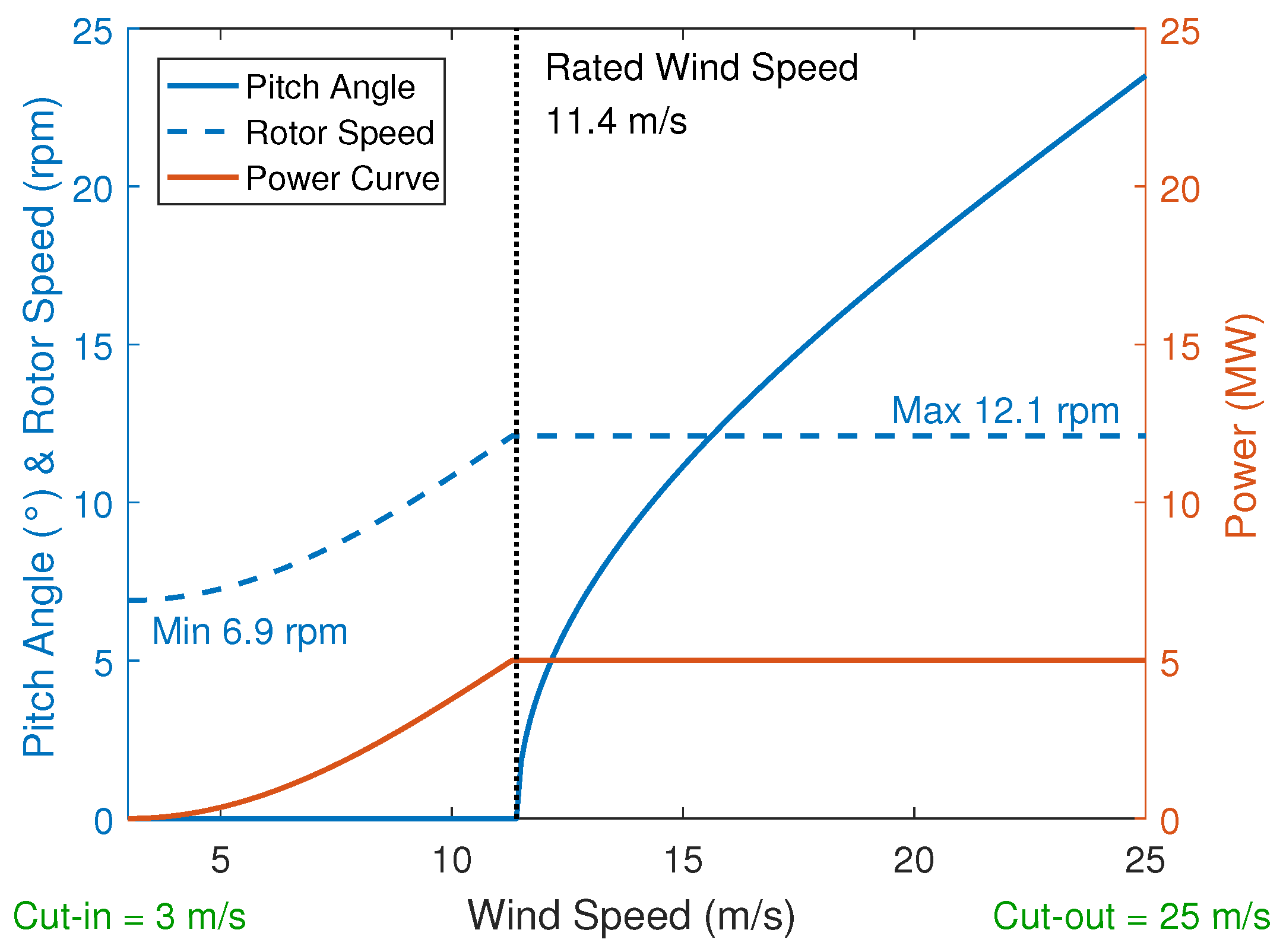
Figure 5.
Filled contours of wind speed over vertical cross-sections at the center of the computational domain ( km) for downburst winds in three cases: (a) C1-0x0y, (b) N-0x0y and (c) S2-0x0y (snapshots of the wind fields are taken at 450 s). The vertical dashed line denotes the location of wind turbines considered (i.e., at km). The color bar denotes the magnitude of the full 3-D velocity; the arrows denote the direction projected onto the x-z plane (the arrow lengths also convey the velocity magnitude, as indicated).

Figure 6.
Filled contours of wind speed over a horizontal plane at hub height for downburst winds in three cases: (a) C1-0x0y, (b) N-0x0y and (c) S2-0x0y (snapshots of the wind fields are taken at 600 s). The vertical dashed line denotes the location of turbines considered (i..e, at km). The color bar denotes the magnitude of the full 3-D velocity; the arrows denote the direction projected onto the x-y plane (the arrow lengths also convey the velocity magnitude, as indicated).
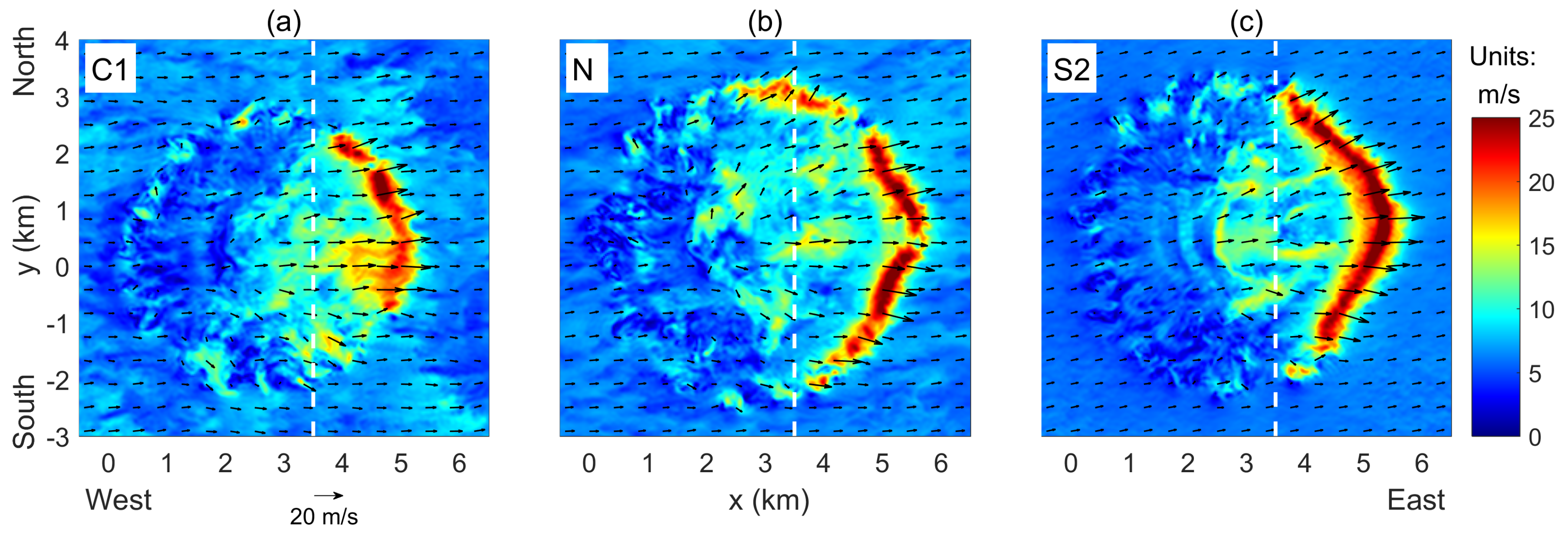
Figure 7.
Hub-height velocity time series (all three components) for the selected case, 0x0y-X1, and for all the five atmospheric stability conditions. A 25-s moving average window is applied to the data.
Figure 7.
Hub-height velocity time series (all three components) for the selected case, 0x0y-X1, and for all the five atmospheric stability conditions. A 25-s moving average window is applied to the data.

Figure 8.
Summary statistics on the three velocity components (, and ) and on the wind direction change (WndDir) at hub height in Periods I, II and III during the downburst simulations. Ramp rate statistics in Period II are related to the primary surge in . All data from the 120 generated wind fields are used (24 samples are used for the error bars, which represent one standard deviation on either side of the mean).
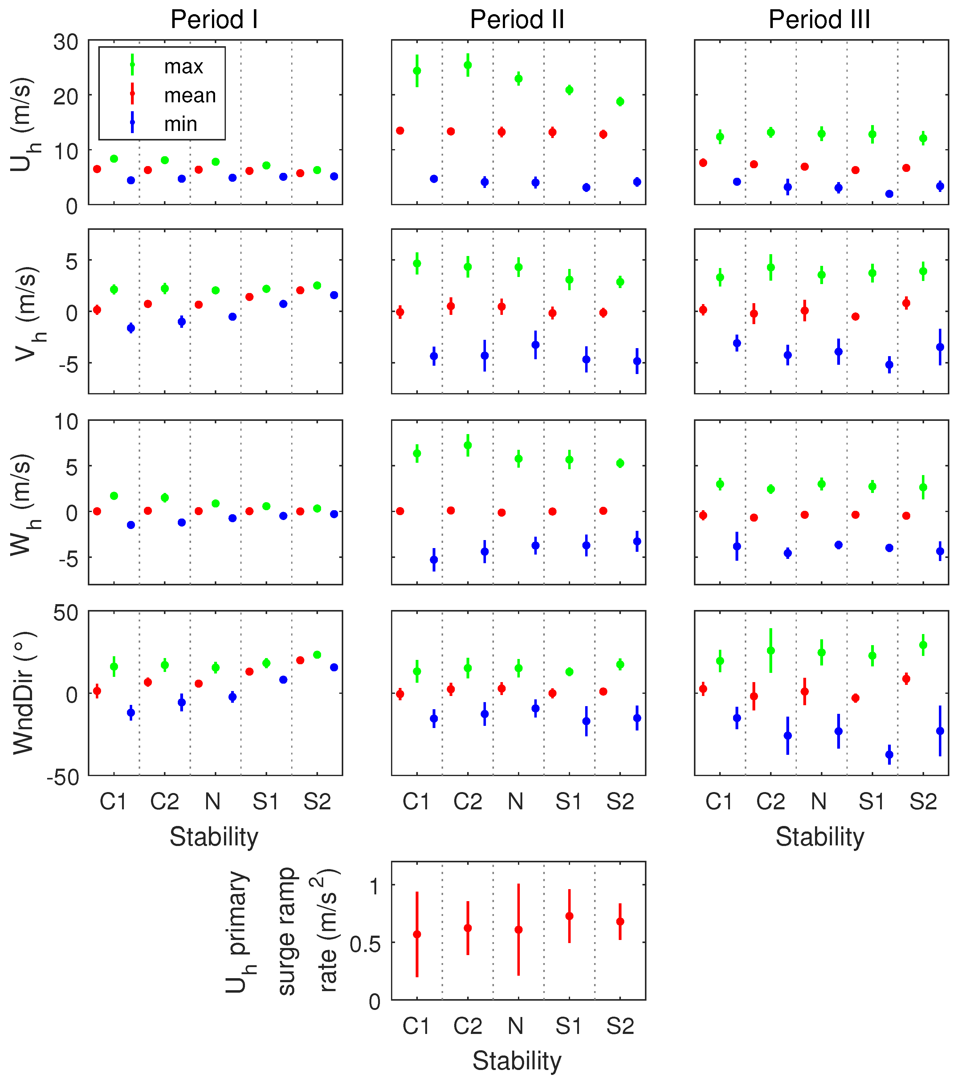
Figure 9.
Hub-height velocity time series (all three components) for cases C1-X1 and S2-X1 with four different initial locations of downburst cooling source.
Figure 9.
Hub-height velocity time series (all three components) for cases C1-X1 and S2-X1 with four different initial locations of downburst cooling source.

Figure 10.
Hub-height velocity time series (all three components) for cases C1-0x0y and S2-0x0y with six different turbine locations, X1–X6.
Figure 10.
Hub-height velocity time series (all three components) for cases C1-0x0y and S2-0x0y with six different turbine locations, X1–X6.

Figure 11.
Time series of the hub-height horizontal wind speed (), the hub-height vertical wind speed (), the blade pitch angle (PitAng), the hub-height wind direction (), the nacelle yaw angle (YawAng), the yaw error (YawErr) and three turbine loads (OoPBM, FATBM and TTYM) for a selected single case, N-0x0y-X1. The red diamond markers denote extreme values.

Figure 12.
Time series of OoPBM, FATBM, and TTYM for the selected case, 0x0y-X1, and five different atmospheric stability conditions. A 25-s moving average window is applied to the data.
Figure 12.
Time series of OoPBM, FATBM, and TTYM for the selected case, 0x0y-X1, and five different atmospheric stability conditions. A 25-s moving average window is applied to the data.
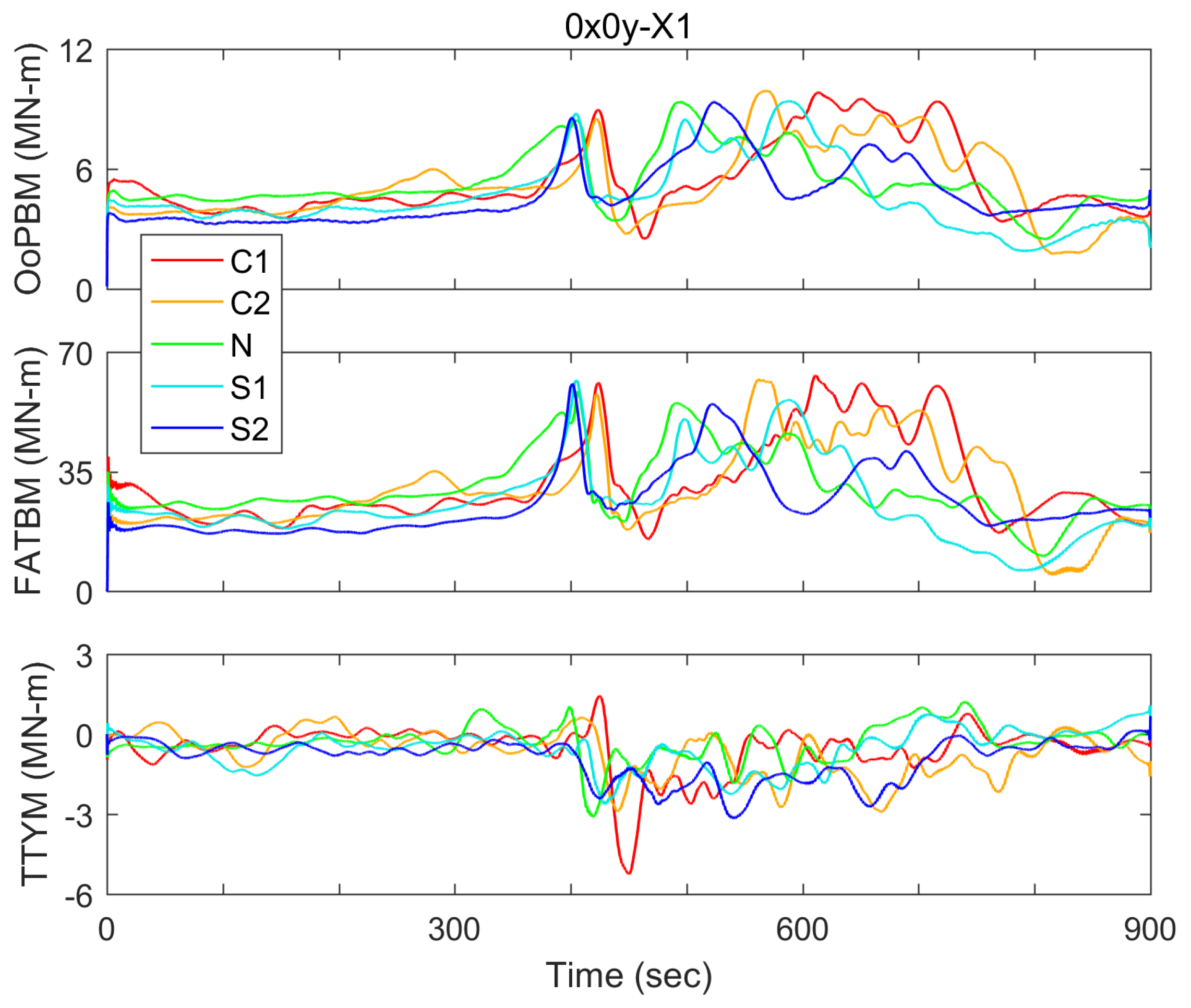
Figure 13.
Histograms of turbine load ranges, obtained using rainflow cycle-counting, for the C1, N and S2 cases (selected wind fields are for the case, 0x0y-X1).
Figure 13.
Histograms of turbine load ranges, obtained using rainflow cycle-counting, for the C1, N and S2 cases (selected wind fields are for the case, 0x0y-X1).

Figure 14.
Time series of OoPBM, FATBM, and TTYM for the cases, C1-X1 and S2-X1, with four different initial locations of the downburst cooling source. A 25-s moving average window is applied to the data.
Figure 14.
Time series of OoPBM, FATBM, and TTYM for the cases, C1-X1 and S2-X1, with four different initial locations of the downburst cooling source. A 25-s moving average window is applied to the data.

Figure 15.
Time series of OoPBM, FATBM, and TTYM for the cases, C1-0x0y and S2-0x0y, with six different turbine locations. A 25-s moving average window is applied to the data.
Figure 15.
Time series of OoPBM, FATBM, and TTYM for the cases, C1-0x0y and S2-0x0y, with six different turbine locations. A 25-s moving average window is applied to the data.

Figure 16.
Examples of four scenarios that indicate the occurrence of peak values in the OoPBM time series during the downburst. The peak values are denoted by diamond markers. Time series for the horizontal wind speed (blue) and blade pitch angle (red) are shown.
Figure 16.
Examples of four scenarios that indicate the occurrence of peak values in the OoPBM time series during the downburst. The peak values are denoted by diamond markers. Time series for the horizontal wind speed (blue) and blade pitch angle (red) are shown.

Figure 17.
Time series of the hub-height horizontal wind speed (), the blade pitch angle (PitAng), and turbine loads for the C1, N and S2 cases showing various scenarios for extreme load occurrence. Wind fields for 5x5y-X6 are selected for illustration.
Figure 17.
Time series of the hub-height horizontal wind speed (), the blade pitch angle (PitAng), and turbine loads for the C1, N and S2 cases showing various scenarios for extreme load occurrence. Wind fields for 5x5y-X6 are selected for illustration.

Figure 18.
Filled contours of velocity: (a) at the turbine hub height; and (b) on the center (vertical) line of the rotor plane for the 0x0y-X1 C1, N, and S2 cases. The arrows represent wind direction projected onto relevant planes for each figure. The occurrence times for extreme values of OoPBM, FATBM and TTYM are denoted by the letters of O, F and T, respectively.

Figure 19.
Filled contours of velocity of selected turbine-scale fields on vertical y-z planes through the rotor center: (1) at s; and (2) at the occurrence times of the extreme OoPBM, FATBM and TTYM loads. Wind fields from the 0x0y-X1 case are selected. The color bar applied to the velocity. The arrows represent velocity projected onto the y-z plane.
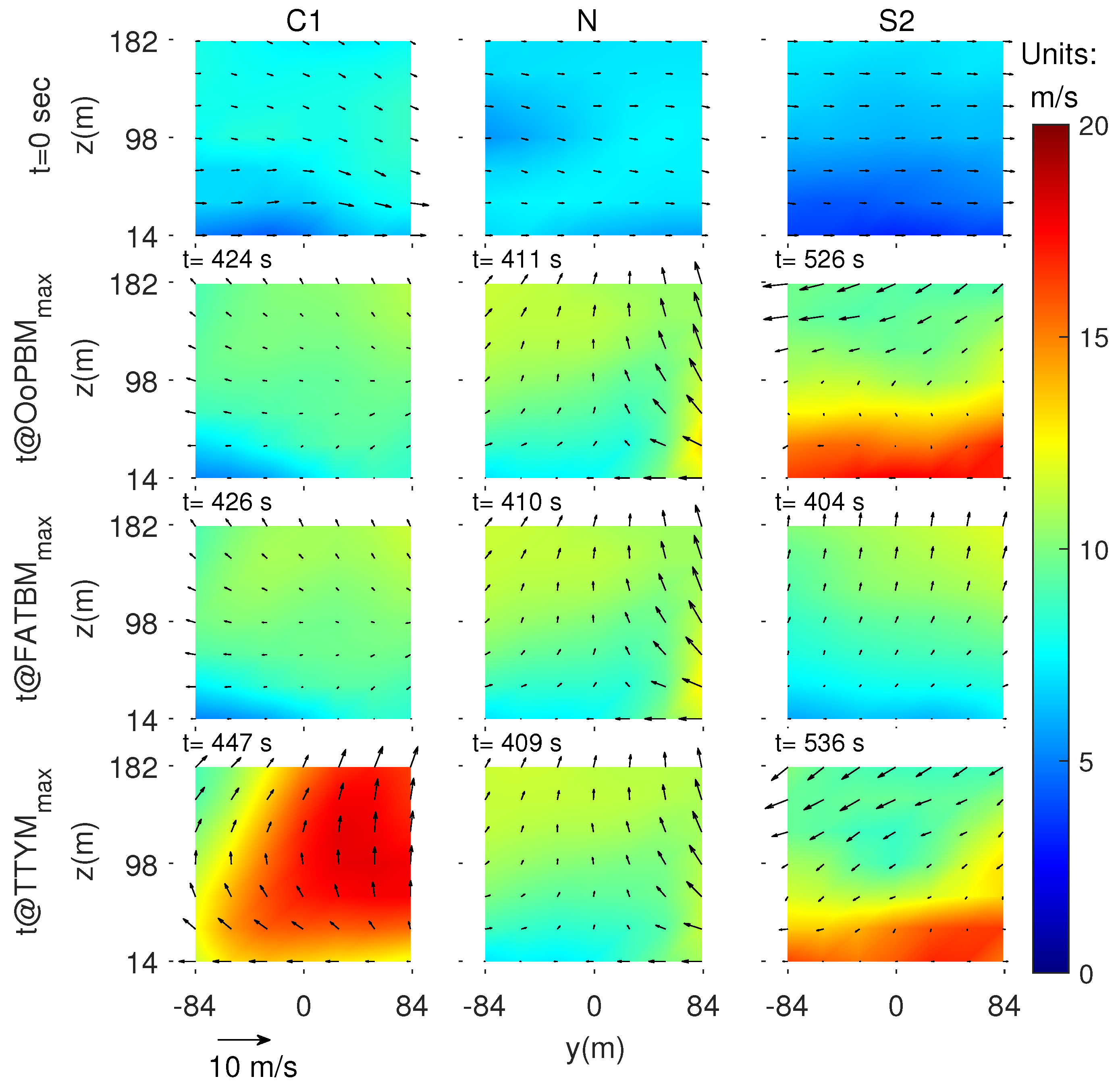
Figure 20.
Box plots of equivalent fatigue load (EFL) and extreme load (ExL) statistics for different atmospheric stabilities (24 samples are used for each stability case).
Figure 20.
Box plots of equivalent fatigue load (EFL) and extreme load (ExL) statistics for different atmospheric stabilities (24 samples are used for each stability case).
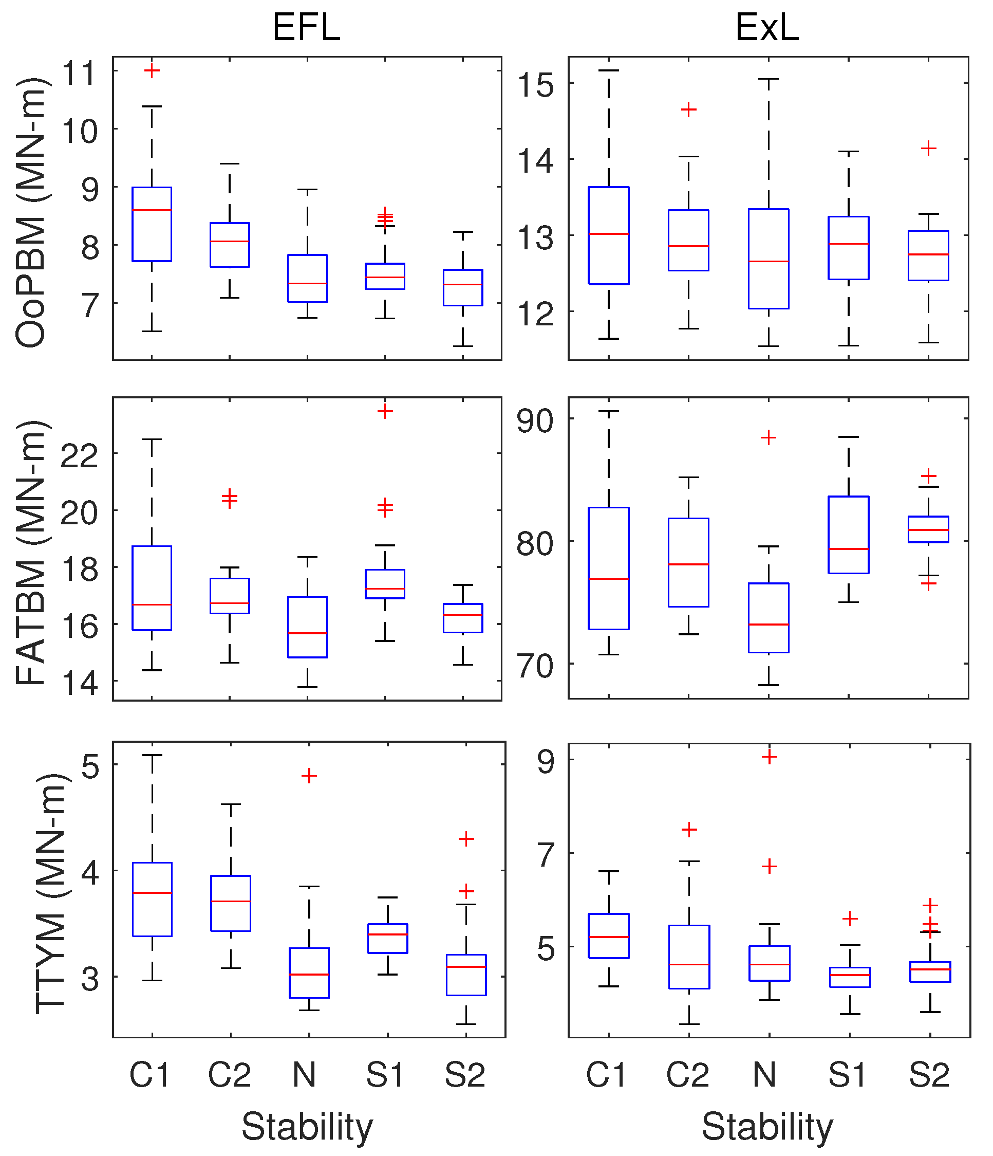
Figure 21.
Comparison of the ratio of maximum loads in Periods II-III to those in Period I for a selected turbine location, X1, and for five different stability cases. Samples with four different cooling source locations are denoted by different markers.
Figure 21.
Comparison of the ratio of maximum loads in Periods II-III to those in Period I for a selected turbine location, X1, and for five different stability cases. Samples with four different cooling source locations are denoted by different markers.


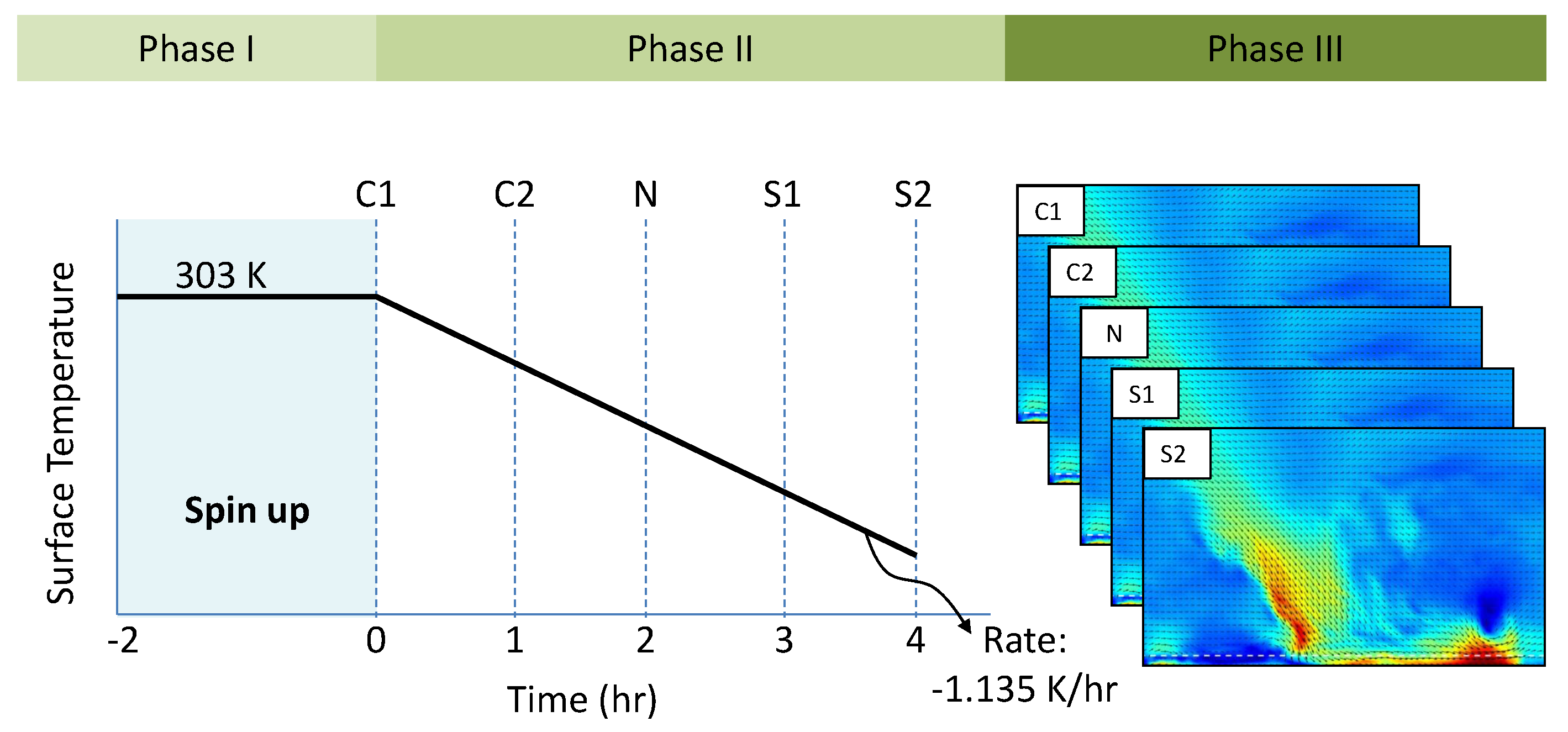
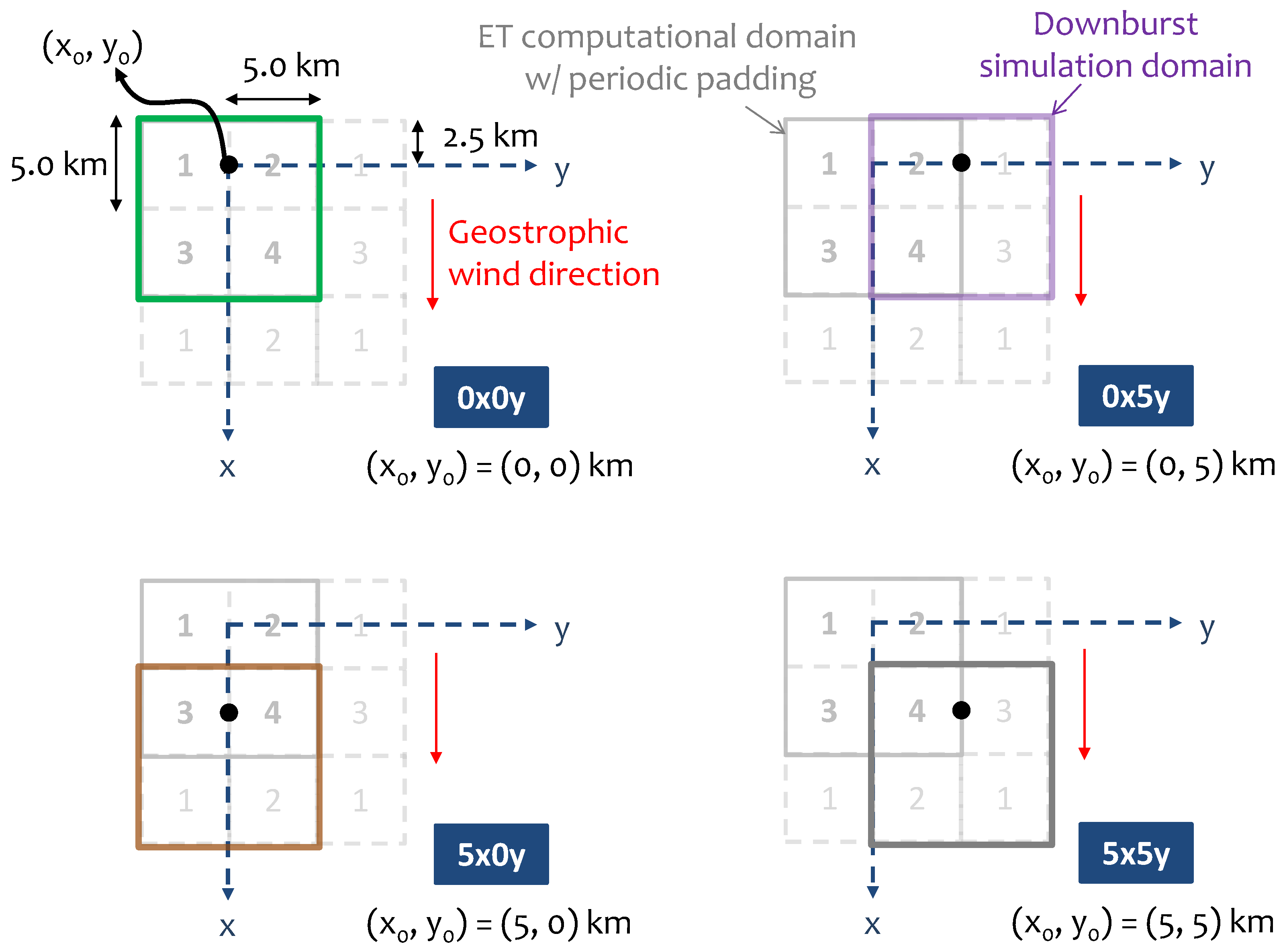
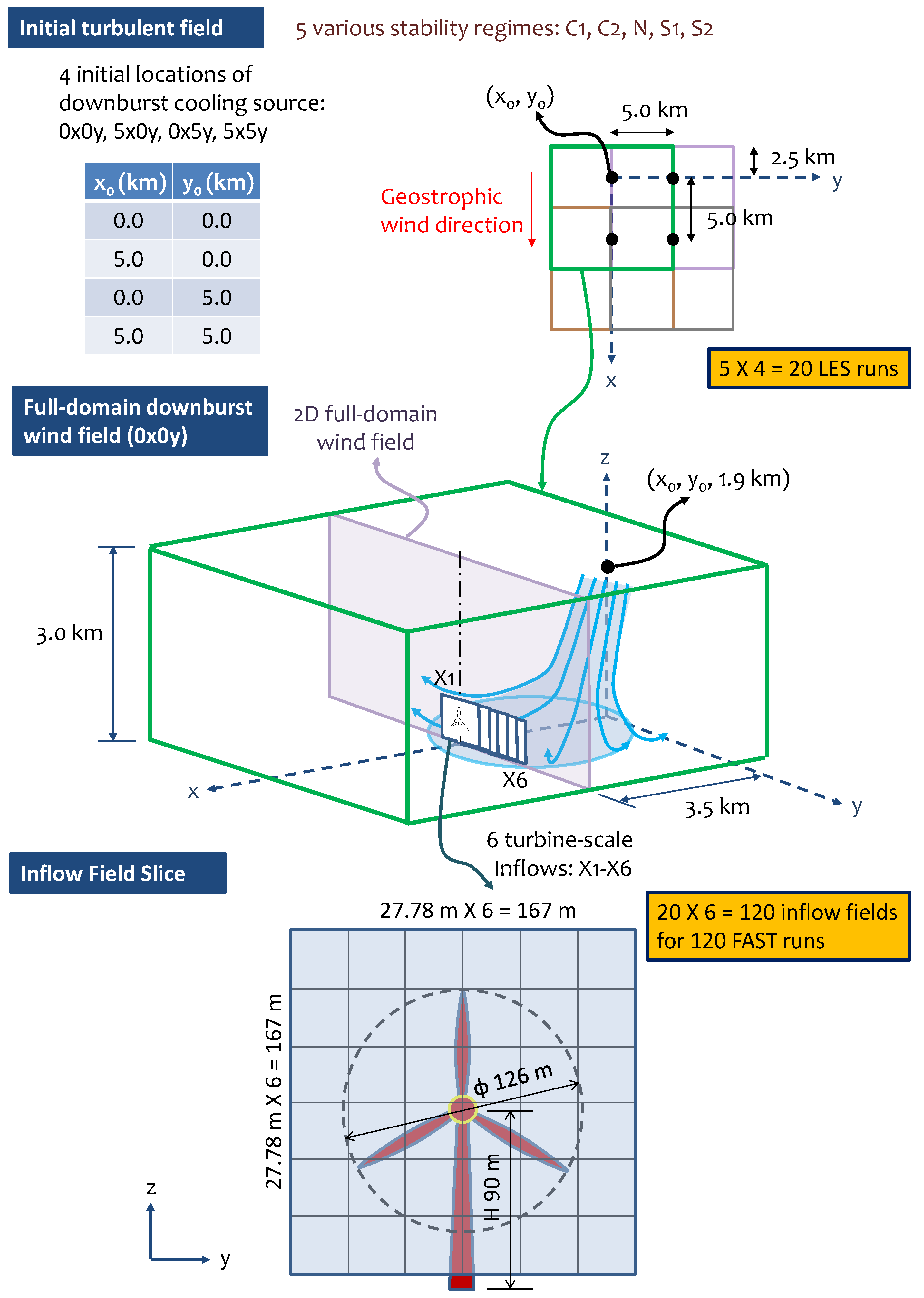
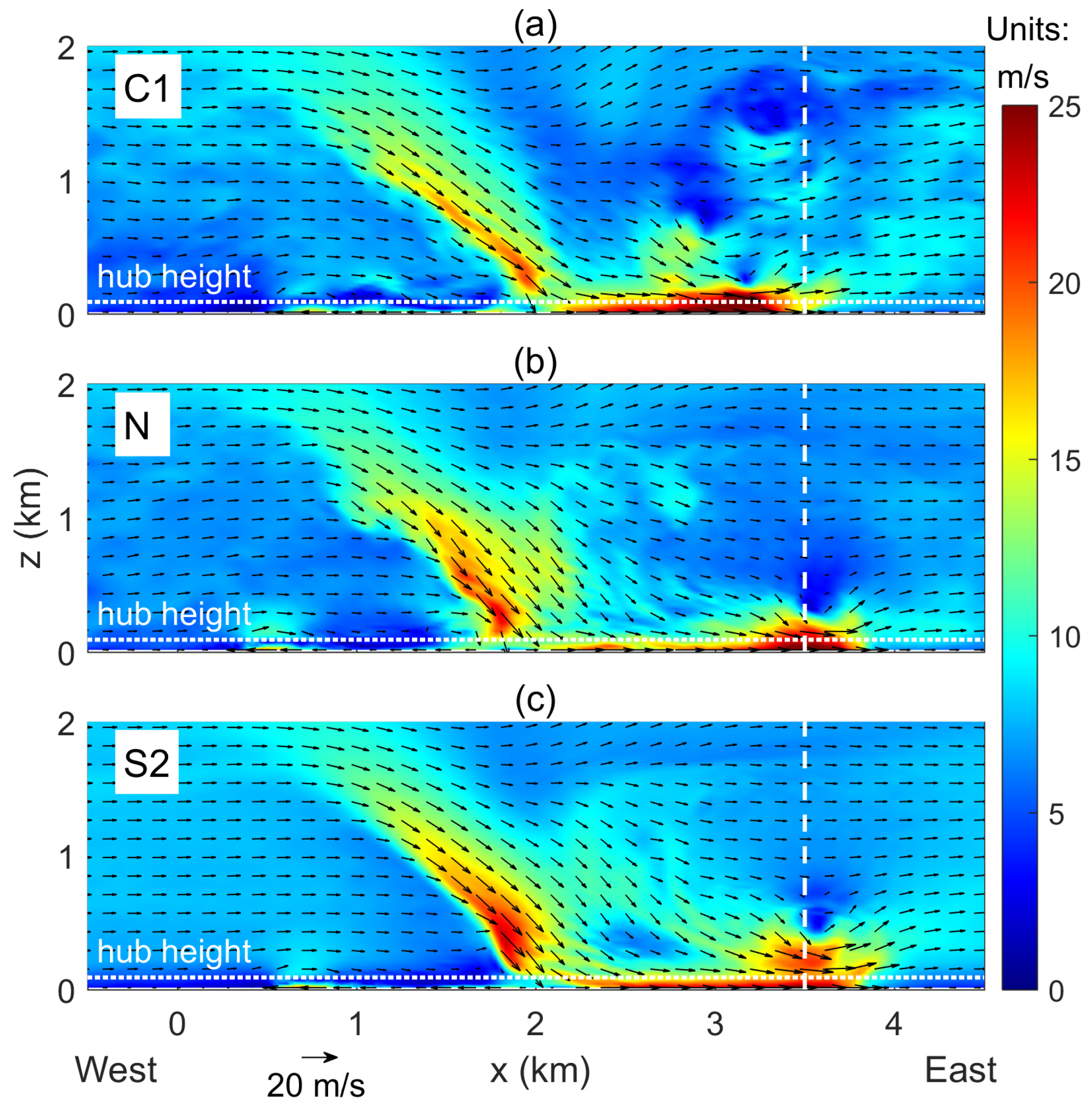
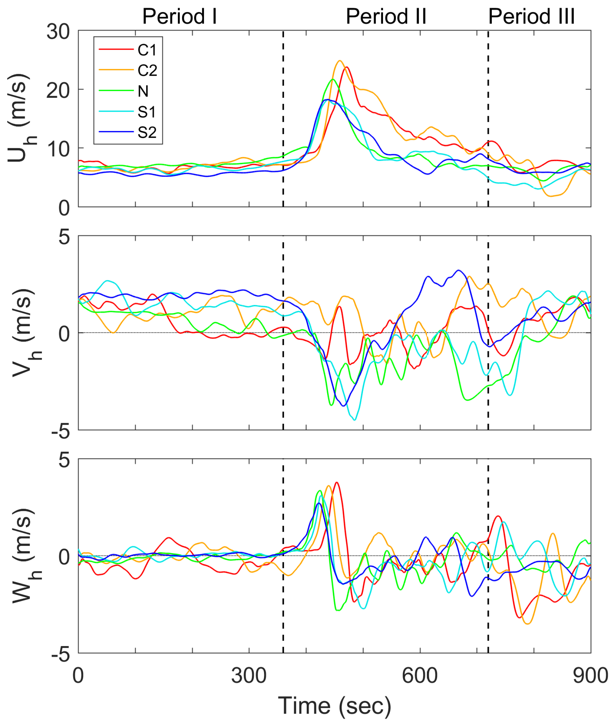
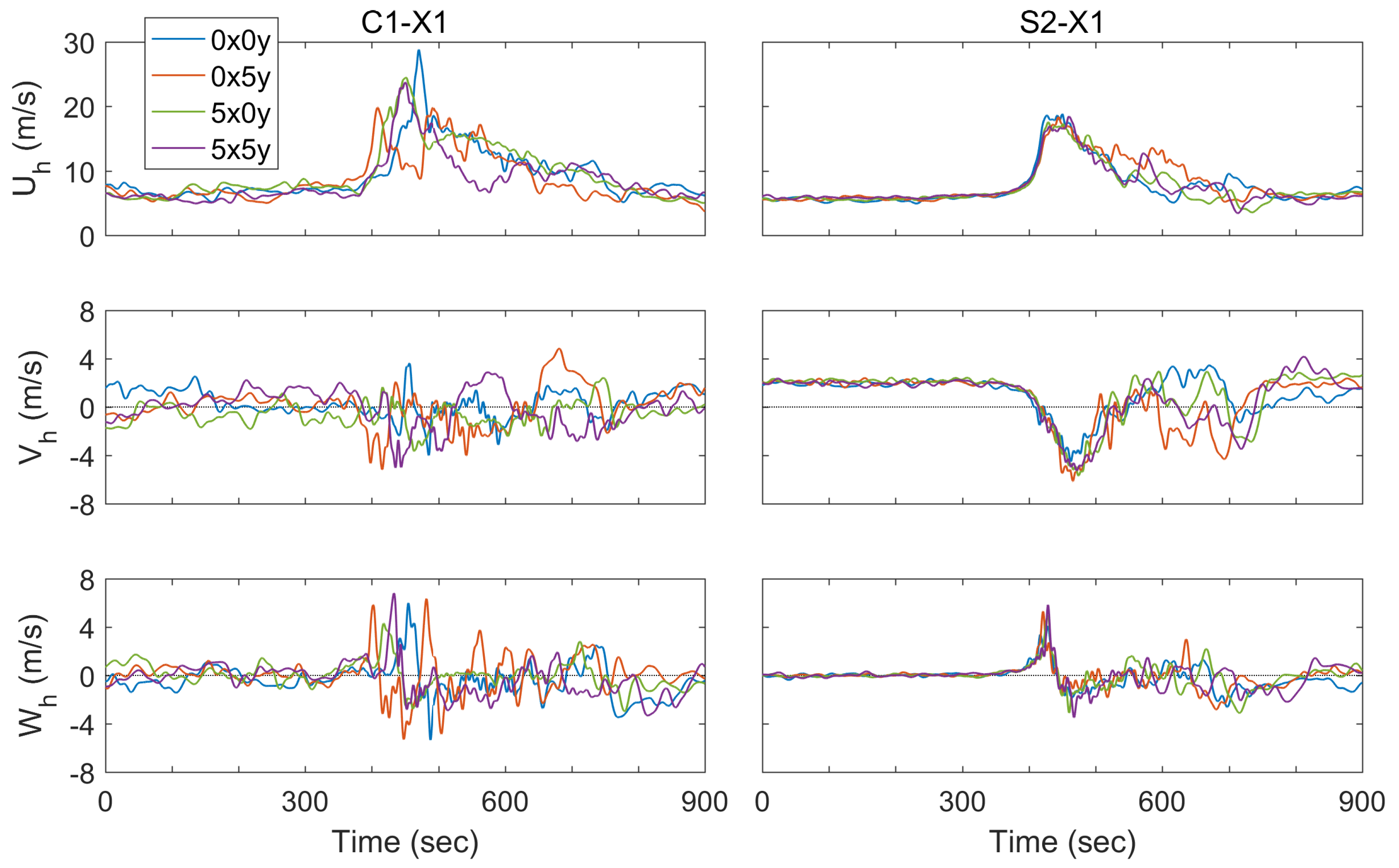
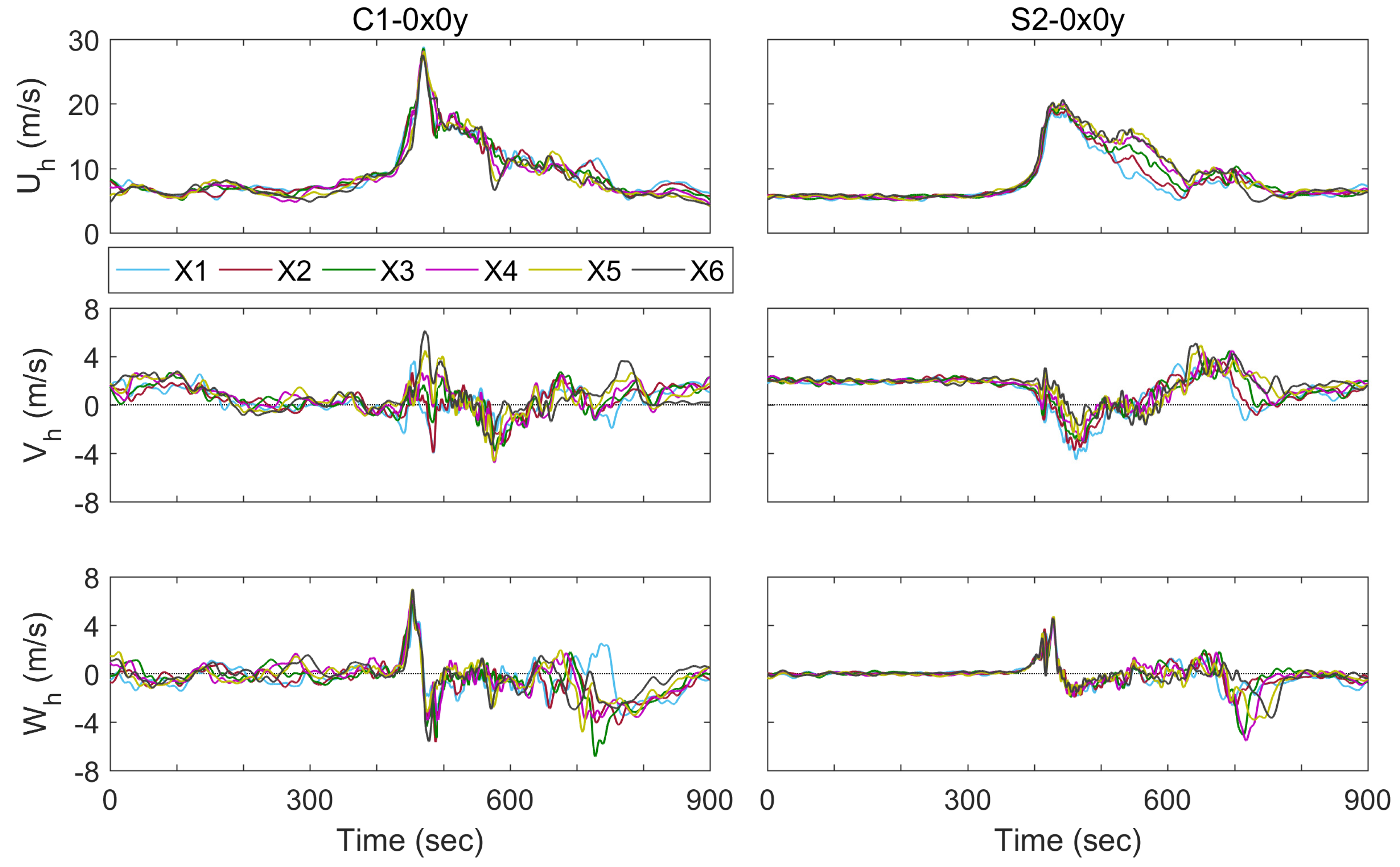
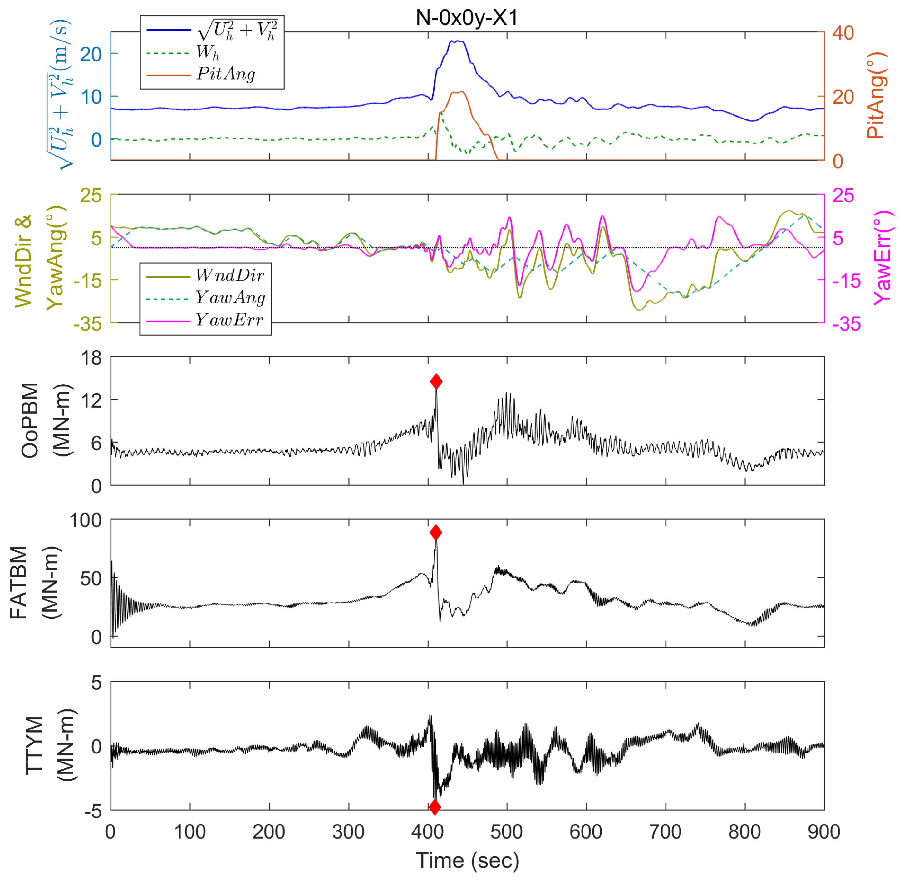
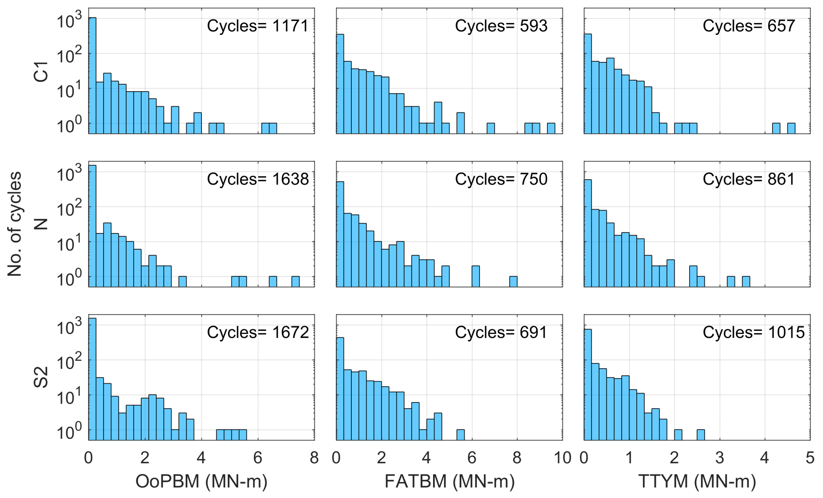
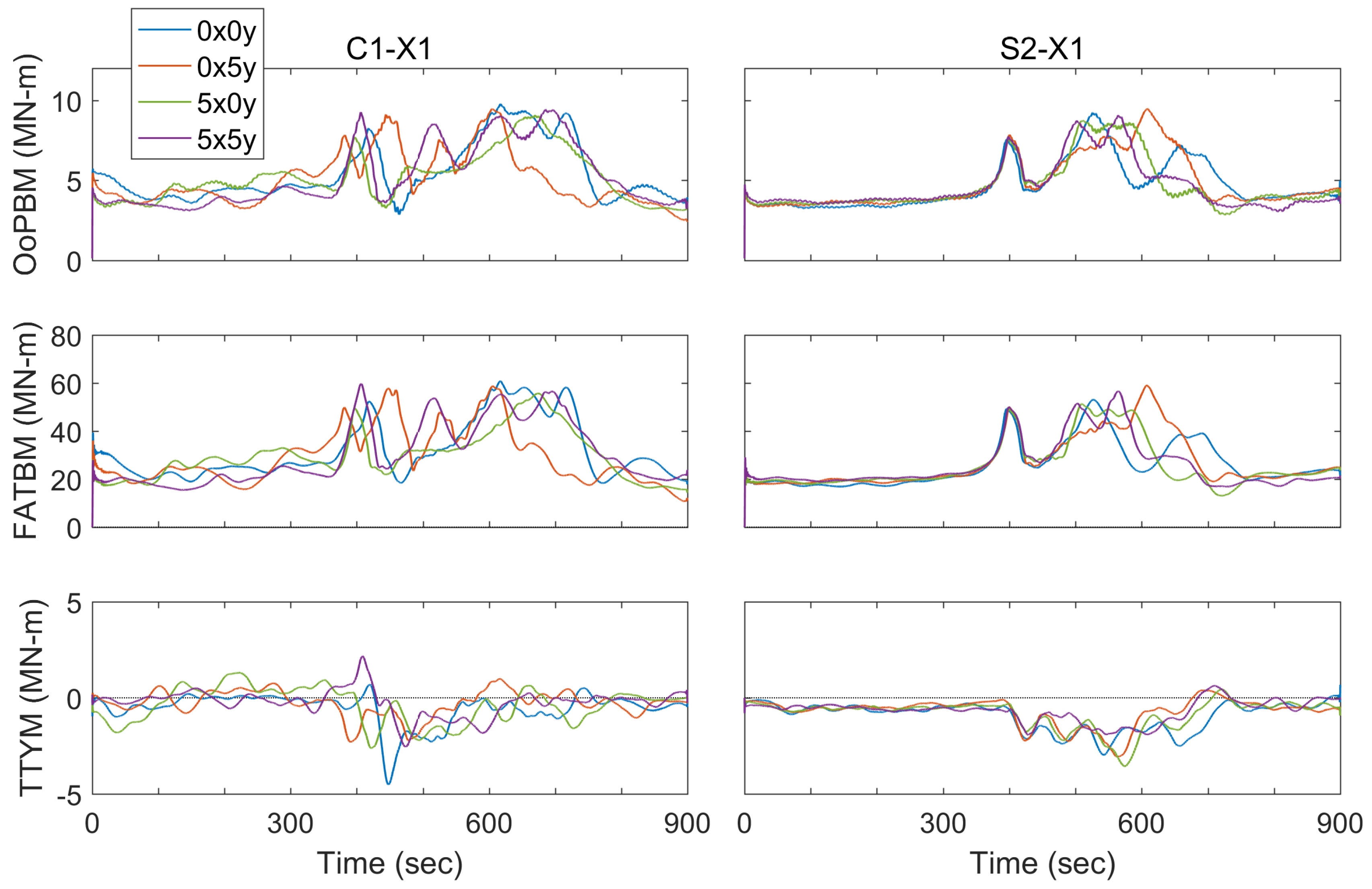
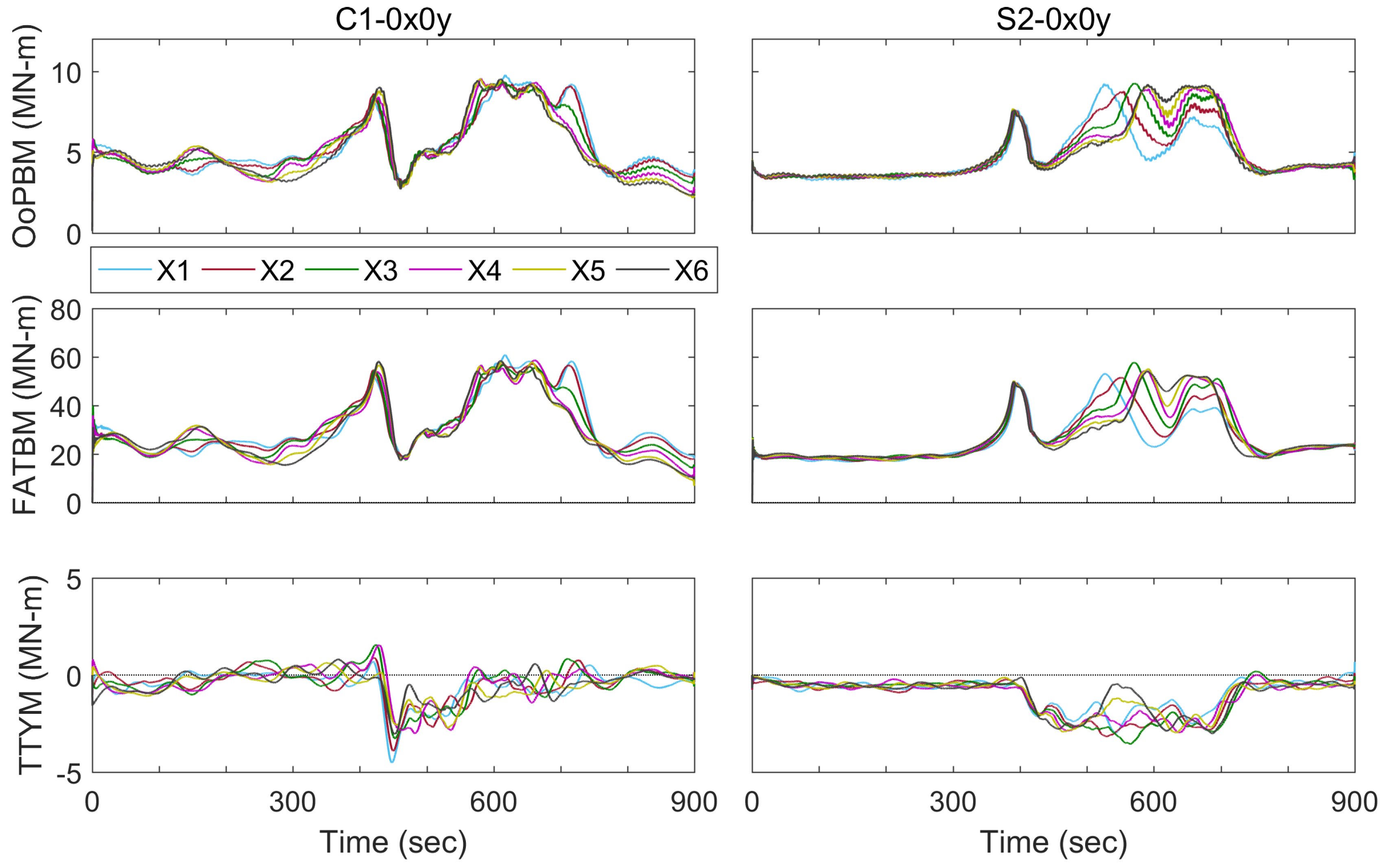
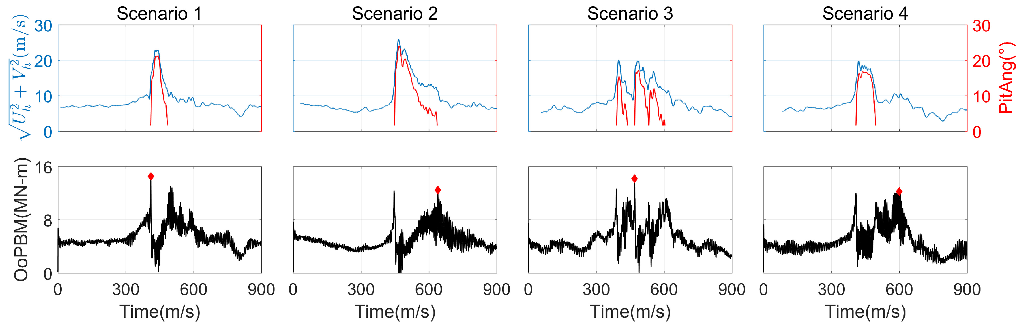
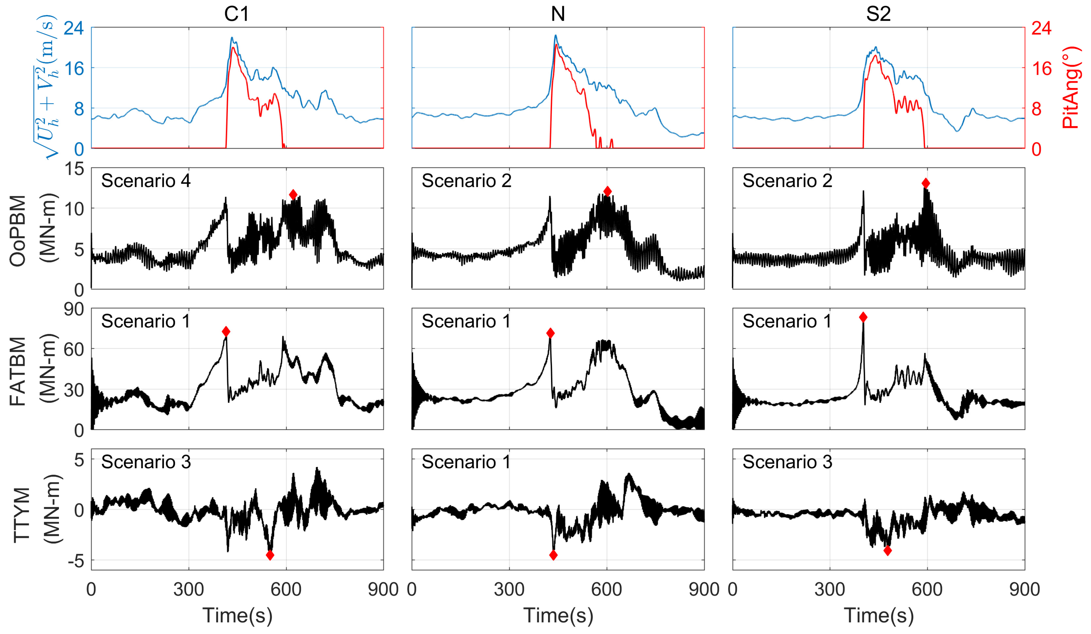
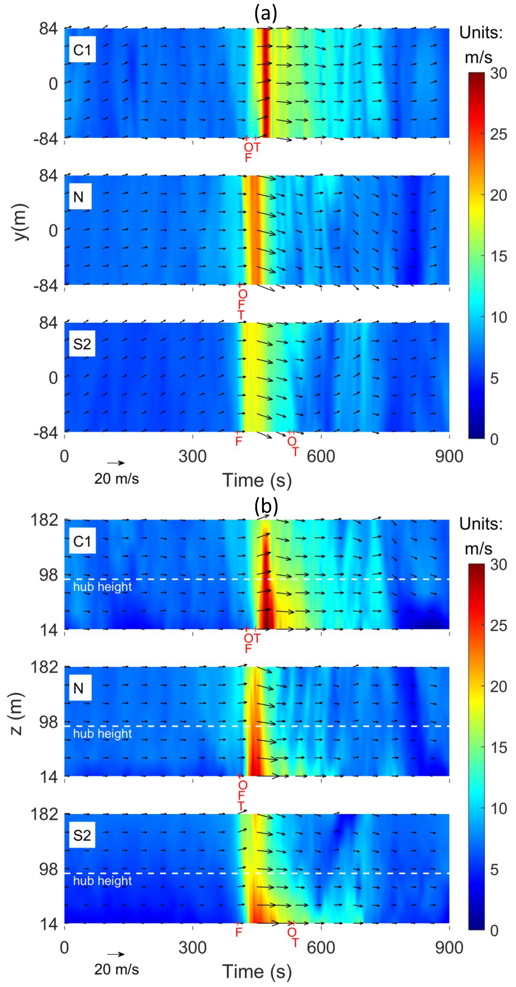
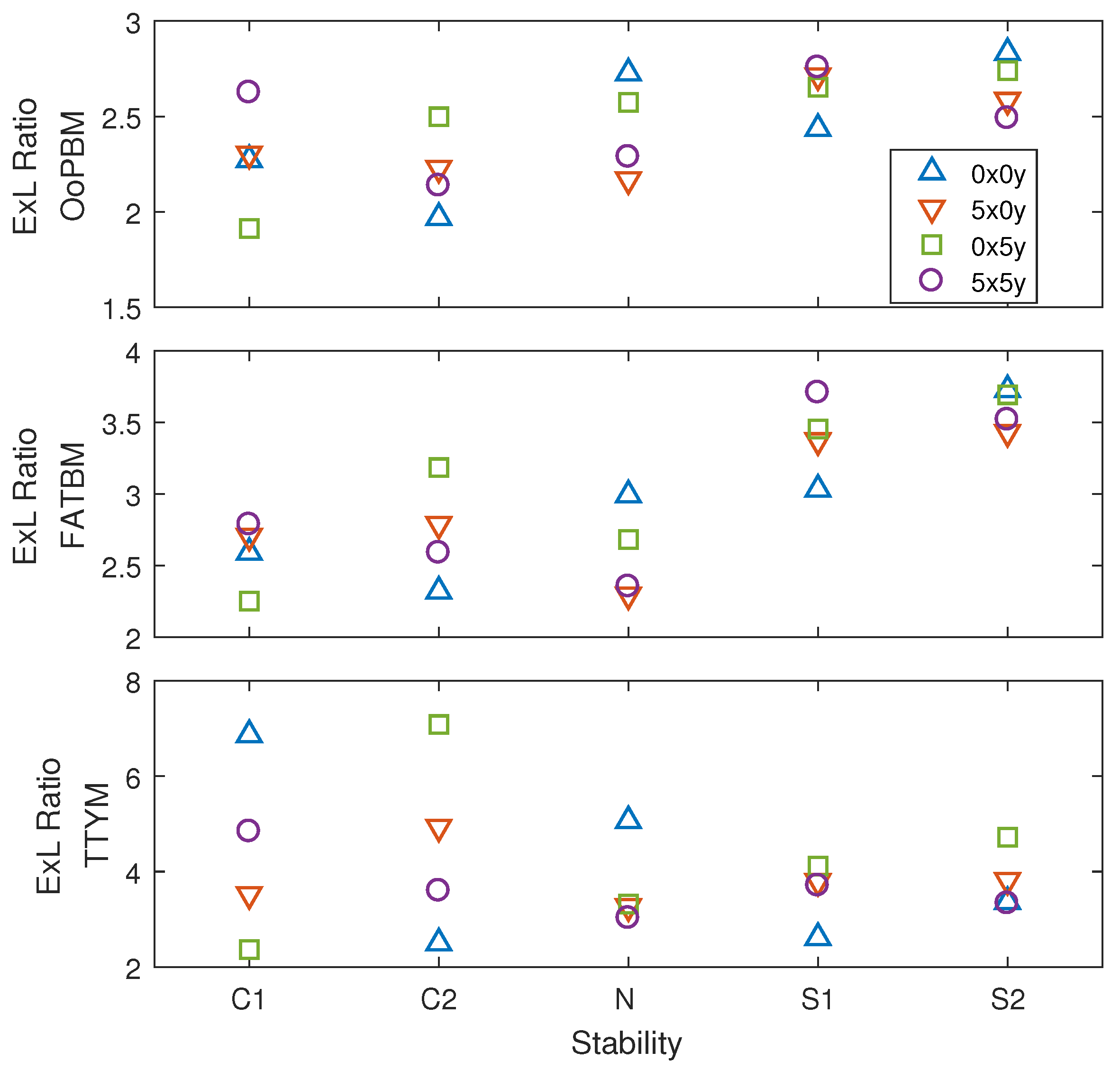
Table 1.
Properties and dimensions of the 5-MW NREL turbine model.
| Properties and Dimensions | Values |
|---|---|
| Power rating | 5 MW |
| Rotor type | Upwind/ 3-bladed |
| Rotor diameter | 126 m |
| Hub height | 90 m |
| Cut-in, rated, cut-out speed | 3, 11.4, 25 m/s |
| rated rotor speed | 12.1 rpm |
| Rotor mass | 110,000 kg |
| Nacelle mass | 240,000 kg |
| Tower mass | 347,460 kg |
Table 2.
List of all the LES runs used in this study.
| No. | Stability | Downburst Initial Location |
|---|---|---|
| 1 | C1 | 0x0y |
| 2 | C1 | 5x0y |
| 3 | C1 | 0x5y |
| 4 | C1 | 5x5y |
| 5 | C2 | 0x0y |
| 6 | C2 | 5x0y |
| 7 | C2 | 0x5y |
| 8 | C2 | 5x5y |
| 9 (control) | N | 0x0y |
| 10 | N | 5x0y |
| 11 | N | 0x5y |
| 12 | N | 5x5y |
| 13 | S1 | 0x0y |
| 14 | S1 | 5x0y |
| 15 | S1 | 0x5y |
| 16 | S1 | 5x5y |
| 17 | S2 | 0x0y |
| 18 | S2 | 5x0y |
| 19 | S2 | 0x5y |
| 20 | S2 | 5x5y |
| Wind Speed | Wind Ramp Rate | Wind Dir. | Wind Dir. Chg. | Yaw | OoPBM | OoPBM | TTYM | |
|---|---|---|---|---|---|---|---|---|
| Max. (m/s) | Max. (m/s) | Change (deg) | Rate (deg/s) | Control? | ExL (MN-m) | EFL (MN-m) | ExL (MN-m) | |
| Case 3b | 55.0 | 1.0 | 110.0 | 1.2 | Yes | 22.5 | / | 26.8 |
| Nguyen et al. [10] | ||||||||
| Case 2 | ~32.0 | / | ~63.0 | / | Yes | 12.3 | 6.9 | / |
| Nguyen and Manuel [13] | ||||||||
| Present Study | 28.8 | 1.6 | 21.3 | 4.8 | Yes | 11.7 | 8.1 | 6.6 |
| C1-0x0y-X1 |
© 2019 by the authors. Licensee MDPI, Basel, Switzerland. This article is an open access article distributed under the terms and conditions of the Creative Commons Attribution (CC BY) license (http://creativecommons.org/licenses/by/4.0/).
Share and Cite
MDPI and ACS Style
Lu, N.-Y.; Hawbecker, P.; Basu, S.; Manuel, L. On Wind Turbine Loads During Thunderstorm Downbursts in Contrasting Atmospheric Stability Regimes. Energies 2019, 12, 2773. https://doi.org/10.3390/en12142773
AMA Style
Lu N-Y, Hawbecker P, Basu S, Manuel L. On Wind Turbine Loads During Thunderstorm Downbursts in Contrasting Atmospheric Stability Regimes. Energies. 2019; 12(14):2773. https://doi.org/10.3390/en12142773
Chicago/Turabian StyleLu, Nan-You, Patrick Hawbecker, Sukanta Basu, and Lance Manuel. 2019. "On Wind Turbine Loads During Thunderstorm Downbursts in Contrasting Atmospheric Stability Regimes" Energies 12, no. 14: 2773. https://doi.org/10.3390/en12142773
Note that from the first issue of 2016, this journal uses article numbers instead of page numbers. See further details here.