Impacts of Climate Change and Climate Variability on Hydropower Potential in Data-Scarce Regions Subjected to Multi-Decadal Variability


Abstract
:1. Introduction
2. Study Area
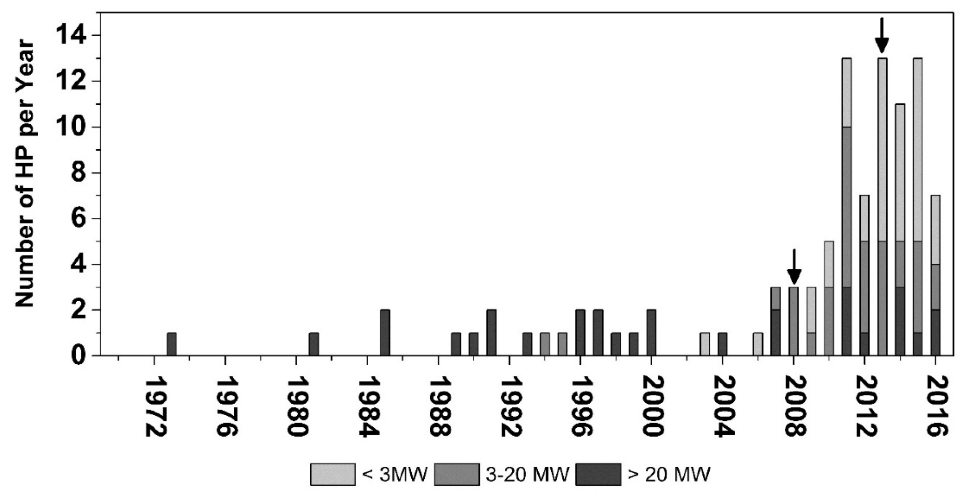
2.1. Hydropower Development in Chile
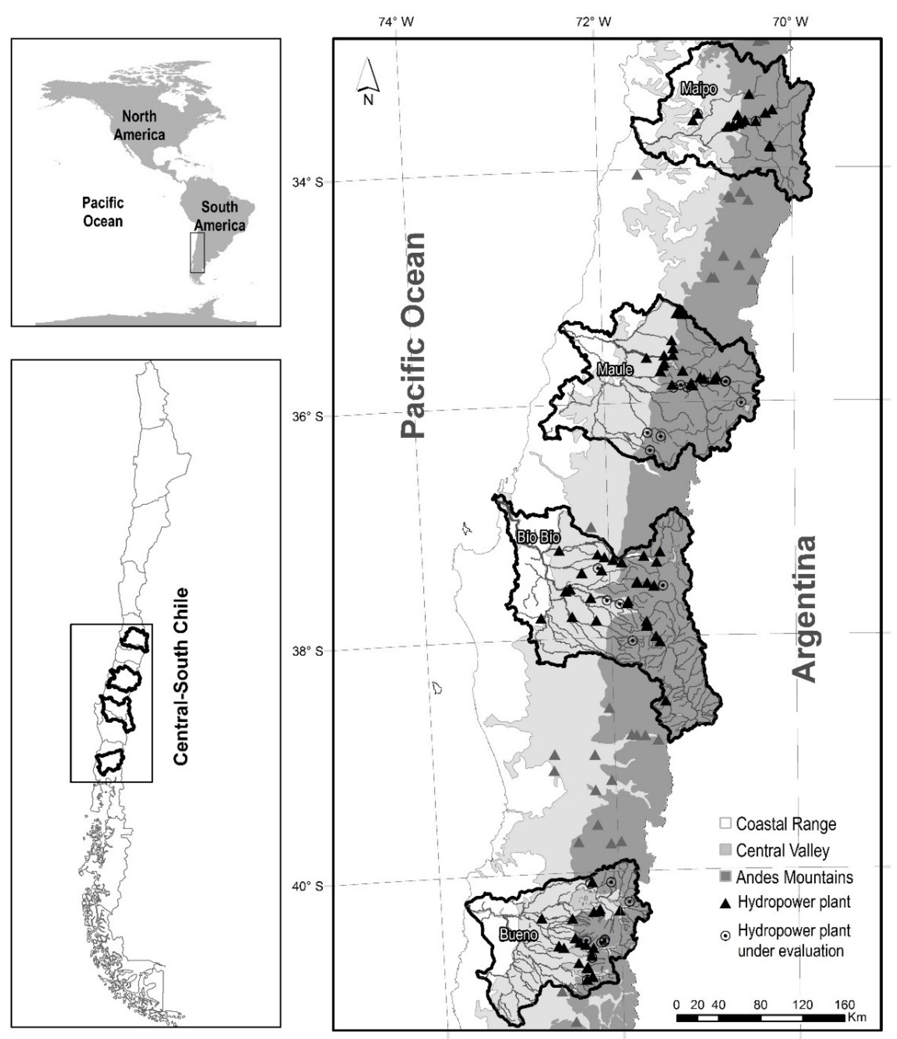
2.2. Study Basins
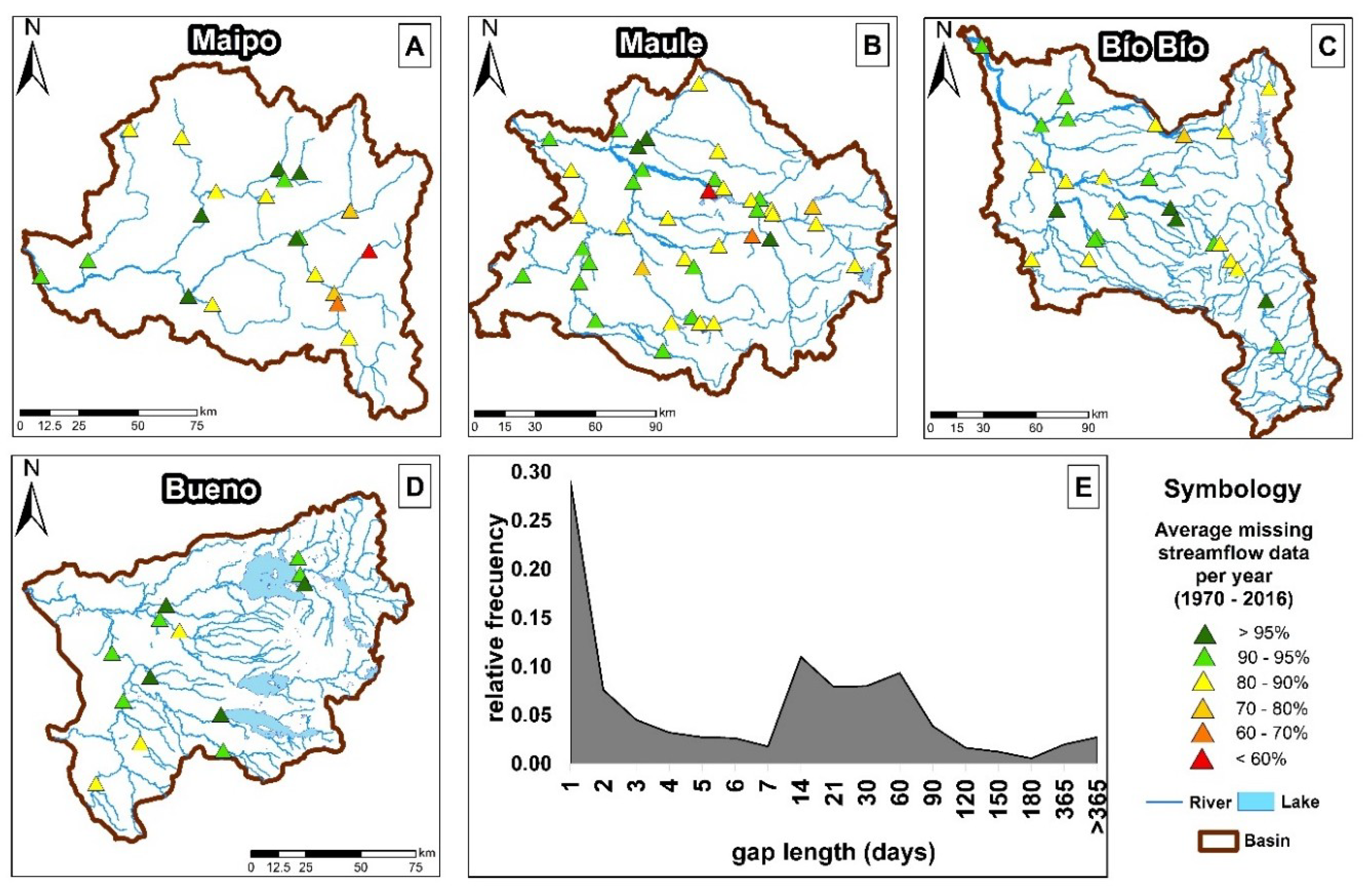
Streamflow Data
3. Methods
3.1. Gap Filling Method
3.2. Historical Hydropower Potential
Estimation of Discharge in Each River Reach
3.3. Trends in Hydropower Potential
3.4. Correlation between Hydropower Potential and Long-Term Climate Variability
3.5. Developing Future Scenarios for Hydropower Potential Amid Climate Change
4. Results and Discussion
4.1. Gap-Filling Perfomance
4.2. Hydropower Potential Variability and Trends
4.3. Correlation between Hydropower Potential and Long-Term Climate Variability
4.4. Future Scenarios for Hydropower Amid Climate Change
5. Conclusions
Supplementary Materials
Author Contributions
Funding
Acknowledgments
Conflicts of Interest
References
- International Energy Agency. Energy Statistics; International Energy Agency: Paris, France, 2018. [Google Scholar]
- Barros, R.M.; Tiago Filho, G.L. Small hydropower and carbon credits revenue for an SHP project in national isolated and interconnected systems in Brazil. Renew. Energy 2012, 48, 27–34. [Google Scholar] [CrossRef]
- Zarfl, C.; Lumsdon, A.E.; Tockner, K. A global boom in hydropower dam construction. Aquat. Sci. 2015, 77, 161–170. [Google Scholar] [CrossRef]
- Killingtveit, A. Hydropower. In Managing Global Warmimng; Elsevier: Amsterdam, The Netherlands, 2019; pp. 265–315. [Google Scholar]
- Zhou, Y.; Hejazi, M.; Smith, S.; Edmonds, J.; Li, H.; Clarke, L.; Calvin, K.; Thomson, A. A comprehensive view of global potential for hydrogenerated electricity. Energy Environ. Sci. 2015, 8, 2622–2633. [Google Scholar] [CrossRef]
- Zhang, X.; Li, H.Y.; Deng, Z.D.; Ringler, C.; Gao, Y.; Hejazi, M.I.; Leung, L.R. Impacts of climate change, policy and Water-Energy-Food nexus on hydropower development. Renew. Energy 2018, 116, 827–834. [Google Scholar] [CrossRef]
- Van Vliet, M.T.H.; Wiberg, D.; Leduc, S.; Riahi, K. Power-generation system vulnerability and adaptation to changes in climate and water resources. Nat. Clim. Chang. 2016, 6, 375–380. [Google Scholar] [CrossRef]
- Engeland, K.; Borga, M.; Creutin, J.-D.; François, B.; Ramos, M.-H.; Vidal, J.-P. Space-time variability of climate variables and intermittent renewable electricity production—A review. Renew. Sustain. Energy Rev. 2017, 79, 600–617. [Google Scholar] [CrossRef]
- Fabry, F. On the determination of scale ranges for precipitation fields. J. Geophys. Res. 1996, 101, 12819–12826. [Google Scholar] [CrossRef]
- Garreaud, R.D.; Vuille, M.; Compagnucci, R.; Marengo, J. Present-day South American climate. Palaeogeogr. Palaeoclimatol. Palaeoecol. 2009, 281, 180–195. [Google Scholar] [CrossRef]
- Ng, J.Y.; Turner, S.W.D.; Galelli, S. Influence of El Niño Southern Oscillation on global hydropower production. Environ. Res. Lett. 2017, 12, 034010. [Google Scholar] [CrossRef]
- Carvajal, P.E.; Anandarajah, G.; Mulugetta, Y.; Dessens, O. Assessing uncertainty of climate change impacts on long-term hydropower generation using the CMIP5 ensemble—The case of Ecuador. Clim. Chang. 2017, 144, 611–624. [Google Scholar] [CrossRef]
- Turner, S.W.D.; Hejazi, M.; Kim, S.H.; Clarke, L.; Edmonds, J. Climate impacts on hydropower and consequences for global electricity supply investment needs. Energy 2017, 141, 2081–2090. [Google Scholar] [CrossRef]
- Hu, Y.; Jin, X.; Guo, Y. Big data analysis for the hydropower development potential of ASEAN-8 based on the hydropower digital planning model. J. Renew. Sustain. Energy 2018, 10, 034502. [Google Scholar] [CrossRef]
- Hamududu, B.H.; Killingtveit, Å. Hydropower production in future climate scenarios; the case for the Zambezi River. Energies 2016, 9, 502. [Google Scholar] [CrossRef]
- Hamududu, B.H.; Killingtveit, Å. Hydropower production in future climate scenarios: The case fro Kwanza River, Angola. Energies 2016, 9, 363. [Google Scholar] [CrossRef]
- Devia, G.K.; Ganasri, B.P.; Dwarakish, G.S. A Review on Hydrological Models. Aquat. Procedia 2015, 4, 1001–1007. [Google Scholar] [CrossRef]
- Emerson, D.G.; Vecchia, A.V.; Dahi, A.L. Evaluation of Drainage-Area Ratio Method Used to Estimate Streamflow for the Red River of the North Basin, North Dakota and Minnesota. Scientific Investigations Report 2005–5017 Evaluation of Drainage-Area Ratio Method Used to Estimate Streamflow for th. Sci. Investig. Rep. 2005. [Google Scholar] [CrossRef]
- Breiman, L. Random forests. Mach. Learn. 2001, 45, 5–32. [Google Scholar] [CrossRef]
- Stekhoven, D.J.; Bühlmann, P. Missforest-Non-parametric missing value imputation for mixed-type data. Bioinformatics 2012, 28, 112–118. [Google Scholar] [CrossRef]
- Chilkoti, V.; Bolisetti, T.; Balachandar, R. Climate change impact assessment on hydropower generation using multi-model climate ensemble. Renew. Energy 2017, 109, 510–517. [Google Scholar] [CrossRef]
- Comision Nacional de Energía Estadísticas electricidad en Chile. Available online: https://www.cne.cl/estadisticas/electricidad/ (accessed on 18 March 2019).
- Pollitt, M.G. Electricity reform in Chile: Lessons for developing countries. J. Netw. Ind. 2004, 5, 221–262. [Google Scholar] [CrossRef]
- Infraestructura de Datos Espaciales, Ministerio de Energía de Chile. Available online: http://sig.minenergia.cl/sig-minen/moduloCartografico/composer/ (accessed on 2 January 2018).
- Potencial Hidroeléctrico de Chile. Available online: http://walker.dgf.uchile.cl/Explorador/DAANC/ (accessed on 2 January 2018).
- Liang, X.; Lettenmaier, D.P.; Wood, E.F.; Burges, J. A simple hydrologically based model of land surface water and energy fluxes for general circulation models. J. Geophys. Res. 1994, 99, 14415–14428. [Google Scholar] [CrossRef]
- Santana, C.; Falvey, M.; Ibarra, M.; García, M. Energías Renovables en Chile. El Potencial Eólico, Solar e Hidroeléctrico de Arica a Chiloé. 2014. Available online: http://www.minenergia.cl/archivos_bajar/Estudios/Potencial_ER_en_Chile_AC.pdf (accessed on 28 January 2018).
- Energía 2050: Política Energética de Chile. Available online: http://www.energia2050.cl/es/energia-2050/energia-2050-politica-energetica-de-chile/ (accessed on 26 October 2017).
- Mapoteca Digital de Chile. Available online: http://www.dga.cl/estudiospublicaciones/mapoteca/Paginas/default.aspx (accessed on 2 January 2018).
- Rioseco, R.; Tesser, C. Cartografía Interactiva de Los Climas de Chile. Available online: http://www7.uc.cl/sw_educ/geografia/cartografiainteractiva/index.htm (accessed on 15 January 2018).
- Centro de Ciencia del Clima y Resiliencia CR2 Explorador Climático. Available online: http://explorador.cr2.cl/ (accessed on 30 January 2018).
- Valdés-Pineda, R.; Pizarro, R.; García-Chevesich, P.; Valdés, J.B.; Olivares, C.; Vera, M.; Balocchi, F.; Pérez, F.; Vallejos, C.; Fuentes, R.; et al. Water governance in Chile: Availability, management and climate change. J. Hydrol. 2014, 519, 2538–2567. [Google Scholar] [CrossRef]
- Sidibe, M.; Dieppois, B.; Mahé, G.; Paturel, J.E.; Amoussou, E.; Anifowose, B.; Lawler, D. Trend and variability in a new, reconstructed streamflow dataset for West and Central Africa, and climatic interactions, 1950–2005. J. Hydrol. 2018, 561, 478–493. [Google Scholar] [CrossRef]
- Moriasi, D.N.; Gitau, M.W.; Pai, N.; Daggupati, P. Hydrologic and Water Quality Models: Performance Measures and Evaluation Criteria. Trans. ASABE 2015, 58, 1763–1785. [Google Scholar] [Green Version]
- Kling, H.; Fuchs, M.; Paulin, M. Runoff conditions in the upper Danube basin under an ensemble of climate change scenarios. J. Hydrol. 2012, 424–425, 264–277. [Google Scholar] [CrossRef]
- U.S. Department of the Interior. U.S.G.S. Earth Explorer. Available online: https://earthexplorer.usgs.gov/ (accessed on 1 December 2017).
- Palla, A.; Gnecco, I.; La Barbera, P.; Ivaldi, M.; Caviglia, D. An Integrated GIS Approach to Assess the Mini Hydropower Potential. Water Resour. Manag. 2016, 30, 2979–2996. [Google Scholar] [CrossRef]
- Yousuf, I.; Ghumman, A.R.; Hashmi, H.N. Optimally sizing small hydropower project under future projected flows. KSCE J. Civ. Eng. 2017, 21, 1964–1978. [Google Scholar] [CrossRef]
- Mann, H.B. Nonparametric Tests Against Trend. Econometrica 1945, 13, 245–259. [Google Scholar] [CrossRef]
- Kendall, M.G. Rank Correlation Methods. Br. J. Stat. Psychol. 1956, 9, 68. [Google Scholar] [CrossRef]
- Yue, S.; Pilon, P.; Cavadias, G. Power of the Mann-Kendall and Spearman’s rho tests for detecting monotonic trends in hydrological series. J. Hydrol. 2002, 259, 254–271. [Google Scholar] [CrossRef]
- Kulkarni, A.; Storch, H. Von Monte Carlo experiments on the effect of serial correlation on the Mann-Kendall test of trend. Meteorol. Z. 1995, 4, 82–85. [Google Scholar] [CrossRef]
- Yue, S.; Wang, C.Y. Applicability of prewhitening to eliminate the influence of serial correlation on the Mann-Kendall test. Water Resour. Res. 2002, 38, 4:1–4:7. [Google Scholar] [CrossRef]
- Sneyers, R. On the Statistical Analysis of Series of Observations; Technical Note No. 143; World Meteorological Organization: Geneva, Switzerland, 1990; ISBN 9263104158. [Google Scholar]
- Sen, P.K. Estimates of the Regression Coefficient Based on Kendall’s Tau. J. Am. Stat. Assoc. 1968, 63, 1379–1389. [Google Scholar] [CrossRef]
- McCabe, G.J.; Wolock, D.M. A step increase in streamflow in the conterminous United States. Geophys. Res. Lett. 2002, 29, 38:1–38:4. [Google Scholar] [CrossRef]
- Liebmann, B.; Dole, R.M.; Jones, C.; Bladé, I.; Allured, D. Influence of choice of time period on global surface temperature trend estimates. Bull. Am. Meteorol. Soc. 2010, 91, 1485–1491. [Google Scholar] [CrossRef]
- Mantua, N.J.; Hare, S.R. The Pacific Decadal Oscillation. J. Oceanogr. 2009, 58, 35–44. [Google Scholar] [CrossRef]
- Trenberth, K.E. The definition of El Nino–ProQuest. Bull. Am. Meteorol. Soc. 1997, 78, 2771–2777. [Google Scholar] [CrossRef]
- Marshall, G. Trends in the Southern Annular Mode from Observation and Reanalysis. J. Clim. 2003, 16, 4134–4143. [Google Scholar] [CrossRef]
- Enfield, D.B.; Mestas-Nuñez, A.M.; Trimble, P.J. The Atlantic multidecadal oscillation and its relation to rainfall and river flows in the continental U.S. Geophys. Res. Lett. 2001, 28, 2077–2080. [Google Scholar] [CrossRef]
- Huang, B.; Banzon, V.F.; Freeman, E.; Lawrimore, J.; Liu, W.; Peterson, T.C.; Smith, T.M.; Thorne, P.W.; Woodruff, S.D.; Zhang, H.M. Extended reconstructed sea surface temperature version 4 (ERSST.v4). Part I: Upgrades and intercomparisons. J. Clim. 2015, 28, 911–930. [Google Scholar] [CrossRef]
- Huang, B.; Thorne, P.W.; Banzon, V.F.; Boyer, T.; Chepurin, G.; Lawrimore, J.H.; Menne, M.J.; Smith, T.M.; Vose, R.S.; Zhang, H.M. Extended reconstructed Sea surface temperature, Version 5 (ERSSTv5): Upgrades, validations, and intercomparisons. J. Clim. 2017, 30, 8179–8205. [Google Scholar] [CrossRef]
- Taylor, K.E.; Stouffer, R.J.; Meehl, G.A. An overview of CMIP5 and the experiment design. Bull. Am. Meteorol. Soc. 2012, 93, 485–498. [Google Scholar] [CrossRef]
- Moss, R.H.; Edmonds, J.A.; Hibbard, K.A.; Manning, M.R.; Rose, S.K.; Van Vuuren, D.P.; Carter, T.R.; Emori, S.; Kainuma, M.; Kram, T.; et al. The next generation of scenarios for climate change research and assessment. Nature 2010, 463, 747–756. [Google Scholar] [CrossRef] [PubMed]
- Barnett, T.P. Comparison of near-surface air temperature variability in 11 coupled global climate models. J. Clim. 1999, 12, 511–518. [Google Scholar] [CrossRef]
- Benestad, R.E. A comparison between two empirical downscaling strategies. Int. J. Clim. 2001, 21, 1645–1668. [Google Scholar] [CrossRef]
- Lorenz, E.N. Empirical Orthogonal Functions and Statistical Weather Prediction; Science Report 1, Statistical Forecasting Project; Massachusetts Institute of Technology, Department of Meteorology: Cambridge, MA, USA, 1956; Volume 1, p. 52. [Google Scholar]
- Akaike, H. A new look at the statistical model identification. IEEE Trans. Automat. Contr. 1974, 19, 716–723. [Google Scholar] [CrossRef]
- Benestad, R.E. The cause of warming over Norway in the ECHAM4/OPYC3 GHG integration. Int. J. Climatol. 2001, 21, 371–387. [Google Scholar] [CrossRef]
- Muñoz, A.A.; González-Reyes, A.; Lara, A.; Sauchyn, D.; Christie, D.; Puchi, P.; Urrutia-Jalabert, R.; Toledo-Guerrero, I.; Aguilera-Betti, I.; Mundo, I.; et al. Streamflow variability in the Chilean Temperate-Mediterranean climate transition (35°S–42°S) during the last 400 years inferred from tree-ring records. Clim. Dyn. 2016, 47, 4051–4066. [Google Scholar] [CrossRef]
- Quintana, J.M.; Aceituno, P. Changes in the rainfall regime along the extratropical west coast of south America (Chile): 30–43oS. Atmósfera 2012, 25, 1–22. [Google Scholar]
- Valdés-Pineda, R.; Valdés, J.B.; Diaz, H.F.; Pizarro-Tapia, R. Analysis of spatio-temporal changes in annual and seasonal precipitation variability in South America-Chile and related ocean–atmosphere circulation patterns. Int. J. Climatol. 2016, 36, 2979–3001. [Google Scholar] [CrossRef]
- Rubio-Álvarez, E.; McPhee, J. Patterns of spatial and temporal variability in streamflow records in south central Chile in the period 1952–2003. Water Resour. Res. 2010, 46, 1–16. [Google Scholar] [CrossRef]
- Cortés, G.; Vargas, X.; McPhee, J. Climatic sensitivity of streamflow timing in the extratropical western Andes Cordillera. J. Hydrol. 2011, 405, 93–109. [Google Scholar] [CrossRef]
- Montecinos, A.; Aceituno, P. Seasonality of the ENSO-related rainfall variability in central Chile and associated circulation anomalies. J. Clim. 2003, 16, 281–296. [Google Scholar] [CrossRef]
- Valdés-Pineda, R.; Cañón, J.; Valdés, J.B. Multi-decadal 40- to 60-year cycles of precipitation variability in Chile (South America) and their relationship to the AMO and PDO signals. J. Hydrol. 2018, 556, 1153–1170. [Google Scholar] [CrossRef]
- Gillett, N.P.; Kell, T.D.; Jones, P.D. Regional climate impacts of the Southern Annular Mode. Geophys. Res. Lett. 2006, 33, 1–4. [Google Scholar] [CrossRef]
- Chen, C.; Cane, M.A.; Wittenberg, A.T.; Chen, D. ENSO in the CMIP5 Simulations: Life Cycles, Diversity, and Responses to Climate Change. J. Clim. 2017, 30, 775–801. [Google Scholar] [CrossRef]


| Basin | Latitude (° ′) | Longitude (° ′) | Area (km2) | Andean Area (km2) | Maximum Height (m) | Dominant Climate | QMA (m3/s) |
|---|---|---|---|---|---|---|---|
| Maipo | 32°55′–34°18′ S | 69°48′–71°38′ W | 15,273 | 7781 | 6546 | Csb | 134 |
| Maule | 35°06′–36°35′ S | 70°21′–72°27′ W | 21,052 | 10,163 | 3931 | Csb | 495 |
| Bío Bío | 36°52′–38°54′ S | 70°50′–73°12′ W | 24,369 | 12,235 | 3487 | Csb-Cfsb | 971 |
| Bueno | 39°54′–41°17′ S | 71°40′–73°43′ W | 15,366 | 4165 | 2410 | Cfsb | 394 |
| Institution | Name | Real Nb. | Variable | Hist. Period | |
|---|---|---|---|---|---|
| CMIP5 Models (Historical + RCP4.5 runs) | BCC, China | bcc-csm1-1 | 1 | SST | 1970–2050 |
| bcc-csm1-1-m | 1 | ||||
| CCCma, Canada | CanESM2 | 5 | SST | 1970–2050 | |
| CMCC, Italy | CMCC-CM | 1 | SST | 1970–2050 | |
| CMCC-CMS | 1 | ||||
| CNRM, France | CNRM-CM5 | 1 | SST | 1970–2050 | |
| CSIRO-BOM, Australia | ACCESS1-0 | 1 | SST | 1970–2050 | |
| ACCESS1-3 | 1 | ||||
| CSIRO-QCCCE, Australia | CSIRO-Mk3-6-0 | 10 | SST | 1970–2050 | |
| NASA-GISS, USA | GISS-E2-H | 6 | SST | 1970–2050 | |
| GISS-E2-R | 6 | ||||
| NCAR, USA | CCSM4 | 6 | SST | 1970–2050 | |
| NOAA-GFDL, USA | GFDL-CM3 | 3 | SST | 1970–2050 | |
| GFDL-ESM2M | 1 | 1970–2050 | |||
| NSF-DOE-NCAR, USA | CESM1-BCG | 1 | SST | 1970–2050 |
| Hydropower Potential (GW) | ||||
|---|---|---|---|---|
| Basin | Statistic | Historic (1970-2016) | Future (2017–2050) | Change (%) |
| Maipo | Max. | 5.15 | 4.84 | −6.1% |
| 75% | 3.23 | 3.21 | −0.4% | |
| 50% | 2.58 | 2.64 | 2.3% | |
| 25% | 2.03 | 2.10 | 3.4% | |
| Min. | 1.33 | 0.79 | −40.4% | |
| Mean | 2.66 | 2.67 | 0.5% | |
| Maule | Max. | 8.39 | 8.54 | 1.8% |
| 75% | 5.71 | 5.77 | 1.1% | |
| 50% | 4.81 | 4.88 | 1.3% | |
| 25% | 3.95 | 3.96 | 0.2% | |
| Min. | 2.10 | 1.45 | −30.9% | |
| Mean | 4.87 | 4.87 | 0.0% | |
| Bío Bío | Max. | 10.82 | 11.68 | 7.9% |
| 75% | 7.97 | 7.99 | 0.2% | |
| 50% | 6.82 | 6.79 | −0.5% | |
| 25% | 5.79 | 5.54 | −4.3% | |
| Min. | 2.59 | 2.23 | −13.9% | |
| Mean | 6.78 | 6.79 | 0.1% | |
| Bueno | Max. | 4.56 | 4.93 | 8.2% |
| 75% | 3.86 | 3.78 | −2.1% | |
| 50% | 3.35 | 3.36 | 0.2% | |
| 25% | 2.97 | 2.96 | −0.4% | |
| Min. | 1.84 | 1.87 | 2.1% | |
| Mean | 3.37 | 3.37 | 0.0% | |
| Statistic | Maipo | Maule | Bío Bío | Bueno |
|---|---|---|---|---|
| S | −475 | −73 | −309 | −503 |
| Z | 4.78 | 0.73 | 3.09 | 5.09 |
| p-value | 0.00006 | 0.456 | 0.0019 | 0.00008 |
| Sen’s Slope (MW/year) | −43 | No Trend | −25 | −40 |
© 2019 by the authors. Licensee MDPI, Basel, Switzerland. This article is an open access article distributed under the terms and conditions of the Creative Commons Attribution (CC BY) license (http://creativecommons.org/licenses/by/4.0/).
Share and Cite
Arriagada, P.; Dieppois, B.; Sidibe, M.; Link, O. Impacts of Climate Change and Climate Variability on Hydropower Potential in Data-Scarce Regions Subjected to Multi-Decadal Variability. Energies 2019, 12, 2747. https://doi.org/10.3390/en12142747
Arriagada P, Dieppois B, Sidibe M, Link O. Impacts of Climate Change and Climate Variability on Hydropower Potential in Data-Scarce Regions Subjected to Multi-Decadal Variability. Energies. 2019; 12(14):2747. https://doi.org/10.3390/en12142747
Chicago/Turabian StyleArriagada, Pedro, Bastien Dieppois, Moussa Sidibe, and Oscar Link. 2019. "Impacts of Climate Change and Climate Variability on Hydropower Potential in Data-Scarce Regions Subjected to Multi-Decadal Variability" Energies 12, no. 14: 2747. https://doi.org/10.3390/en12142747