Availability Analysis of HVDC-VSC Systems: A Review


Industrial Engineering Department, University of Padova, 35131 Padova, Italy
*
Author to whom correspondence should be addressed.
Energies 2019, 12(14), 2703; https://doi.org/10.3390/en12142703
Submission received: 15 June 2019
/
Revised: 8 July 2019
/
Accepted: 9 July 2019
/
Published: 15 July 2019
(This article belongs to the Section F: Electrical Engineering)
Abstract
:This work stems from the worldwide increasing need to precisely consider, in the design phase of an HVDC project, the availability of the HVDC system. In this paper, an overview of the availability assessment methods for HVDC-VSC transmission systems is presented. In particular, the state of the art of the procedures to estimate the availability of both the HVDC link reparable components and the conversion system on the basis of the converter configuration is given. The theoretical fundamentals of each method, together with their practical applications, have been described, in order to highlight the limits and the potentialities of each approach. The authors aim at giving a guide to choosing the best computation approach on the basis of the specific needs of the users and at summarizing all the key aspects which can be taken into account during the availability assessment of HVDC-VSC links.
1. Introduction
This paper is an expanded version of the work presented by the authors in [1], which aims at giving an overview of the main approaches to assessing the overall availability of High-Voltage Direct Current (HVDC)-transmission links based on the Voltage Source Converter (VSC) technology. With respect to [1], this paper considers the presence of the HVDC-VSC conversion systems in the availability assessment of an HVDC link by taking into account the different converter technologies and redundancy strategies. These aspects, which were totally disregarded in [1], are fundamental to correctly assessing the overall availability of HVDC-VSC links.
The reliability and availability assessment is becoming more and more important in worldwide power transmission scenarios because of the increased technological complexity of the present and in-project power transmission lines. In fact, the increased penetration of renewable resources in electrical networks implies an increase of the electrical interties and of the fundamental ancillary services which the power systems can supply. HVDC technology fits well with these needs because of its versatility [2,3,4,5,6,7,8]. This makes bulk power transfer over long distances more economical and links between non-synchronous grids feasible. Moreover, it facilitates power exchanges between zones with different production/load and seasonal patterns, so enabling efficient electricity markets and improving security of supply. At the same time, the presence of HVDC links provides valuable benefits to the grid in the form of supply of reactive power and other ancillary services, which can be secured even if an outage interrupts the transmission function itself.
In particular, the VSC-based HVDC installations are increasingly growing, since they can be used in combination with cross-linked-polyethylene-extruded (XLPE) cables [9]. Such installations are able to provide vital services for the electrical networks, such as the frequency or the voltage regulation ones. The key feature of the VSC technology lies in the modularity of the converters, which are composed of several sub-modules in series for each converter leg.
On the other hand, the modern HVDC-VSC systems are more complex than the traditional power transmission lines, since a large number of electrical components have to work together.
Hence, effective reliability and availability assessment tools are of paramount importance in order to safely manage a whole HVDC-VSC link and to minimize the system outage risk. Furthermore, it is worth noting that the availability of a HVDC link can be related to its transmittable power capacity. This issue is particularly meaningful for multi terminal connections or for complex link topologies, since the system can work even if some sub-systems are non-working due to a failure. In such cases, the HVDC system may still be able to transmit power, but it will be reduced with respect to the link rated transmittable power. Hence, it is possible to relate the overall availability and reliability of the system with the transmittable power capacity in a given range of time or on average.
Several valuable papers in the technical literature deal with such aspects, from several points of view and with the development of different approaches. What is lacking in the literature is a work that summarizes all these contributions on the basis of their characteristics, limits and fields of application. This would give an overall view of the possibilities that HVDC users can exploit to estimate the availability and reliability of their installations. This paper aims at filling this gap, by describing the most effective methodologies proposed in the literature.
Two main performance measures have to be combined to estimate the expected overall availability of HVDC transmission systems: the reliability function R(t) and the availability function A = 1 − U, (with U being the unavailability of the system).
The reliability function R(t) is generally of interest for systems observed from the moment they are initially put into service until they fail after uninterrupted operation: components are assumed to be non-repairable, scheduled outages are usually planned before the expected failure of the system with the purpose of replacing the faulted items. This characteristic fits well with the operation of the conversion system. In particular, given the complex structure of HVDC-VSC converters, suitable reliability assessment procedures have to be applied, by considering different redundancy strategies. These analyses aim at investigating which are the converter redundant configurations which guarantee, from a statistical standpoint, uninterrupted operation along the interval between two scheduled maintenances. Hence, once the optimal converter configuration has been identified, its unavailability Uconv can be seen as the periodic down times for maintenance of the converter.
The steady-state availability function A is more significant for continuously operated systems, whose components are generally assumed repairable (for example power cables, transformers, GIS, etc.). The overall availability of a HVDC link is then computable by combining the availabilities of all the elements which constitutes it, by considering both reparable and non-repairable components.
In Section 2 and Section 3 of the paper, the state of the art of the most effective methods to estimate the availability of the reparable components of HVDC links is presented. Subsequently, a brief overview of the most widespread HVDC-VSC converter configurations is given, together with the procedure to assess their availability.
2. Basic Availability Assessment Concepts
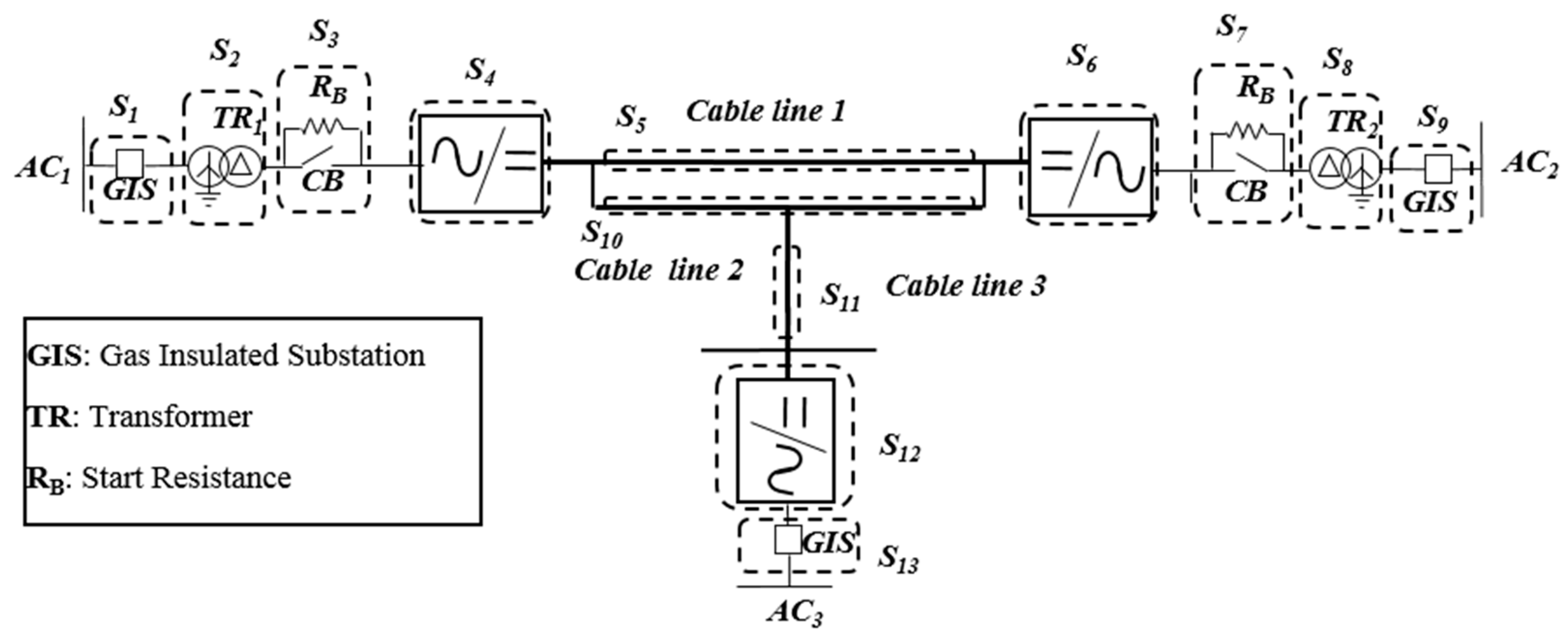
By considering a generic HVDC electrical scheme (see Figure 1), the overall availability As of the system can be expressed as the average proportion between the whole system up time and the sum of system up and down times [10,11].
To estimate As it is necessary to assess the availability Ai of every component or sub-system Sith which constitutes the HVDC link (see Figure 1) and to correctly combine them.
The starting point of this procedure is the knowledge of the failure rate λi [occurrence/year] and the repair rate µi [number of repairs/maintenance time] of each component. The more elementary way to assess Ai and As for a point-to point HVDC connection [10] is based on Equations (1) and (2):
where MTTFi = 1/λi is the Mean Time to Failure of the component (or sub-system) ith, MTTRi = 1/µi is its Mean Time to Repair and n is the number of components of the system.
Starting from these basic equations, several different and more detailed approaches have been developed in literature in order to estimate much more in depth the availability of complex configurations. In particular, it is possible to classify such methods on the basis of the procedures that they require to assess both the Ai and AS parameters and on the availability aspects that they are able to highlight.
3. Availability Assessment Methods for HVDC Systems
The most effective and practical methods that can be chosen to estimate the availability of HVDC links can be classified into two main categories:
- Analytical methods: Markov models, Multi State Matrix method and the Bayesian network-based approach;
- Simulative methods: sequential and non-sequential Monte Carlo approaches.
The application of analytical methods implies that the system availability is estimated as a unique average value. In this way, it is possible to know what the average outage time of the HVDC link is. The main advantage of this approach is that it is possible to compute AS with very short computation times, since the λi can be considered to be time-independent. This aspect makes the availability computation algorithms relatively simple. On the other hand, analytical methods do not give information about the probability distribution of the computed availability value and cannot consider the evolution of the system over the time. In contrast, simulative approaches give the user the knowledge of the probability distribution of AS, and are able to foresee the behavior, from an availability standpoint, of each component in a given working period. This makes it possible to describe the HVDC system in much more detail and implies considering the λi parameters as being time-dependent, entailing much more longer computation times. In the following, the particular characteristics of each method are presented and the main aspects that can be evaluated on the basis of the chosen approach are described.
3.1. Markov State Space Diagrams
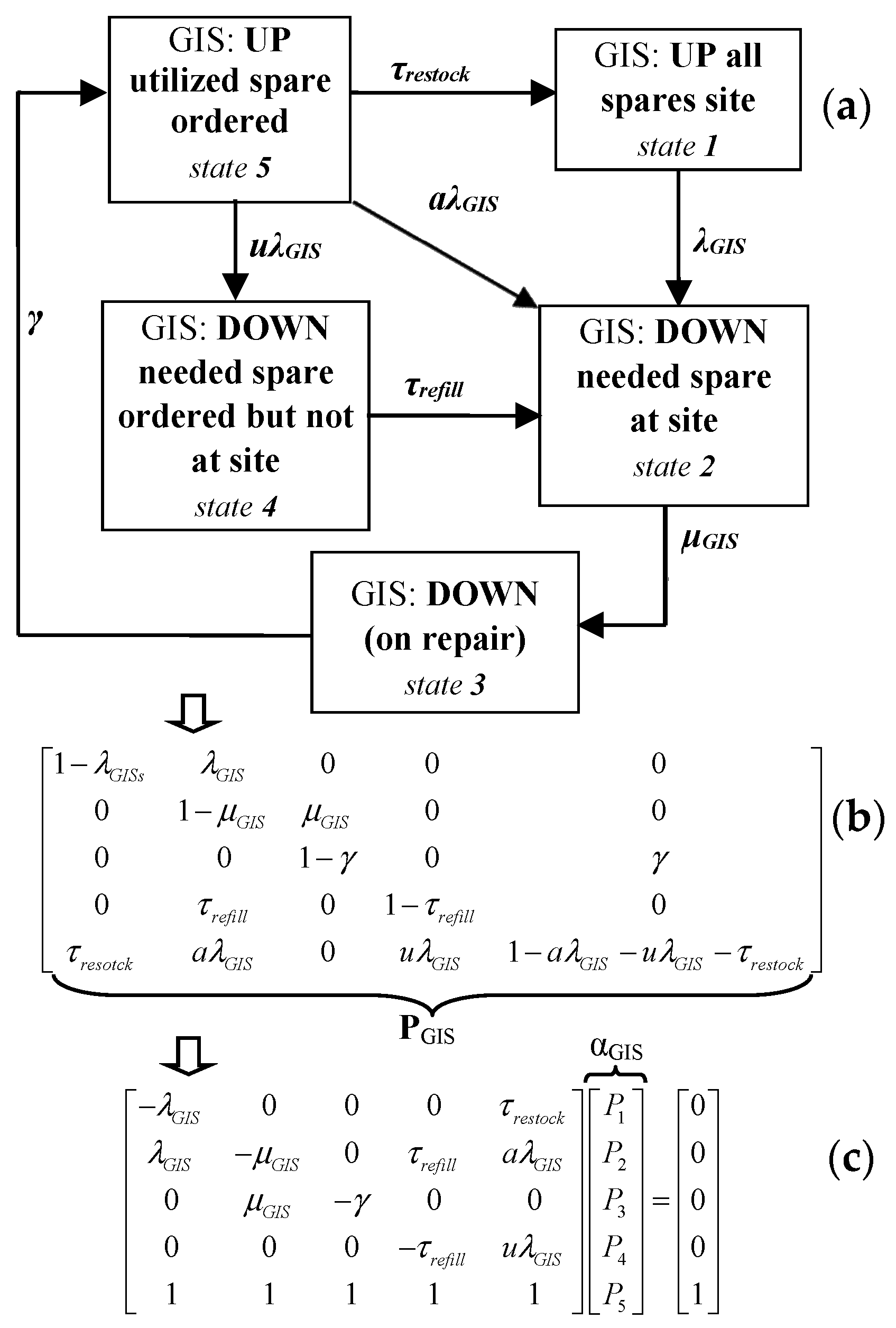
The possibility of taking into account the component spares of a HVDC link in the computation of AS can be very useful in order to optimize the spare management. This target can be achieved by exploiting the Markov state space diagrams [11,12,13]. By considering a single component of a HVDC point-to-point system, it is possible to analytically represent, in matrix form, the transitions of the component from one particular state to the other, with any spare management configuration. For example, for the GIS sub-systems of Figure 1, i.e., the sub-systems 1, 9 and 13, a possible Markov state space diagram is represented in Figure 2a [1], where:
- a is the probability that the needed parts for repair are available at site;
- u is the probability that the spare needed to repair the component is not available at site;
- τrestock is the local store replenish rate;
- τrefill is the lacking spare part’s refill rate;
- γ is the time rate for placing a component in service.
The up states of the sub-system represent possible operation configurations, whereas the down states represent the sub-system outage.
On the basis of the Markov theory, each state space diagram can be represented, in steady condition, in the matrix form [10]:
where α is called the limiting state probability vector. It consists of the unknown probabilities Px that the system is in a particular state x in one operating year, being:
with n_states number of possible states that the system ca assume (n_states = 5 in the example of Figure 2a). P is the stochastic transitional probability matrix, which depends on the paths from one state to the other in steady state condition, and it is inferable directly from the corresponding Markov state space diagram (see Figure 2b).
α·P = α
By taking into account (4), it is possible to solve the linear system represented by (3) by means of simple matrix algebra steps [10,11], obtaining the matrix representation of the GIS sub-system, which is shown in Figure 2c. Hence, the unknown probabilities Px (which are the elements of the vector α) can be obtained. The steady-state availability AGIS of the subsystem is the sum of the probabilities Px that the system is in an up state, x_up. For a generic sub-system i:
By applying the above described procedure to estimate the availability of the GIS sub-systems of Figure 1, which are supposed to be described by means of the state space diagram of Figure 2, and by assuming the values reported in Table 1, the GIS state space diagram represented in its matrix form in Figure 2c can be written as follows:
By solving this linear system, it is possible to obtain the unknown probabilities Px (with x=1,2,…,5) of the limiting state probability vector. The availability of the GIS sub-system can be computed by summing the probability P1 = 0.9995 and P5 = 0.0002 which are related to the up-states of the systems. Hence, the GIS availability is AGIS = P1 + P5 = 0.9995 + 0.0002 = 0.9997.
To compute the availability AS of the overall HVDC system, it is necessary to create a Markov state space diagram for each sub-system Si of the HVDC link (see in Figure 1), thereby to infer the availability Ai of each sub-system. Therefore, the overall system availability can be computed by means of (2). The main advantages of this approach lie in its simplicity and versatility. The computation burden is very low, from a fraction of a second to a few minutes, and it varies on the basis of both the link topology and the state-space diagram complexity. On the other hand, by applying the Markov models, AS is estimated only for the situation in which all the components of the HVDC system are functioning (up state), and, therefore, it does not correctly consider multi-terminal configurations which could be in a working state even if some sub-system is outage. Hence, the Markov approach is particularly useful for point-to-point HVDC connections. Theoretically, it is possible to extend the Markov approach to time dependent models [9,10], but this implies a considerable complication of the matrix modelling, therefore this solution is rarely applied.
3.2. Monte Carlo Approach
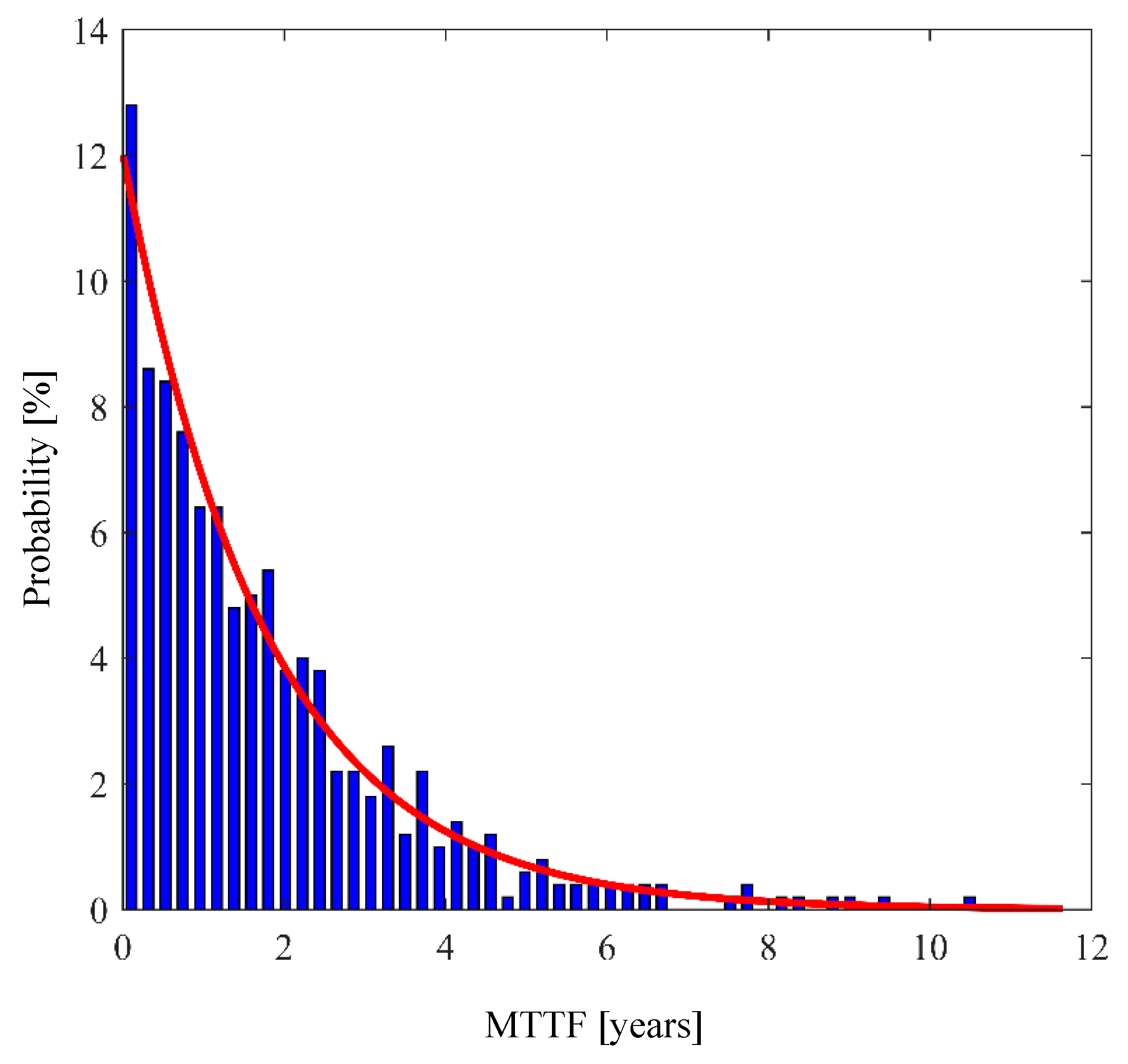
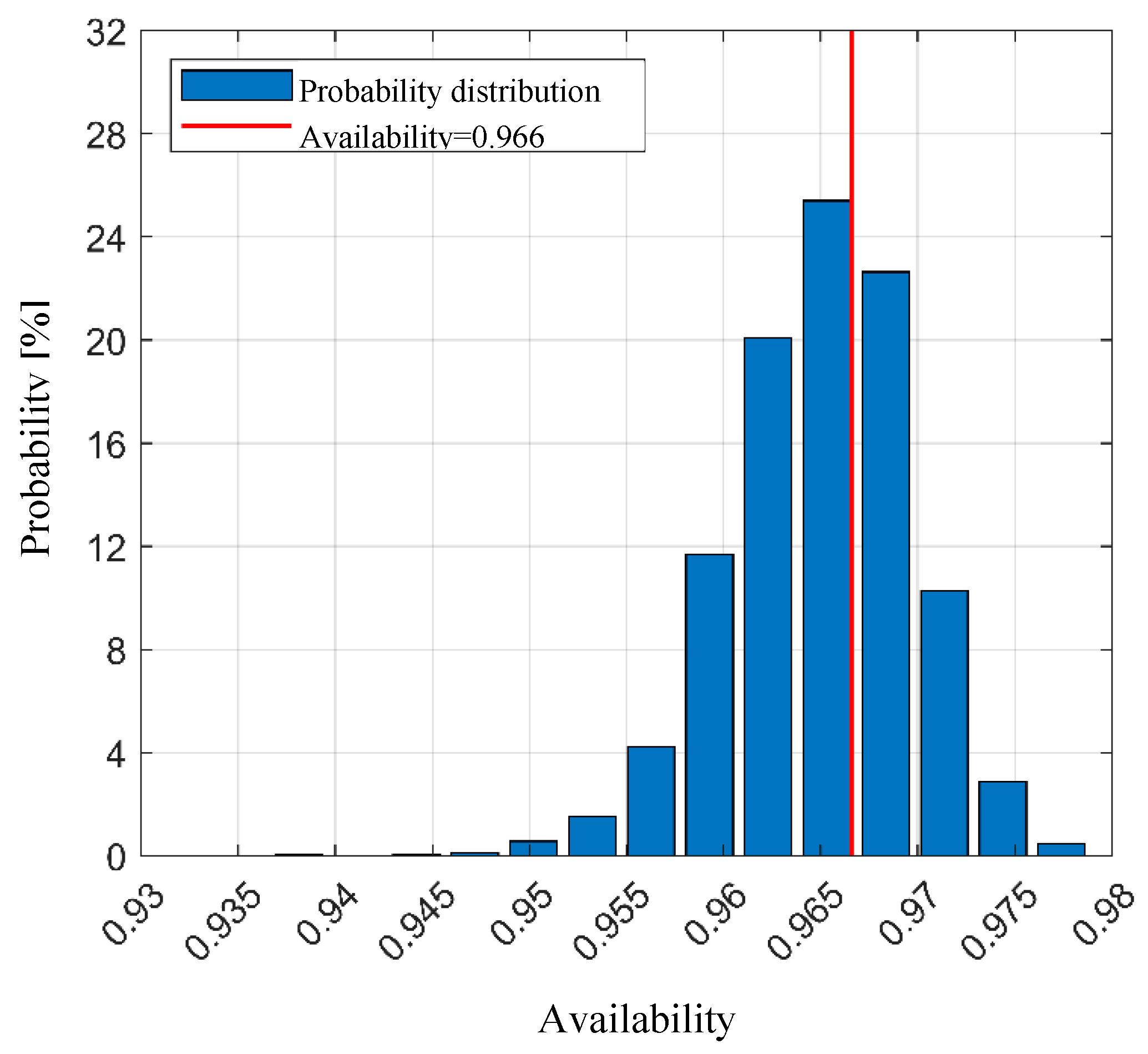
The opportunity to consider the MTTF data as time-dependent in the availability assessment of HVDC systems is closer to the real applications than considering an average unique MTTF value. In fact, if the MTTF varies as a function of time (see Figure 3), it is possible to obtain AS in the form of a probability distribution (see Figure 4). This implies the possibility of assessing AS in a specific time range. Such a target can only be achieved by applying methods exploiting the Monte Carlo approach [14,15,16,17], i.e., methods which are based on the generation of random number functions. The fundamental difference between this procedure and the analytical methods is that, starting from the λi and µi of the single components, the MTTF and MTTR are calculated as follows:
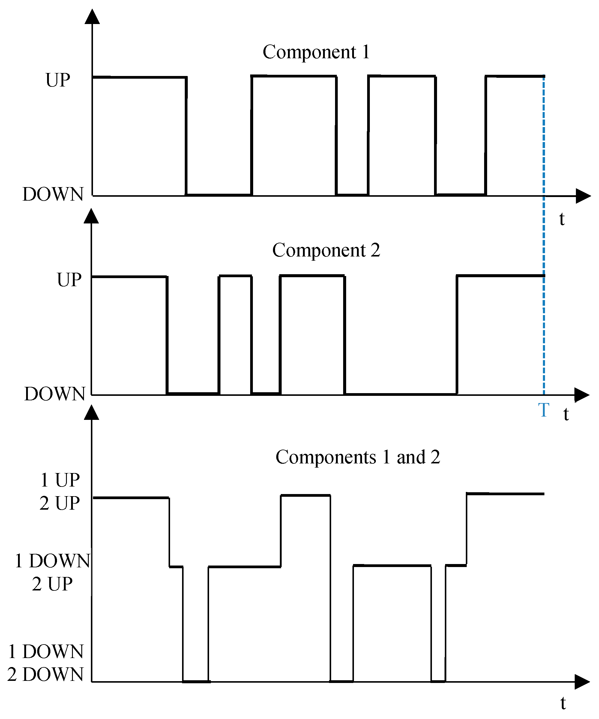
where Ni is a uniform distribution of random numbers, in a range between 0 and 1 for each component i. Thus, MTTF and MTTR distributions are combined with each other by applying the Monte Carlo algorithms [14,15] in order to create a diagram which shows the evolution of AS over the time. Figure 5 illustrates this concept for an ideal system composed of only two components. In other words, the availability of the system is computed by considering the working story of each component and by combining them together and sequentially.
This procedure is repeated a huge number of times by using a random number distribution in order to consider all the possible configuration of the system in the analyzed time range T. The higher the number of simulations, the higher the confidence of the results. If the procedure is correctly applied, the average value of AS should tend to the one obtained with analytical methods (red line in Figure 4).
The most interesting result from the application of the Monte Carlo approach to HVDC systems is the possibility of evaluating which are most probable system configurations in terms of the up or down state of each sub-system constituting the HVDC link within a chosen range of time.
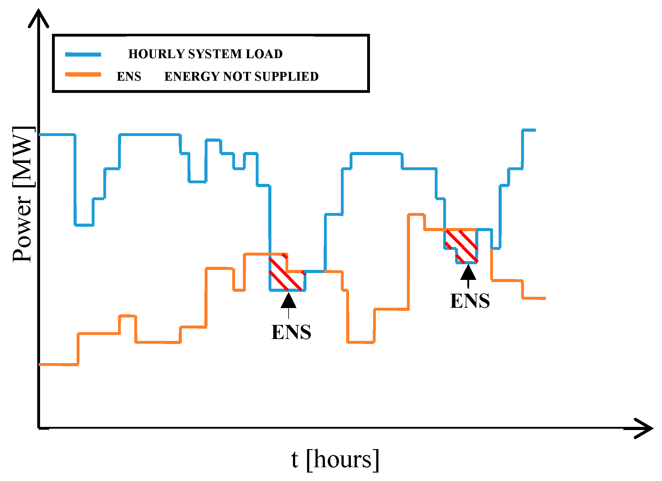
Each system configuration can be related to the corresponding transmittable power, and therefore, by knowing the electrical load profile of the system over the time, it is possible to estimate the transmissible power of HVDC interties on the basis of the electrical load variations (see Figure 6). This method can be effectively applied to multi-terminal HVDC schemes, but it may require great computation times, up to dozens of hours.
Alternatively, it is possible to apply the non-sequential Monte Carlo approach [16,17], which does not consider the evolution of each component over time, to HVDC systems.
The basic concept of this method is the generation of a random combination of n events, which determines n system configurations in terms of components which could be up or down for each event, on the basis of the λi values.
The system availability is computed as:
with n_up+n_down = n. Ti_up and Ti_down represent the time during which the system assumes an up or down configuration, respectively. This procedure is repeated for several simulations in order to obtain a probability distribution of the system availability. The main pros of the Monte Carlo non-sequential method are the very low computation burden—on the order of seconds or a few minutes based on the analyzed system complexity—and the possibility of applying it to multi-terminal HVDC configurations. On the other hand, it is not possible to consider the evolution of the system as a function of time and the working story of each component.
3.3. Multi-State Matrix Approach
Once the availability of each HVDC link sub-system has been computed (for example, by means of the Markov method or the Monte Carlo one), it is possible to estimate the average probability that the system is in a given configuration in terms of the up or down state of each component.
This target can be achieved by exploiting the matrix procedure developed in [18,19,20], where a system with several components, i = 1, …., n, each of which has several possible states, si, is described by means of a matrix Ci and a probability vector Pi. For an elementary system with a single component with two possible states, i.e., state 1 = up and state 2 = down, C1 and P1 are equal to:
The general iterative matrix procedures to obtain Ci and Pi for a generic system of n components are described in (9), where:
- Ci−1 is placed si times, so Ci has a total of column vectors, which are identified as the event vectors for the component events CE1(1), CE1(2), …, CE1(sn), CE2(1), CE2(2), …, CE2(sn);
- Pi(j) denotes the probability that the ith component takes the jth state, for i = 1, …, n, and j = 1, …, si.
An interesting application of this method is related to systems consisting of n components which can assume only two states [20]. In this case, the matrix representation of the system can be significantly simplified. In fact, the matrix Ci can be represented by means of a logical matrix Cl as a sequential descendant binary numeration from 2n − 1 to 0. For example, for a system with 3 components, the system matrix and the related probability vector are:
where the number of columns of the matrix Cl[3] are equal to the number of components c in the system, and the number of rows represents all the possible state combinations (23 for the case with 3 components) that the system can assume. As clearly explained in [20], with respect to the probability vector P[3] of the system, this can be obtained directly as follows: first, a matrix Cp[3] is formed by replacing the 1s and 0s in the matrix Cl with the corresponding probability Pi(1) and Pi(2), respectively:
The elements P of the probability vector P are obtained from Cp by multiplying the elements Pi(sj) by each other with respect to each row of Cl. In particular, the element Pi(1) can be seen as the availability Ai of the component i, whereas Pi(2) represents the component unavailability Ui.
Eventually, it is possible to estimate the availability of any chosen combination of component states, simply by applying the Boolean algebra between the columns c1, c2 and c3 of the matrix Cl in order to create the event vector Csys of the system. For example, a system with three components, all in up state, can be represented by means of (14):
i.e., by applying the AND operator (&) to the columns of Cl[3]. Finally, the probability P(Esys) that the chosen situation occurs can be obtained by (15):
In matrix form, (15) is equal to:
All the possible configurations of the system can be obtained by properly applying the logic operators AND, OR, NOR and EXOR to the columns of the matrix Cl. By relating the chosen configurations with the corresponding transmittable capacity, it is possible to estimate the average power capacity for each configuration or as a function of the parameters of interest.
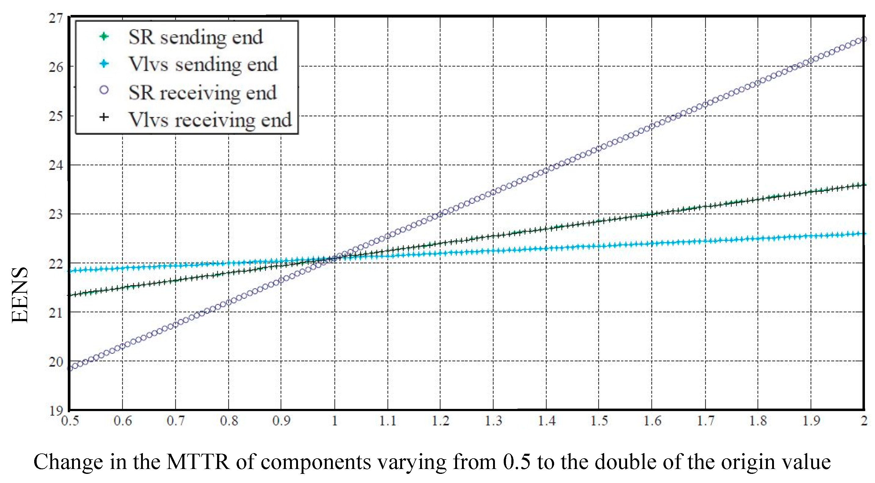
As an example, Figure 7 shows the Electrical Energy Not Supplied (EENS) for different MTTRs for a specific configuration of a HVDC system, computed by J.S.C. Jimenez et al. in [20].
Despite its simplicity, this method is very versatile, since it makes it possible to take into account the topology of the link and considering complex configurations of a HVDC system. Moreover, it can be combined with the Markov state space diagrams, and it is fully applicable to multi-terminal connections. The computation burden of this approach is very low, on the order of seconds or fractions of a second.
3.4. Bayesian Networks
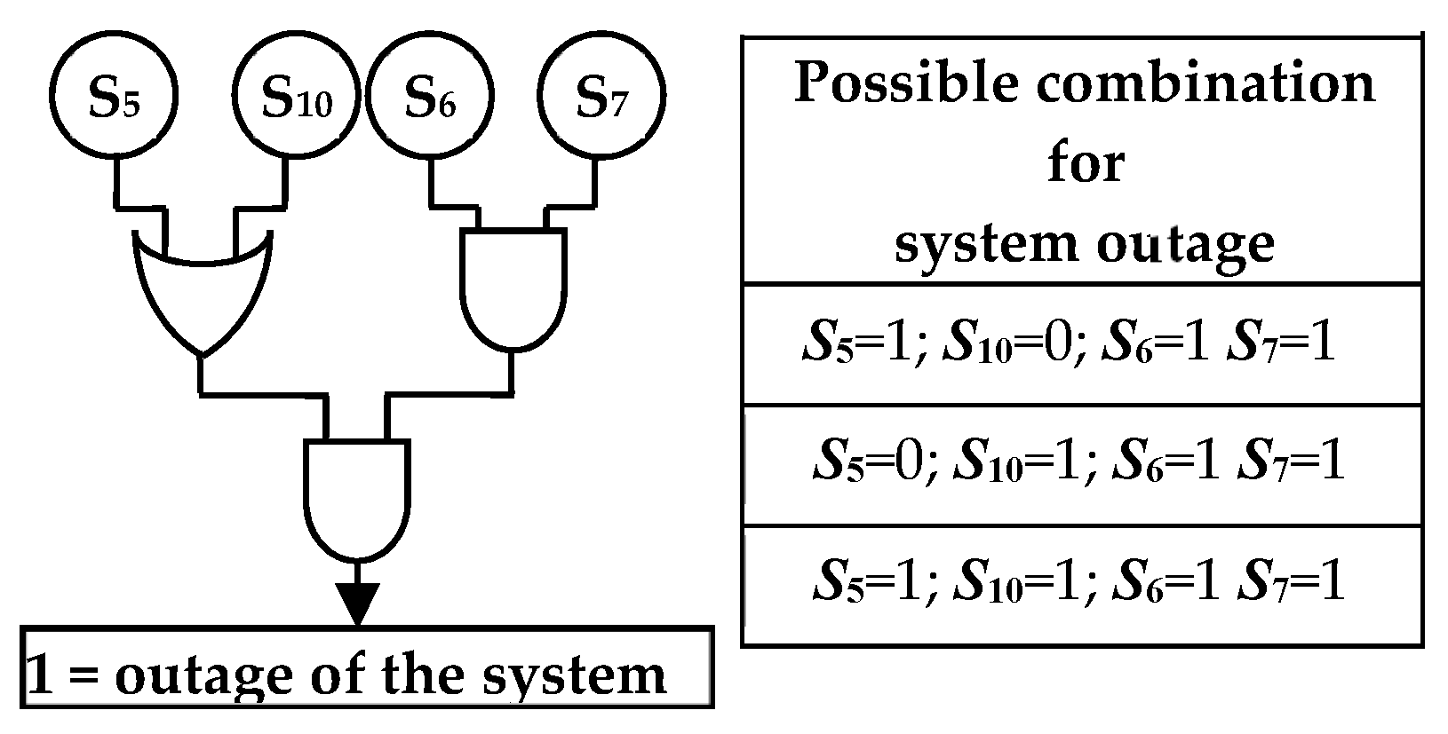
The application of the Bayes theorem in the availability assessment of a given HVDC link (point-to-point or multi-terminal) makes it possible to identify the most probable failure events which cause the outage of the system. This could be particularly useful in case of complex HVDC power transmission structures [21,22,23,24]. The connections between the components of the system are represented by means of logical gates: the AND gate is used for point-to-point connections, and the OR gate for the parallel ones. For example, by referring to Figure 1, the connections between the sub-systems S6, S11, S7, S8 can be represented as in Figure 8. The condition Si = 1 represents the outage of the subsystem Si.
By applying Boolean algebra between the logic gates, it is possible to identify the combinations which determine the outage of the considered system.
The overall Failure Probability (FP) is given by the combination of the failure probabilities P(Si)(Si=1) of each component:
where
FP = P(S5)·P(S7)·P(S6) + P(S10)·P(S7)·P(S6) + P(S5)·P(S10)·P(S6) + P(S7)
Hence, it is possible to estimate the conditioned probability P(FP|Si = 1) that the failure of the system is due to the failure of the component Si by applying the Bayes theorem:
The major advantages of this method are the possibility of applying it to multi-terminal connections and the low computation burden, which is on the order of seconds. Moreover, it is possible to consider how the electrical topology of the system affects its overall availability. Research to develop effective algorithms which are able to take into account the time dependence of λi when the Bayesian network approach is used is ongoing [25,26].
3.5. Summary of the Main Particularities of Each Computation Method
In Table 2, the main influence variables which can be considered with each of the described methods have been briefly summarized.
4. Overview of HVDC-VSC Modular Multilevel Converters
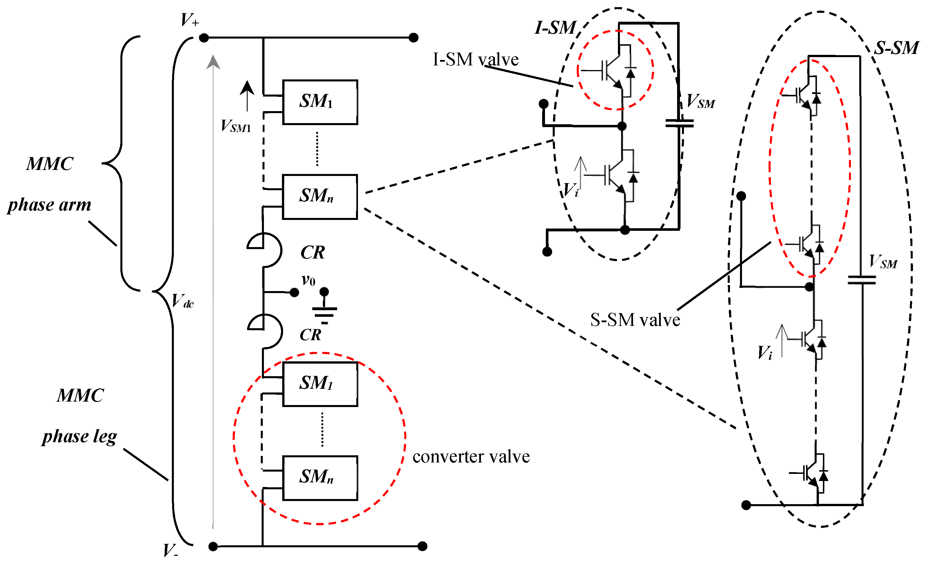
One specific feature of the most recent HVDC-VSC installations is the use of Modular Multilevel Converters (MMC), since converters with high numbers of voltage steps generate the requested output voltage waveform with a low harmonic content.
An MMC consists of three phase legs (pl), each of which is composed of an upper and a lower arm. Each arm includes a high number of sub-modules (SMs). The two most common SM architectures (see Figure 9) for HVDC-VSC applications consist of [27,28,29,30,31,32]:
- single-IGBT valves configuration, wire-bonded, base-insulated package, namely, I-SM;
- multiple IGBT valves configuration, namely, S-SM.
The SMs are connected in series with one converter reactor (CR), whose function is both to limit short-circuit currents through the valves in the event of a fault and to reduce the balancing currents between individual phases to very low values. Each sub-module basically contains:
- an IGBT-based half bridge (HB) converter (I-SM or S-SM type);
- a DC capacitor module for energy storage.
In both I-SM and S-SM configurations, each SM IGBT valve is able to work at the nominal SM voltage, though, usually, a safety voltage margin is foreseen. This is necessary for both voltage harmonic reduction and lifetime increase of single SMs (though, beyond voltage stress, other factors, like thermal stress and load profile, influence IGBTs and SM lifetime).
The de-rating factor η = Vi/Vw usually ranges in the interval (0.5 ÷ 0.7), where Vi is the actual operating voltage of the ith SM and Vw is its withstanding voltage [28].
In general, the nominal voltage of each SM is VSM = zηVw, where z is the minimal number of IGBTs in series inside the SM valve (z = 1 in the case of I-SM; z > 1 for S-SM).
Each arm consists of k = VDC/VSM SMs at least and it is able to generate k + 1 output voltage levels.
The arm voltage Varm is:
n − k redundant SMs, with n = k + m where m is the number of redundant SMs, ensure uninterrupted converter operation till failure of (n − k + 1) SMs.
Varm = Vpl/2 = kVSM = VDC
5. Conversion System Availability Estimation
As mentioned above, with the HVDC-VSC conversion system being a non-reparable item, its unavailability can be considered to be the down times during the scheduled maintenance period TM.
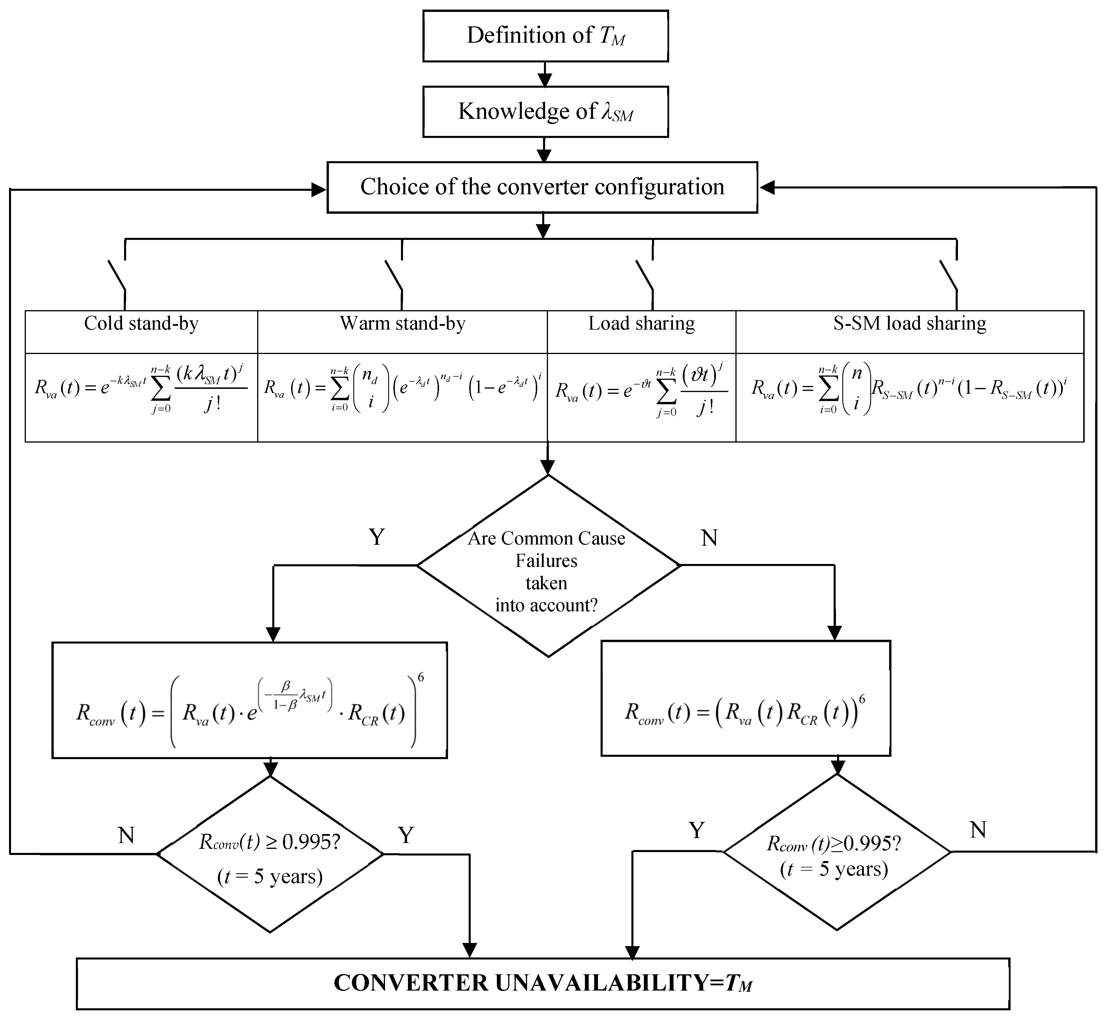
Hence, by estimating the reliability R(t) of the system, it is possible to identify the proper conversion system configuration that guarantees, from a statistical standpoint, uninterrupted working until the scheduled outage for maintenance, which is generally foreseen to be every one or two years. For example, a good approach could consist of the identification of a converter architecture for which the R(t) remains at a value ≥ 0.995 for at least five years from the start of operation.
This constraint implies an extremely high probability of uninterrupted operation of the MMC during the scheduled maintenance interval. This result can be obtained by means of the flow chart of Figure 10. Once the converter availability has been computed, all the approaches described in Section 3 and Section 4 can be applied by considering the conversion system as a reparable component whose availability is known.
In this section, the state of the art of the main formulations for assessing the reliability of the most widespread HVDC-VSC converter typologies are presented.
In general, the reliability function R(t) of one SM can be expressed as the product of the reliabilities of its components. For example, by considering only the reliability functions of the most vulnerable components like the IGBTs, the capacitor module and the gate unit, the SM reliability function can be expressed as [29,33,34]:
where:
, , and are the reliability functions of the IGBTs, of the capacitor module, and of the gate unit respectively. λIGBT, λCm and λgu are the corresponding failure rates.
The validity of the bathtub failure pattern for electronic components is recognized in the literature [24,28,29]. Hence, by assuming each module to be operating in the incidental failure period with all its components following exponential lifetime distributions, the reliability function RSM(t) of a SM may be written in exponential form as follows [10,11,28]:
where λSM is the failure rate of one SM.
The converter phase leg consists of one upper valve arm (at positive potential) and one lower valve arm (at negative potential) with a converter reactor connected in series to each valve arm (see Figure 9). Both valve arms contain n statistically identical independent distributed (i.i.d.) series connected SMs. k of them are sufficient to withstand the arm voltage, n-k are redundant. Such a system is called a “k-out-of-n redundant system”.
Hence, the reliability function Rva(t) of the converter valve-arm is the sum probability of having at the time t a number of surviving SMs greater than or equal to k. The Rva(t) formulation depends on the adopted redundancy strategy.
Once Rva(t) has been computed, it is possible to assess the reliability of the converter upper and lower arms, namely, Rua(t) and Rla(t), respectively, as follows:
where RCR is the reliability of the converter reactor. Since one phase leg works only if both its upper and lower arms work, the phase leg reliability Rpl(t) is:
The whole converter only works if all three phases simultaneously operate. Its reliability function RConv(t) is therefore:
In the following, the analytical procedures to estimate Rva(t) on the basis of the chosen redundancy strategy are summarized, whereas the converter availability can be computed by following the flow-chart in Figure 10.
5.1. Converter Reliability Computation in Passive Redundant Configuration
The passive redundant mode is characterized by the presence of idle or partially loaded standby redundant SMs. This redundancy configuration comprises the cold stand-by mode and the warm stand-by one. In the cold stand-by mode, (n − k) SMs are assumed to initially be idle with zero failure rate (no SM failure possible in standby mode). At any time, k identical SMs work in series with individual failure rate λSM: the series working failure rate is equal to the sum of components failure rates. Upon failure of one working SM, it is disconnected and bypassed by a high-speed mechanical switch, while one redundant unit is switched into operation by a control system to replace the faulted unit. The mean voltage applied to each working SM defined by the arm output voltage is constant, not depending on the number of surviving redundant SMs. The bypass of the faulted item and the passage to full operation of the standby SM actually need time: a transient interval, including SM charging, affects converter operation. The risk of switching failures should be taken into account. In this case, the valve arm series subsystem shows a failure rate k⸱λSM, which follows an exponential distribution. This is due to the memory-less property of the exponential distribution: each one of the k SMs included in a new subseries is assumed to be as good as new. As soon as the kth redundant SM fails, the valve arm and the whole converter fail. The converter valve arm reliability for the case of k out of n cold standby redundancy can be estimated by means of (25) [35]:
In reality, redundant standby SMs are initially energized (i.e., the SM capacitor is charged) so that redundant SMs are considered to be in a dormant state. They are often cyclically switched by a control function from standby to active operation to the purpose of uniform exploitation of all SMs in the arm. Standby SMs may fail in dormant state, whereas active SMs may fail in operation. All identical SMs show exponential distributed lifetimes with parameter λd in the dormant state and λo in the active state, respectively (normally, λd << λo). By hypothesizing perfect sensing and switching and by excluding the occurrence of simultaneous SMs failures, the closed form Equation (26) for the reliability estimation of a warm standby redundant system was obtained by She et al. in [36]. When λd = 0, the equation gives the reliability of the k out of n cold standby redundant valve-arm system.
5.2. Converter Reliability Computation in Active Redundant Configuration
In the active redundant mode, all the redundant and non-redundant SMs in the converter arm work. This redundancy configuration comprises the load sharing mode and the conventional one. In the farmer, all n SMs equally share the total arm voltage. In this case, all the n = k + m SMs resist a voltage at any moment; the instantaneous voltage blocked by each SM is initially lower than its nominal voltage, whereas the mean SM switching frequency is higher. The voltage applied to each SM increases upon failure of one SM in the arm; consequently, the SM failure rate λSM increases in direct proportion to the increasing voltage applied.
Upon failure of the ith SM, the individual SM failure rate λi_SM of each of the n-i surviving SMs is:
λ0_SM ≤ …. λi_SM ≤ …. ≤ λn−k_SM with 0 ≤ i ≤ n − k.
The converter works until only k SMs survive, resisting the nominal arm voltage.
In contrast, in the conventional mode the number of voltage levels k + 1 is constant and an optimization algorithm chooses time k SMs at any to be switched on from among all n SMs. The reference voltage of each SM remains constant upon failure of one SM at its initial nominal value. As several SMs larger than the minimum are needed for the converter operation is available, the mean SM switching frequency is lower and at any time several SMs bear zero voltage. With a greater number of working SMs per arm, the control and voltage-balancing algorithms have a larger set of SMs from which selecting the unit to connect or bypass in the next switching instant. The percent switching frequency reduction per SM, proportional to the number of active redundant SMs, is equal to (k/(k + m))⋅100. It is worth noting that the lower mean voltage stress imposed to SMs in load sharing mode versus conventional mode qualitatively implies a reduced failure rate, as explained in [38]; therefore, this configuration is the most widely used.
The formulation which is usually applied to assess converter valve arm reliability in the load sharing mode [35] is the following:
where:
ϑ is constant for each i = 1,2, …, n − k + 1.
5.3. S-SM MMC Reliability Calculation
One S-SM consists of two multiple-IGBT valves and one storage capacitor in logical series. The whole S-SM fails if any of the component subassemblies fails. IGBTs in the same SM must switch simultaneously. An effective way to extend S-SM lifetime is to include redundant IGBTs in each S-SM valve. Given that z is the minimum number of IGBTs able to withstand the S-SM blocking voltage, the addition of a suitable number m = s − z of active redundant IGBTs, (with s total number of IGBTs per S-SM) allows fault-tolerant operation of the S-SM upon the failure of individual redundant IGBTs. At the beginning, all IGBTs are good, and their initial constant failure rate is λ0_S-SM. When the ith IGBT fails, the s-i surviving units continue to operate, sharing the nominal S-SM voltage in equal proportion, and thereby withstanding an increased voltage. In other words, a S-SM unit is always managed in an active redundant configuration, in load sharing mode. Hence, in order to estimate the reliability RS-SM of one S-SM valve, (28) can be applied to the single S-SM as follows:
with ϑS−SM = ϑi_S−SM = (s − i)·λi−1_S-SM.
ϑS-SM is constant for each i = 1,2, …, s − z + 1.
Since the adopted redundancy strategy for a S-SM converter is usually the warm stand-by one, the reliability of a S-SM converter valve arm can be estimated by means of (30):
It is worth noting that (30) is formally equal to (27).
5.4. Converter Common Cause Failure
In the above-described formulations, all the SMs were assumed to be identical and independent from one another. Each one fails independently from all others, i.e., the failure of any SM does not affect the state of the other ones in the arm. The independent failure assumption may not be applicable in practice: a single or common cause can affect more than one component and cause several components to fail simultaneously. Common cause failures (CCFs) may limit the reliability improvements gained by adding redundancies to the system; thereby, they are relevant for converters, whose fault-tolerant behaviour is reliant on the presence of redundant SMs. Hence, the analytical equations for inferring MMC converter reliability should be modified to evaluate the impact of CCF. The correct quantitative evaluation of CCFs would require a large set of parameters (the failure probabilities of specific groups of units), which increases quickly with the number of redundant units. Parametric models requiring all this information, which is not supplied by statistical records, are impossible to implement. The Basic Parametric Model (BPM) [38] introduces simplifying assumptions (above all, the symmetry assumption) that significantly reduce the total number of required parameters.
These constraints have imposed the β-factor model approach, which imposes the least stringent requirements. Despite its simplifications, the BPM is also not a feasible method in the majority of practical situations, being characterized by severe lack of operational statistics.
The β-factor model is the most commonly used in reliability analysis [10,11,39]; it is easy to handle and provides reasonably correct, conservative (for high levels of redundancy) results. It needs only two parameters, as only two failure types are modelled: the individual unit independent failure rate (λSM) and the failure rate λcc related to the simultaneous failure of all units as consequence of a common cause.
All common-cause failures result in the failure of all the redundant SMs. This simplification permits to introduce only one additional parameter in the independent failure model.
The total failure rate λT is defined as λT = λSM+λcc.
Hence, by defining the parameter β = λcc/λT, the converter valve arm reliability in presence of CCFs is:
5.5. Converter Reliability as a Function of the Redundancy Configuration: Calculation Examples
To better understand how the above-mentioned formulations work, in this section, the reliability of a hypothetic ±320 kV HVDC-VSC converter, composed of 4.5 kV SMs, has been calculated as a function of:
- SMs typology: either I-SMs composed of two 4.5 kV IGBTs or S-SMs composed of s 4.5 kV IGBTs in series per valve;
- Redundancy strategy: cold standby, warm standby and active load sharing for I-SM MMC; active load sharing for S-SM MMC;
- Minimum SM number (k) per valve arm, resulting from the nominal arm voltage and the applied de-rating factor;
- Percentage r of redundant SMs.
The preliminary step of this analysis is to know the converter SM failure rates λSM. These data were inferred from [40,41] based on the SM typology, i.e., stack pack or high pack SM. The second step is to choose the scheduled maintenance period TM of the converter. Hence, the flow chart in Figure 10 is applied on the basis of the converter typologies and of the redundancy configurations.
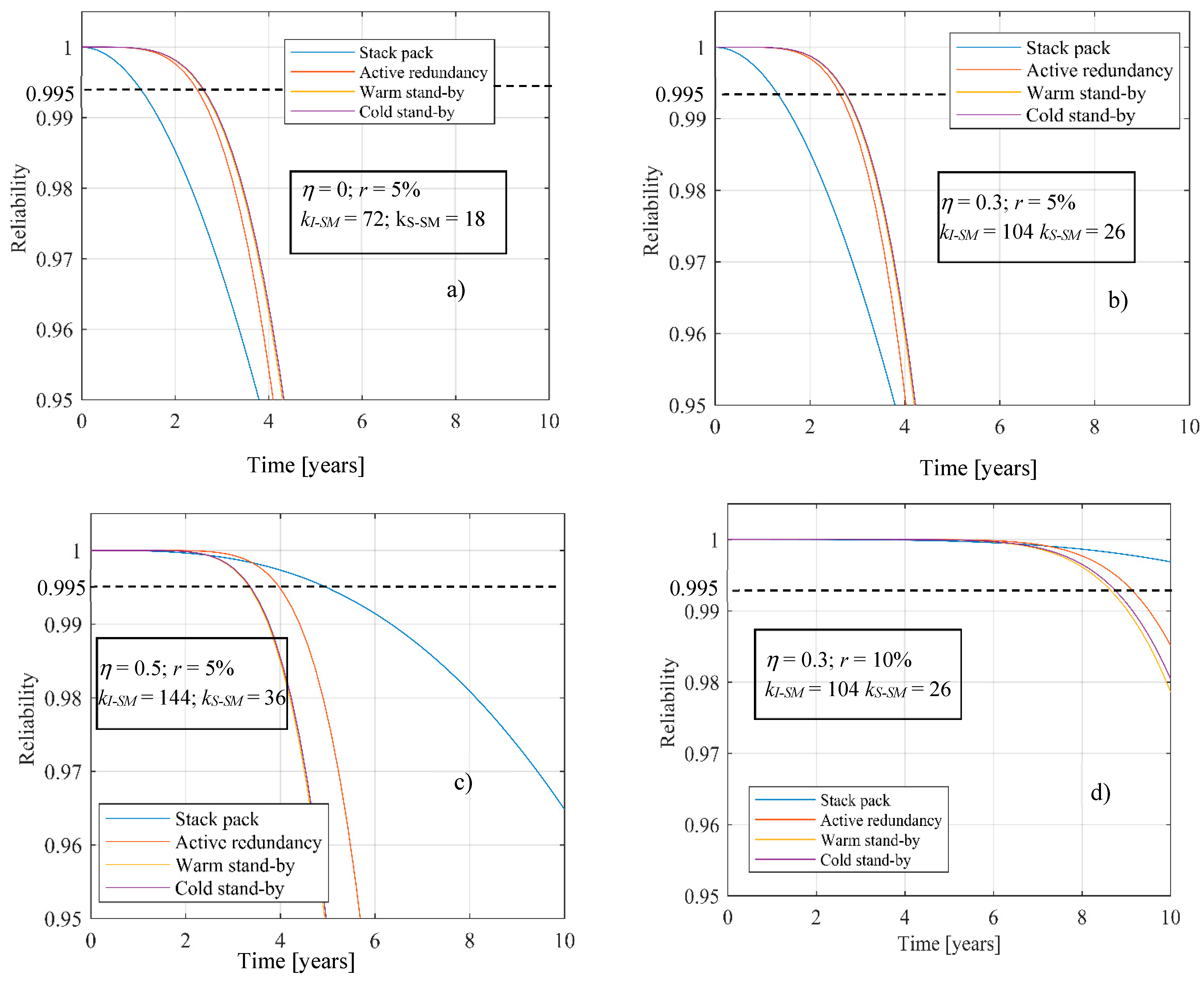
The purpose of this reliability analysis is to identify, by means of the described analytical formulae, the converter redundancy architectures that have R(t) ≥ 0.995 at least for five years from the start of the operation. This constraint implies an extremely high probability of uninterrupted operation of the MMC during the scheduled maintenance interval (two years). The number of IGBTs is the same for each analyzed converter configuration, with λSM = 0.004 and λd = 0.001 [40,41,42] (for the warm standby configuration).
As is possible to see in Figure 11, the constraint R(t) ≥ 0.995 for the first five years is verified for the curves Figure 11c,d. In fact, the parameters kI-SM, kS-SM, η and the percentage redundancy r of Figure 11c are consistent with the ones typically applied to real converter installations.
It is interesting that the reliability of the S-SM configuration increases more than the other ones as the number of redundant SMs is increased.
The reason S-SM configuration shows a lower reliability in Figure 11a can be attributed to the fact that redundant SMs are present only at the arm level and not at the valve one.
This choice was adopted to perform the comparisons of Figure 11 maintaining a constant IGBT number, even if commercial S-SM converters typically use redundancy at the valve level, with the consequent reliability grow.
The difference between the reliability of the active redundant mode and the warm standby one is negligible, and it becomes apparent above 10% of SMs redundancy (see Figure 11d).
Figure 11a shows the converter R(t) behaviour with r = 5%, kI-SM = 72, kS-SM = 18 and η = 0, for the different redundancy strategies. Obviously, this is only a theoretical configuration, and not to be used in practice, but it is useful to understand the influence of the redundancy and of the de-rating choices on the R(t) behaviour.
6. Conclusions
In this paper, an overview of the tools developed in the scientific literature for estimating the overall availability of HVDC-VSC systems is presented.
The paper highlights that, by exploiting analytical approaches, it is possible to consider specific variables that affect the average overall availability of a HVDC system. In particular, the Markov state space diagrams are useful for taking the spare management into account, the Bayesian network approach allows considering the failure conditioned probabilities of the system, and the multi-state matrix method is able to estimate the transmittable power capacity based on the system operating configuration.
At present, no analytical modelling is able to consider the time dependence of the availability and reliability functions. On the other hand, analytical approaches present a very low computation burden and are very versatile and adaptable to the specific needs of the users. For example, for HVDC monopolar systems typically used for land installations, the Markov state space approach is very effective, since it allows describing the HVDC link with a great detail. For bipolar or multi-terminal systems, the best option may be the combination of Markov theory with the multi-state matrix method.
Differently, simulative methods are able to represent the availability and reliability evolution of a HVDC system over the time, by taking into account all the possible operating states that the system can assume. By contrast, the computation burden of this approach is considerable, and it does not allow considering some variables which affect the overall availability of the system, such as the spare management or the failure conditioned probability of the system.
Moreover, the paper expounds a procedural approach to estimate the reliability and availability of HVDC-VSC MMC conversion systems, by exploiting the most effective analytical procedures presented in literature on the basis of the converter technologies and the chosen redundancy strategies.
Hence, what emerges from the paper is that to perform an availability analysis of HVDC-VSC links as accurately as possible, it is necessary to synergistically apply and combine the output data of different approaches.
It is worth noting that, in order to thoroughly understand all the potentialities that each availability estimation approach offers, it would be interesting to apply the described methods to an existing HVDC link and to compare the results provided by each one. For this purpose, it is important to collect the failure rates and the time to repair data of all the sub-systems of the link. The authors are working on reaching this target for a real HVDC installation.
Author Contributions
S.D.S. wrote and reviewed the paper, conceived the paper idea and performed the analyses of the availability estimation tools. A.C. has contributed to the work of analysis of the availability estimation tools and to the paper revision. R.B. acquired the founding resources, reviewed and approved the final paper and supervised the entire work.
Funding
This research received no external funding.
Conflicts of Interest
The authors declare no conflict of interest.
References
- Dambone Sessa, S.; Chiarelli, A.; L’abbate, A.; Benato, R. Availability Assessment Methods for HVDC Systems: A Review. In Proceedings of the 2019 AEIT HVDC International Conference (AEIT HVDC), Florence, Italy, 9–10 May 2019. [Google Scholar]
- Silva, B.; Moreira, C.L.; Seca, L.; Phulpin, Y.; Lopes, J.P. Provision of Inertial and Primary Frequency Control Services Using Offshore Multiterminal HVDC Networks. IEEE Trans. Sustain. Energy 2012, 3, 800–808. [Google Scholar] [CrossRef]
- Rink, Y.; Held, L.; Wenig, S.; Suriyah, M.; Leibfried, T. Utilization of MMC-HVDC for Primary and Secondary Control in Hybrid ACDC Power Systems. In Proceedings of the 53rd International Universities Power Engineering Conference, Glasgow, UK, 4–7 September 2018. [Google Scholar]
- Pierria, E.; Bindera, O.; Hemdanab, N.G.A.; Kurrata, M. Challenges and opportunities for a European HVDC grid. Renew. Sustain. Energy Rev. 2017, 70, 427–456. [Google Scholar] [CrossRef]
- Haileselassie, T.M.; Uhlen, K. Primary frequency control of remote grids connected by multi-terminal HVDC. In Proceedings of the IEEE PES General Meeting, Providence, RI, USA, 25–29 July 2010. [Google Scholar]
- Barnes, M.; van Hertem, D.; Teeuwsen, S.P.; Callavik, M. HVDC Systems in Smart Grids. Proc. IEEE 2017, 105, 2082–2098. [Google Scholar] [CrossRef]
- Benato, R.; Dambone Sessa, S.; de Zan, R.; Pazienza, M.; Rebolini, M. Italy-France Piemonte-Savoia HVDC Interconnection: An example of synergy between electric energy transmission and motorway transport. Proc. CIGRÉ 2018, 11, 2712–2720. [Google Scholar]
- Benato, R.; Forzan, M.; Marelli, M.; Orini, A.; Zaccone, E. Harmonic behaviour of HVDC cables. Electr. Power Syst. Res. 2012, 89, 215–222. [Google Scholar] [CrossRef]
- Mazzanti, G.; Marzinotto, M. Extruded Cables for High-Voltagedirect-Current Transmission; JohnWiley & Sons: Hoboken, NJ, USA, 2013. [Google Scholar]
- Billinton, R.; Allan, R.N. Reliability Evaluation of Engineering Systems, 2nd ed.; Springer Science + Business Media: New York, NY, USA, 1992. [Google Scholar]
- Rausand, M.; Hoyland, A. System Reliability Theory: Models, Statistical Methods and Applications, 2nd ed.; John Wiley & Sons: Hoboken, NJ, USA, 2004. [Google Scholar]
- Benato, R.; Chiarelli, A.; Sessa, S.D.; Napolitano, D. Overall Availability Assessment of HVDC VSC XLPE Cable Symmetrical Monopolar Configuration. In Proceedings of the 2017 AEIT International Annual Conference, Cagliari, Italy, 20–22 September 2017. [Google Scholar]
- Benato, R.; Chiarelli, A.; Sessa, S.D.; Napolitano, D.; Rinzo, G. Valutazione della disponibilità di sistemi HVDC VSC monopolari simmetrici in cavo. L’Energia Elettrica 2018, 95, 3–10. [Google Scholar]
- Billinton, R.; Li, W. Reliability Assessment of Electric Power Systems Using Monte Carlo Methods; Springer: New York, NY, USA, 1994. [Google Scholar]
- Rubisten, R.; Kroese, D. Simulation and the Monte Carlo Method; John Wiley & Sons: Hoboken, NJ, USA, 2017. [Google Scholar]
- Billinton, R.; Sankarakrishnan, A. A comparison of Montecarlo Simulation techniques for composite power system reliability assessment. In Proceedings of the IEEE WESCANEX 95 Conference on Communications, Power, and Computing, Winnipeg, Manitoba, 15–16 May 1995. [Google Scholar]
- Billinton, R.; Sankarakrishnan, A. Adequacy Assessment Of Composite Power Systems With Hvdc Links Using Monte Carlo Simulation. IEEE Trans.Power Syst. 1994, 9, 1626–1633. [Google Scholar] [CrossRef]
- Song, J.; Kang, W.H. System reliability and sensitivity under statistical dependence by matrix-based system reliability method. Struct. Saf. 2009, 31, 148–156. [Google Scholar] [CrossRef]
- Kang, W.H.; Song, J.; Gardoni, P. Matrix-based system reliability method and applications to bridge networks. Reliab. Eng. Syst. Saf. 2008, 93, 1584–1593. [Google Scholar] [CrossRef]
- Contreras-Jiménez, J.S.; Rivas-Dávalos, F.; Song, J.; Guardado, J.L. Multi-state system reliability analysis of HVDC transmission systems using matrix-based system reliability method. Int. J. Electr. Power Energy Syst. 2018, 100, 265–278. [Google Scholar] [CrossRef]
- Bobbio, A.; Portinale, L.; Minichino, M.; Ciancamerla, E. Improving the analysis of dependable systems by mapping fault trees into Bayesian networks. Reliab. Eng. Syst. Saf. 2001, 71, 249–260. [Google Scholar] [CrossRef]
- Torres-Toledano, J.G.; Sucar, L.E. Succar: Bayesian Networks For Reliability Analysis Of Complex Systems. Lect. Notes Comput. Sci. 1998, 1484, 195–206. [Google Scholar]
- Laggoune, R.; Hassene, A.; Chateauneuf, A. Bayesian networks for the evaluation of complex system’s availability. In Proceedings of the 8th International Workshop on Verification and Evaluation of Computer and Communication Systems, Bejaïa, Algeria, 29–30 September 2014. [Google Scholar]
- Tourgoutian, B.; Yanushkevich, A.; Marshall, R. Reliability and availability model of offshore and onshore VSC-HVDC transmission systems. In Proceedings of the 11th IET International Conference on AC and DC Power Transmission, Birmingham, UK, 10–12 February 2015. [Google Scholar]
- Nodelman, U.; Shelton, C.R.; Koller, D. Continuous time bayesian networks. In Proceedings of the Eighteenth Conference on Uncertainty in Artificial Intelligence, Edmonton, AB, Canada, 1–4 August 2002; pp. 378–387. [Google Scholar]
- Boudali, H.; Dugan, J.B. A discrete-time Bayesian network reliability modeling and analysis framework. Reliab. Eng. Syst. Saf. 2005, 87, 337–349. [Google Scholar] [CrossRef]
- Marquardt, R.; Lesnicar, A. New Concept for High Voltage-Modular Multilevel Converter. In Proceedings of the PESC 2004 Conference, Aachen, Germany, 20–25 June 2004. [Google Scholar]
- Guo, J.; Liang, J.; Zhang, X.; Judge, P.D.; Wang, X.; Green, T.C. Reliability Analysis of MMCs Considering Sub-module Designs with Individual or Series. IEEE Trans. Power Deliv. 2016, 32, 666–677. [Google Scholar] [CrossRef]
- Jacobson, B.; Karlsson, P.; Asplund, G.; Harnefors, L.; Jonsson, T. VSC-HVDC transmission with cascaded two-level converters. Proc. Cigré 2010, B4–B110. Available online: https://ecigre.org/search_results.asp?page=1&nb_limit=9&keywords_title_ref=492&publication_type=1 (accessed on 15 June 2019).
- Westermann, D.; Van Hertem, D.; Real, G.; Rauhala, T.; Meisingset, M.; Kurrat, M.; Deppe, B.; Atmuri, R.; Küster, A.; Soerangr, D.; et al. Cigré Technical Brochure # 492. Voltage Source Converter (VSC) HVDC for Power Transmission–Economic Aspects and Comparison with other AC and DC Technologies. 2012. Available online: https://www.semanticscholar.org/paper/Voltage-Source-Converter-(VSC)-HVDC-for-Power-and-Westermann-Hertem/45b28196660499af79bf0fd27ca95f845e9fb6ff (accessed on 15 June 2019).
- Bauer, J.G.; Wissen, M.; Gutt, T.; Biermann, J.; Schäffer, C.; Schmidt, G.; Pfirsch, F. New 4.5 kV IGBT and diode chip set for HVDC Transmission Applications. In Proceedings of the PCIM Europe, Nuremberg, Germany, 20–22 May 2014. [Google Scholar]
- Kaufmann, S.; Lang, T.; Chokhawala, R. Innovative Press Pack Modules for High Power IGBTs. In Proceedings of the 13th International Symposium on Power Semiconductor Devices & ICs, Osaka, Japan, 7 June 2001. [Google Scholar]
- Xie, M.; Lai, C.D. Reliability analysis using an additive Weibull model with bathtub-shaped failure rate function. Reliab. Eng. Syst. Saf. 1996, 52, 87–93. [Google Scholar] [CrossRef]
- Wang, B.; Wang, X.; Bie, Z.; Judge, P.D.; Wang, X.; Green, T.C. Reliability Model of MMC Considering Periodic Preventive Maintenance. IEEE Trans. Power Deliv. 2017, 32, 1535–1544. [Google Scholar] [CrossRef]
- Kuo, W.; Prasad, R.; Tillman, F.A.; Mwang, C.L. Optima Reliability Design: Fundamentals and Applicatios; John Wiley and Sons: Hoboken, NJ, USA, 2003. [Google Scholar]
- She, M.; Pecht, G. Reliability of a out of warm-standby sstem. IEEE Trans. Reliab. 1992, 41, 72–77. [Google Scholar] [CrossRef]
- Amari, S.V.; Pham, H.; Misra, R.B. Reliability Characteritics of k-out-of-n Warm Standby. IEEE Trans. Reliab. 2012, 61, 1007–1018. [Google Scholar] [CrossRef]
- Guo, J.; Wang, X.; Liang, J.; Pang, H.; Goncalves, G. Reliabiliy Modelling and Evaluation of MMCs Under different Redundancy Schemes. IEEE Trans. Power Deliv. 2017, 33, 2087–2096. [Google Scholar] [CrossRef]
- Kalaiselvan, C.; Rao, L.B. Comparison of reliability techniques of parametric and non-parametric method. Eng. Sci. Technol. Int. J. 2016, 19, 691–699. [Google Scholar] [CrossRef] [Green Version]
- Beddard, A.; Barnes, M. VSC-HVDC Availability Analysis; The University of Manchester: Manchester, UK, 2011. [Google Scholar]
- Cigre Technical Brochures 510, 511, 513: Final Report of 2004-2007 International Enquiry on Reliability of High Voltage Equipment. 2007. Available online: https://e-cigre.org/publication/512-final-report-of-the-2004---2007-international-enquiry-on-reliability-of-high-voltage-equipment---part-4-instrument-transformers (accessed on 15 June 2019).
- Benato, R.; Chiarelli, A.; Dambone Sessa, S.; de Zan, R.; Pazienza, M.; Rebolini, M. La Piemonte–Savoia: la nuova interconnessione tra Italia e Francia con tecnologia HVDC-VSC. L’Energia Elettrica 2018, 95, 29–38. [Google Scholar]
Figure 1.
Electrical scheme of a HVDC multi-terminal connection divided in sub-systems.

Figure 2.
Representation of the GIS sub-system by means of the Markov theory: (a) Markov state space diagram of the GIS subsystem; (b) stochastic transitional probability matrix; (c) matrix representation of the GIS state space diagram.
Figure 2.
Representation of the GIS sub-system by means of the Markov theory: (a) Markov state space diagram of the GIS subsystem; (b) stochastic transitional probability matrix; (c) matrix representation of the GIS state space diagram.

Figure 3.
MTTF in the form of probability distribution for the application of the Monte Carlo approach.
Figure 3.
MTTF in the form of probability distribution for the application of the Monte Carlo approach.

Figure 4.
Typical output of the Monte Carlo approach: the probability distribution of the availability of a given system.
Figure 4.
Typical output of the Monte Carlo approach: the probability distribution of the availability of a given system.

Figure 5.
Graphical representation of the working history of a simple system consisting of two components.
Figure 5.
Graphical representation of the working history of a simple system consisting of two components.

Figure 6.
Energy not supplied for a HVDC system as a function of the electrical load variation.

Figure 7.
Electrical Energy Not Supplied (EENS) for different MTTRs computed by means of the multi-state matrix approach computed by J.S.C. Jimenez et al. in [20].
Figure 7.
Electrical Energy Not Supplied (EENS) for different MTTRs computed by means of the multi-state matrix approach computed by J.S.C. Jimenez et al. in [20].


Figure 9.
I-SM and S-SM MMC configurations.

Figure 10.
Procedure to determine the conversion system availability on the basis of the chosen redundant configuration.
Figure 10.
Procedure to determine the conversion system availability on the basis of the chosen redundant configuration.

Figure 11.
R(t) of the converter as a function of r, kI-SM, kS-SM, and η: (a) r = 5%, kI-SM = 72, kS-SM = 18 and η = 0; (b) r = 10%, kI-SM = 104, kS-SM =26 and η = 0.3; (c) r=5%, kI_SM = 144, kS-SM = 36 and η = 0.5; (d) r = 10% kI_SM = 104, kS-SM = 26, η = 0.3.
Figure 11.
R(t) of the converter as a function of r, kI-SM, kS-SM, and η: (a) r = 5%, kI-SM = 72, kS-SM = 18 and η = 0; (b) r = 10%, kI-SM = 104, kS-SM =26 and η = 0.3; (c) r=5%, kI_SM = 144, kS-SM = 36 and η = 0.5; (d) r = 10% kI_SM = 104, kS-SM = 26, η = 0.3.


Table 1.
Parameters of the GIS state space diagram of Figure 2.
Table 1.
Parameters of the GIS state space diagram of Figure 2.
| GIS State Space Parameters |
|---|
| α = 0.75 |
| u = 0.25 |
| μGIS = 35.04 [h/yr] |
| γGIS = 730 [h/yr] |
| τrefill = 52.14 [h/yr] |
| τrestock = 40.5556 [h/yr] |
Table 2.
Summary of the chief influence variables which each method is able to take into account in the availability computation.
Table 2.
Summary of the chief influence variables which each method is able to take into account in the availability computation.
| Influence Variables | Methods | |||
|---|---|---|---|---|
| Markov Models | Multi-State Matrix | Monte Carlo | Bayesian Networks | |
| Spare management | x | x | ||
| Multi-terminal connections | x | x | x | |
| Topology of the system | x | x | x | |
| Availability of the system over the time | x (theoretically) | x | ||
| Transmittable power estimation | x | x | ||
| System failure conditioned probability | x | |||
© 2019 by the authors. Licensee MDPI, Basel, Switzerland. This article is an open access article distributed under the terms and conditions of the Creative Commons Attribution (CC BY) license (http://creativecommons.org/licenses/by/4.0/).
Share and Cite
MDPI and ACS Style
Dambone Sessa, S.; Chiarelli, A.; Benato, R. Availability Analysis of HVDC-VSC Systems: A Review. Energies 2019, 12, 2703. https://doi.org/10.3390/en12142703
AMA Style
Dambone Sessa S, Chiarelli A, Benato R. Availability Analysis of HVDC-VSC Systems: A Review. Energies. 2019; 12(14):2703. https://doi.org/10.3390/en12142703
Chicago/Turabian StyleDambone Sessa, Sebastian, Antonio Chiarelli, and Roberto Benato. 2019. "Availability Analysis of HVDC-VSC Systems: A Review" Energies 12, no. 14: 2703. https://doi.org/10.3390/en12142703
Note that from the first issue of 2016, this journal uses article numbers instead of page numbers. See further details here.