Robust Optimization of Energy Hubs Operation Based on Extended Affine Arithmetic

Abstract

Traditional energy systems were planned and operated independently, but the diffusion of distributed and renewable energy systems led to the development of new modeling concepts, such as the energy hub. The energy hub is an integrated paradigm, based on the challenging idea of multi-carrier energy systems, in which multiple inputs are conditioned, converted and stored in order to satisfy different types of energy demand. To solve the energy hub optimal scheduling problem, uncertainty sources, such as renewable energy production, price volatility and load demand, must be properly considered. This paper proposes a novel methodology, based on extended Affine Arithmetic, which enables the solving of the optimal scheduling problem in the presence of multiple and heterogeneous uncertainty sources. Realistic case studies are presented and discussed in order to show the effectiveness of the proposed methodology.

1. Introduction

Modern energy systems are facing new and challenging issues, which are mainly related to the ever-increasing energy demand, the large uncertainties affecting modern power system operation, the need for increasing grid resilience to catastrophic events and the strict requirements defined by new environmental and climate policies.

Driven by these challenges, power systems underwent an historical change from a centralized architecture, where energy was produced mainly by large thermal power plants, to a distributed system, with the massive deployment of renewable power generators and decentralized energy resources, such as Combined Heating and Power (CHP), energy storage, plug-in hybrid electric vehicles, and tri-generation systems [1].

The large-scale pervasion of these technologies in existing energy systems required a novel holistic framework aimed at modeling and operating heterogeneous energy infrastructures and multiple energy carriers in an integrated and coordinated way, rather than considering them as separate and independent systems characterized by their own state variables [2]. In this context, the concept of energy loads should also evolve from pure passive entities, which could only receive energy, to dynamic and cooperative entities that are capable of providing flexibility services to the available energy systems [3].

The most promising technologies aimed at enabling this evolution include the energy hub, which is a functional unit where multi-energy carriers can be conditioned, stored and converted, and the energy interconnectors, which are transmission elements that can carry multiple simultaneous energy flows throughout different nodes. The conceptualization of these elements, which generalizes the concepts of nodes and edges of multi-carrier energy networks, allows the modeling of different technologies characterized by different levels of complexity, for a variety of applications [4].

In particular, an energy hub consists of a network of interconnected energy converters and storage systems, which aim at processing the input energy carriers (e.g., electric energy, gas, and district heating) in order to supply electrical, thermal and chemical loads. Different hub architectures, which are based on proper combinations of Combined Heating and Power (CHP), Electric or Gas Heat Pumps (EHP/GHP), fuel cells, and boilers, have been proposed in the literature, and deployed for bottom-up modeling, for example, in designing multi-agent energy systems, or top-down applications, for example, in addressing optimal energy flow analyses or real-time pricing schemes [5,6]. Various contexts and scales have been considered: References [7,8,9] focus on residential hubs, References [10,11] describe the application of the concept to wider communities, while Reference [12] focuses on large-scale networks.

Although these studies demonstrated that energy hubs can offer increased flexibilities in solving complex planning and operation energy problems, some open problems need to be addressed in order to fully exploit these benefits. In this context, one of the most critical problems is their economic assessment, which can refer to both operation scheduling, that is, optimal hub dispatch, and planning, that is, optimal hub sizing. Such problems are traditionally formulated as deterministic constrained optimization problems, the aim of which is to minimize costs, considering the technical feasibility of the solutions obtained [2,13,14,15]. Anyway, these formulations do not consider the effects of the heterogeneous uncertainties affecting some strategic input data, such as the volatility of energy costs, random load fluctuations, energy production from renewable sources and non-idealities related to the elements of an energy hub, which could sensibly affect the robustness of the obtained solutions. Hence, advanced methodologies aimed at solving uncertain optimization problems are required to identify effective and robust energy hub operation strategies [16,17,18,19,20].

To solve this challenging problem, the adoption of stochastic optimization methods, based on both sampling and analytical techniques, has been proposed in the literature [21,22,23,24]. Although these methods allow insight into energy hub optimization problems and making more reliable decisions in complex situations, their deployment in realistic operation scenario is not immune from drawbacks and shortcomings. In particular, sampling-based methods may require a set of simulations extremely large, requiring prohibitively expensive computational burden, especially in the presence of many uncertainty sources [25]. Analytical techniques, instead, are more efficient but in order to be used properly, they need a series of simplifying assumptions and the characterization of random variables in terms of their probability distribution. Such data is not always available to decision makers and the adoption of partial information in terms of probability distributions may lead to unrealistic results.

To overcome these limitations, more sophisticated techniques for uncertainty modeling based on the self-validating computing theory have been recently proposed in several papers [26,27]. The main idea inside these techniques is to represent the decision variables of the optimization problem by affine combinations of some primitive uncertain variables, which describe the main sources of uncertainty affecting the energy hub operation state [28]. The adoption of this computing paradigm allows solving the optimal dispatch problem by considering the effects of multiple and heterogeneous uncertainty sources, as far as to assess the impacts of each one of them on the energy hub operation state, overcoming the dependency problem and the wrapping effect, which could lead to an excessive over-conservatism of the solutions [29,30]. Despite these benefits, the adoption of Affine Arithmetic (AA)-based computing in energy-hub operation optimization is in its infancy and several problems need to be fixed in order to further improve the effectiveness of these solution-based approaches. In this domain, one of the most challenging issue to address relies on the large number of new noise symbols generated by the non-linear AA-based operators to represent the endogenous uncertainties. A strategy frequently adopted to reduce these noise symbols, and the corresponding uncertainty level, is to compact the non-primitive noise symbols in a new single one, the partial deviation of which is the sum of the reduced partial deviations [31]: this approximation simplifies the computations, reducing the complexity and the memory requirements of the solution algorithm at the expense of a loss of correlation and estimation accuracy.

The need to preserve high-order correlation in non-linear AA-based operations represents an important issue to address in solving the energy-hub operation scheduling problem, where the non-linearities of both the objective function and the system constraints involve multiplication chains, which tend to absorb the variable correlations. To solve this problem, this paper proposes the adoption of mathematical operators based on general quadratic forms, which are an extension of AA that keep track of second-order noise symbols dependency. The adoption of this computing paradigm allows solving the energy hub optimal scheduling problem satisfying the genericity and self-verification requirements, which dictate that the final result of each mathematical operation on affine forms include the exact solution without requiring a posteriori analyses. Detailed simulation studies developed on realistic case studies are presented and discussed in order to prove the effectiveness of the proposed methods.

The paper is organized as follows: Section 2 describes the energy hub model and the problem formulation for the economic dispatch; Section 3 introduces the extended Affine Arithmetic-based solution method; Section 4 presents a realistic case study on the economic dispatch of an energy hub using extended Affine Arithmetic; and the last Section is devoted to the conclusions and discussion of possible further work.

2. The Energy Hub and the Optimal Dispatch Problem

2.1. Energy Hub

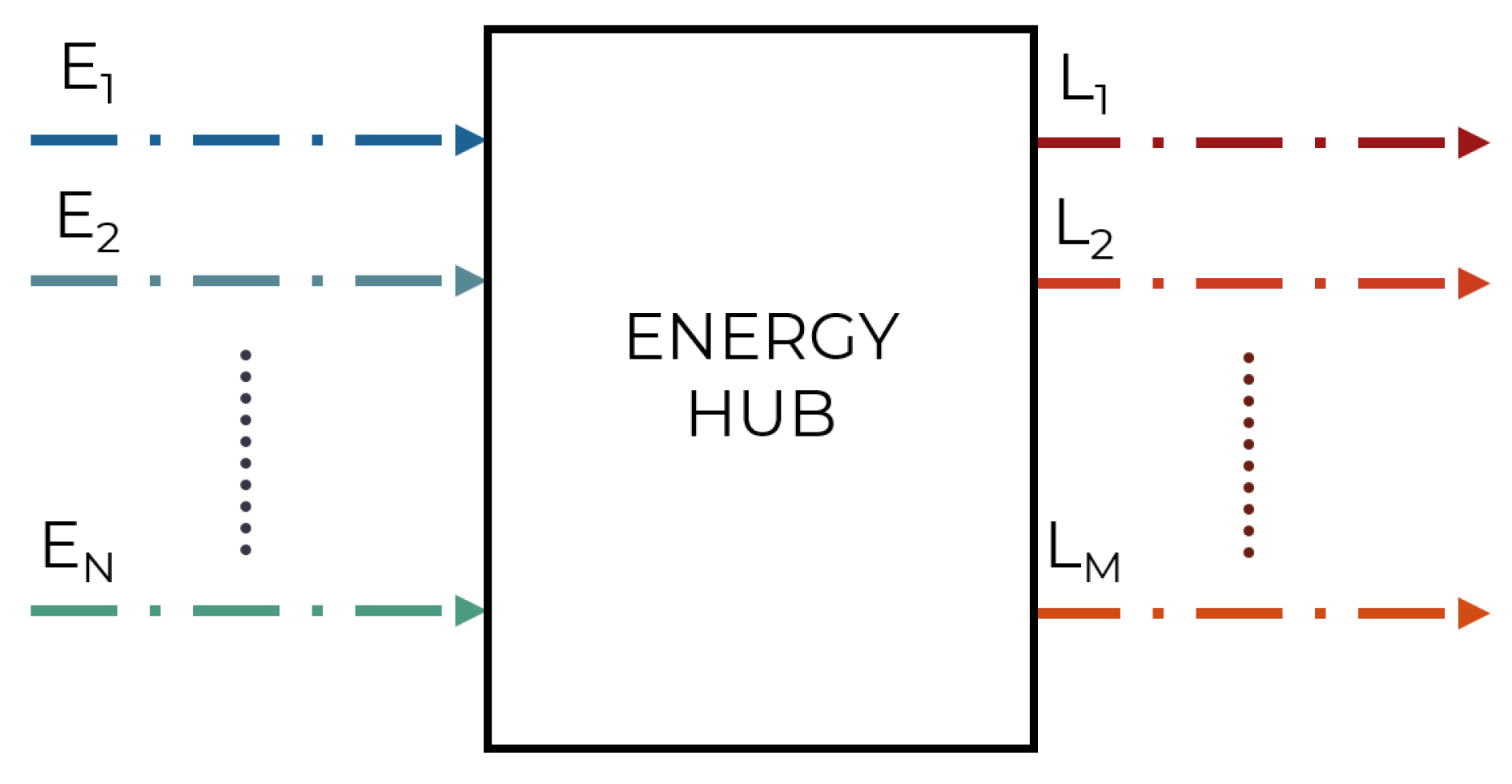
An energy hub can be represented as an open system, with multiple inputs and multiple outputs and consisting of several technologies capable of converting input energy carriers in the required output form.

A general model, considering a steady state system, is represented in Figure 1.

It consists of a series of input energy carriers: $\mathit{E}=[E_1,E_2,...,E_N]$, a series of loads $\mathit{L}=[L_1,L_2,...,L_M]$ and various converting technologies represented by a value of energy conversion efficiency $c_{n,m}$. Input i is connected to output j by the following relation:

$$L_j=c_{i,j}{E}_i$$

(1)

Considering an entire energy hub, the aforementioned relation can be written in matrix form, as a set of linear equations:

$$\left[\begin{array}{c}{L}_1\\ L_2\\ ⋮\\ L_M\end{array}\right]=\left[\begin{array}{cccc}{c}_{1,1}& c_{1,2}& \cdots & c_{1,M}\\ c_{2,1}& c_{2,2}& \cdots & c_{2,M}\\ ⋮& ⋮& \ddots & ⋮\\ c_{N,1}& c_{N,2}& \cdots & c_{N,M}\end{array}\right]\left[\begin{array}{c}{E}_1\\ E_2\\ ⋮\\ E_N\end{array}\right]$$

(2)

The matrix of conversion coefficients can be called the coupling matrix C: its elements, $c_{i,j}$ are zero, if input i is not correlated to output j, or equal to the conversion efficiency of a single device or a proper combination of the efficiencies of multiple devices in case input i and output j are connected. The model can be easily extended to take into account energy storage systems, as described in Reference [8].

2.2. Deterministic Optimal Dispatch

Once the model of an energy hub has been established, a critical problem is how to optimize its operation in order to minimize the operational costs, losses or greenhouse gases emissions.

The problem—referred to as optimal scheduling—can be mathematically formalized by a constrained optimization problem, whose general form is:

$$\begin{array}{cc}\underset{\mathit{x}}{\min }\hfill & f(\mathit{x})\hfill \\ \mathrm{s}.\mathrm{t}.\hfill & g_i(\mathit{x})=0i=1,...,n_g\hfill \\ & h_j(\mathit{x})\le 0,j=1,...,n_h\hfill \end{array}$$

The vector $\mathit{x}$ of decision variables, in this particular case, is the optimal dispatch strategy $\mathit{E}$, while the objective function refers to the criterion chosen to optimize the system.

The equality constraints are linear and they are defined by the model of energy hub previously described:

$$\mathit{L}=\mathit{C}\mathit{P}$$

(3)

The inequality constraints are related to feasible operating ranges, that is, the minimum and maximum values that are allowable for the decision variables:

$$\underline{\mathit{E}}\le \mathit{E}\le \overline{\mathit{E}}$$

(4)

The deterministic optimal dispatch problem considered does not take into account all the uncertainty sources that appear in a real-scenario setting [32,33]:

• Energy prices: Electricity and natural gas prices are uncertain. Depending on the considered energy system, they are characterized by different degrees of volatility, which can be estimated [34].
• Load dynamics: Loads are predictable only with a certain degree of accuracy. Different external factors, such as economic, weather and social aspects, affect their dynamics, thus their behaviour is uncertain.
• Renewable energy generation: Production from solar and wind power are intrinsically uncertain [35].

Hence, a more robust and reliable formulation should be defined in order to properly manage these uncertainty sources. To address this issue, in this paper a novel approach based on Affine Arithmetic is proposed.

3. Affine Arithmetic

In affine arithmetic, a quantity $\widehat{x}$ is represented by an expression of the form [36]:

$$\widehat{x}=x_0+x_1{\epsilon }_1+...+x_n{\epsilon }_n$$

(5)

which is a first-degree polynomial of the variables ${\epsilon }_i$, which are called noise symbols, that are bounded in the interval [−1, 1], and represent independent sources of uncertainty.

The central value of the affine form $\widehat{x}$ is $x_0$, and $x_i$ corresponds to a partial deviation from that value due to effect of the i-th uncertainty source.

Linear mappings for affine forms are defined as follows:

$$\widehat{x}\pm \widehat{y}=x_0\pm y_0+(x_1\pm y_1){\epsilon }_1+(x_2\pm y_2){\epsilon }_2+...+(x_n\pm y_n){\epsilon }_n$$

(6)

$$\alpha \widehat{x}=(\alpha x_0)+(\alpha x_1){\epsilon }_1+(\alpha x_2){\epsilon }_2+...+(\alpha x_n){\epsilon }_n\forall \alpha \in \mathcal{R}$$

(7)

$$\widehat{x}\pm \lambda =(x_0\pm \lambda )+x_1{\epsilon }_1+x_2{\epsilon }_2+...+x_n{\epsilon }_n\forall \lambda \in \mathcal{R}$$

(8)

In the case of a non-linear function of an affine form $f(\widehat{x})$, the result cannot be an affine form itself; hence, it is necessary to approximate the function $f^{\ast }({\epsilon }_1,{\epsilon }_2,...,{\epsilon }_N)$ over its domain to find an affine form that approximates the function.

$$f^{\alpha }({\epsilon }_1,{\epsilon }_2,...,{\epsilon }_N)=z_0+z_1{\epsilon }_1+...z_N{\epsilon }_N$$

(9)

In such a case, a new term that takes into account the approximation error must be introduced and the resulting affine form will be:

$$\widehat{z}=f^{\alpha }({\epsilon }_1,{\epsilon }_2,...,{\epsilon }_N)+z_{N+1}{\epsilon }_{N+1}=z_0+z_1{\epsilon }_1+...z_N{\epsilon }_N+z_{N+1}{\epsilon }_{N+1}$$

(10)

The term $z_{N+1}{\epsilon }_{N+1}$ represents the error defined as:

$$e(z_0+z_1{\epsilon }_1+...+z_N{\epsilon }_N)=f^{\ast }({\epsilon }_1,...,{\epsilon }_N)-f^{\alpha }({\epsilon }_1,...,{\epsilon }_N)$$

(11)

and $z_{N+1}\in {\mathcal{R}}^{+}$ represents an upper bound for its absolute magnitude. Affine Arithmetic has been successfully applied to different problems in power systems, in order to deal with uncertain data, as explained in [37,38], and it can be applied to energy hubs as well. Rather than approximating the non-linear function by introducing a new noise symbol, the so-called endogenous uncertainty, in this paper an alternative approach is adopted.

The main idea is to generalize the basic notion of the affine form, defined in Equation (5), by introducing the concept of extended affine form, which allows a more accurate description of non linear functions based on products between affine forms. This form can be represented by the following:

$$\widehat{\widehat{z}}=\widehat{x}·\widehat{y}=x_0{y}_0+\sum _{i=1}^N(x_i{y}_0+y_i{x}_0){\epsilon }_i+\sum _{i=1}^n{x}_i\sum _{j=1}^n{y}_j{\epsilon }_i{\epsilon }_j=z_0+\sum _{i=1}^N{z}_i{\epsilon }_i+\sum _{i,j=1}^n{z}_{ij}{\epsilon }_{ij}$$

(12)

where the term extended, refers to the presence of the noise symbols ${\epsilon }_{ij}$.

The main complexity in dealing with the extended affine forms is that the upper and lower bounds require the solution of a maximization /minimization problem, mainly:

Upper bound:

$$\begin{array}{c}\sup (\widehat{\widehat{x}})=\underset{{\epsilon }_i}{\max }(x_0+\sum _{i=1}^N{x}_i{\epsilon }_i\sum _{i,j=1}^N{x}_{i,j}{\epsilon }_{i,j})\hfill \\ -1\le {\epsilon }_i\le 1\hfill \end{array}$$

(13)

Lower bound:

$$\begin{array}{c}\inf (\widehat{\widehat{x}})=\underset{{\epsilon }_i}{\min }(x_0+\sum _{i=1}^N{x}_i{\epsilon }_i+\sum _{i,j=1}^N{x}_{i,j}{\epsilon }_{i,j})\hfill \\ -1\le {\epsilon }_i\le 1\hfill \end{array}$$

(14)

Radius:

$$rad(\widehat{\widehat{x}})=\frac{\sup (\widehat{\widehat{x}})-\inf (\widehat{\widehat{x}})}{2}$$

(15)

According to these definitions, the following mathematical operators can be inferred:

Equality operator:

$$\widehat{\widehat{x}}=\widehat{\widehat{y}}\iff \left\{\begin{array}{c}{x}_0=y_0\hfill \\ x_i=y_i\forall i=1,...,N\hfill \\ x_{ij}=y_{ij}\forall i,j=1,...,N\hfill \end{array}\right.$$

(16)

Inequality operator:

$$\widehat{\widehat{x}}\le \widehat{\widehat{y}}\iff \sup (\widehat{\widehat{x}})\le \inf (\widehat{\widehat{y}})$$

(17)

Minimization operator:

$$\underset{x_i,x_{ij}}{\min }\widehat{\widehat{x}}\iff \underset{x_i,x_{ij}}{\min }(x_0,rad(\widehat{\widehat{x}}))$$

(18)

By analysing the last operator, it is worth observing that the minimization of an extended affine form requires the solution of a min-max optimization problem. The nature of the problem describes the risk attitude of the analyst, which can decide to minimize the central value, or the radius, if a reliable solution is required. A direct correlation with the theory of robust optimization can be inferred and will be explored in future papers.

A simple numerical example is provided to illustrate the extended affine arithmetic-based optimization. Consider the following two affine forms as decision variables:

$$\begin{array}{c}\hfill \widehat{x}=x_0+x_1{\epsilon }_1+x_2{\epsilon }_2\\ \hfill \widehat{y}=y_0+y_1{\epsilon }_1+y_2{\epsilon }_2\end{array}$$

(19)

And $\widehat{\widehat{z}}=\widehat{x}\widehat{y}$ as the optimization function.

The constrained optimization problem to be solved is the following:

$$\begin{array}{cc}\underset{\widehat{x},\widehat{y}}{\min }\hfill & rad(\widehat{\widehat{z}})\hfill \\ s.t.\hfill & \widehat{x}+\widehat{y}=20+5{\epsilon }_1+7{\epsilon }_2\hfill \\ & 0\le \widehat{x}\le 20\hfill \\ & 0\le \widehat{y}\le 10\hfill \end{array}$$

(20)

This problem can be rewritten as a simple deterministic optimization by writing the constraints as:

$$\begin{array}{cc}\underset{x_0,x_1,x_2,y_0,y_1,y_2}{\min }& rad(\widehat{\widehat{z}})\hfill \\ s.t.& x_0+y_0=20\hfill \\ & x_1+y_1=5\hfill \\ & x_2+y_2=7\hfill \\ & x_0+\sum _{i=1}^2\left|x_i\right|\le 30\hfill \\ & y_0+\sum _{i=1}^2\left|y_i\right|\le 20\hfill \\ & x_0-\sum _{i=1}^2\left|x_i\right|\ge 0\hfill \\ & y_0-\sum _{i=1}^2\left|y_i\right|\ge 0\hfill \end{array}$$

(21)

The affine forms that solve the previously described optimization problem are shown in

Table 1. Simple numerical example of Extended Affine Arithmetic.

Affine Form Values	x	y
Central value	10.04	9.96
P. dev. 1	2.51	2.5
P. dev. 2	3.52	3.48

:

Extended Affine Arithmetic can be used to solve the optimal scheduling problem of an energy hub in the presence of multiple uncertainty sources. As previously explained, three main uncertain input variables are considered in this study, namely energy prices $C_i$, loads demand $L_j$ and renewable energy generation $E_{ren,k}$, which are expressed by the following affine forms.

$$\begin{array}{c}{\widehat{C}}_i=C_{p,0}+{\epsilon }_{C_p}\forall p=1,...N\hfill \\ {\widehat{L}}_j=L_{j,0}+{\epsilon }_{L_j}\forall j=1,...M\hfill \\ {\widehat{E}}_{ren,k}=E_{ren,k,0}+{\epsilon }_{E_{ren,k}}\forall k=1,...,P\hfill \end{array}$$

(22)

Once the uncertainty sources are established, decision variables $E_i$ can be expressed as the sum of a central value and a series of partial deviations equal to the number of uncertainty sources considered:

$${\widehat{E}}_i=E_{i,0}+\sum _{p=1}^N{E}_{i,p}{\epsilon }_{C_p}+\sum _{j=1}^M{E}_{i,j}{\epsilon }_{L_j}+\sum _{k=1}^P{E}_{i,k}{\epsilon }_{E_{ren,k}}\forall i=1,...,N$$

(23)

where N is the number of input energy carriers, that is, the decision variables, and thus the number of uncertain costs considered, M is the number of loads and P the renewable energy generators. The total number of uncertainty sources and thus partial deviations of a decision variable in a particular problem is $N+P+M$.

The total cost, in this case, is an extended affine form with respect to the noise symbols ${\epsilon }_i$ and it is equal to the following expression:

$$C_{tot}=\sum _{i=1}^N{\widehat{C}}_i{\widehat{E}}_i=\sum _{i=1}^N(C_{i,0}+{\epsilon }_{C_i})·(E_{i,0}+\sum _{p=1}^N{E}_{i,p}{\epsilon }_{C_p}+\sum _{j=1}^M{E}_{i,j}{\epsilon }_{L_j}+\sum _{k=1}^P{E}_{i,k}{\epsilon }_{E_{ren,k}})$$

(24)

When formulating an optimization problem, different criteria can be chosen depending on the risk attitude of the analyst. A reliable solution can be found by minimizing the radius of $C_{tot}$, that is, by finding the decision variables $\widehat{E_i}$ that minimize its upper value with respect to every ${\epsilon }_i$, where the upper value can be found by solving a sub-level optimization problem with respect to $\mathit{\epsilon }$. In this case, the decision variables will be affine forms $\widehat{E_i}$, thus, in the optimization problem, the values to be found will be $N+N\ast Q$: $\mathit{E}=\left\{E_{i,j}\right\}\forall i=1,...,N,j=0,...,Q$.

The equality constraints in affine forms can be reformulated as a system of deterministic constraints, each associated to a noise symbol, as shown in the following example. Assuming only one uncertain load L and Q total uncertain sources:

$$L_0+L_1{\epsilon }_1=\sum _{i=1}^N{\eta }_i(E_{i,0}+E_{i,1}{\epsilon }_1+E_{i,2}{\epsilon }_2+...+E_{i,Q}{\epsilon }_Q)$$

(25)

The previous constraint becomes a series of Q deterministic equality constraints:

$$\begin{array}{c}{L}_0=\sum _{i=1}^N{\eta }_i{E}_{i,0}\\ L_1=\sum _{i=1}^N{\eta }_i{E}_{i,1}\\ 0=\sum _{i=1}^N{\eta }_i{E}_{i,2}\\ ⋮\\ 0=\sum _{i=1}^N{\eta }_i{E}_{i,Q}\end{array}$$

(26)

Thus, for M loads and Q uncertainty sources, the total number of equality constraints will be $M+Q\ast M$, and it can be written in matrix form as $\widehat{\mathit{L}}$=$\mathit{C}\widehat{\mathit{E}}$. The inequality constraints can be written in the following form, where $|E_{i,j}|$ represents the absolute value of the j-th partial deviation related to the i-th decision variable, $\underline{E_i}$ is the minimum and $\overline{E_i}$, the maximum value:

$$E_{i,0}-\sum _{j=1}^Q\left|E_{i,j}\right|\ge \underline{E_i}\forall i=1,...,N$$

(27)

$$E_{i,0}+\sum _{j=1}^Q\left|E_{i,j}\right|\le \overline{E_i}\forall i=1,...,N$$

(28)

Finally, the whole problem can be written as the following optimization problem:

$$\begin{array}{cc}\underset{\mathit{E}}{\min }\hfill & rad(C_{tot}(\mathit{E}))\hfill \\ s.t.\hfill & \widehat{\mathit{L}}=\mathit{C}\widehat{\mathit{E}}\hfill \\ & E_{i,0}-\sum _{j=1}^Q\left|E_{i,j}\right|\ge \underline{E_i}\forall i=1,...,N\hfill \\ & E_{i,0}+\sum _{j=1}^Q\left|E_{i,j}\right|\le \overline{E_i}\forall i=1,...,N\hfill \end{array}$$

(29)

The solution of this problem is represented by a series of affine forms $\widehat{E_i}$ which minimizes the radius of the total cost and is guaranteed to satisfy the constraints. Such affine forms have a strategic importance for the efficient scheduling of an energy hub, since they enclose the value of the objective function in a known range, which is guaranteed to contain the actual value despite the effects of data uncertainty.

Once the affine forms are known, the real-time dispatch values $E_i$ can be computed by calculating the noise symbols associated to the deterministic values $C_{p,real},L_{j,real},E_{ren,k,real}$:

$${\widehat{E}}_i=E_{i,0}+\sum _{i=1}^N{E}_{i,p}{\epsilon }_{C_p}^{\ast }+\sum _{j=1}^M{E}_{i,j}{\epsilon }_{L_j}^{\ast }+\sum _{k=1}^P{E}_{i,k}{\epsilon }_{E_{ren,k}}^{\ast }\forall i=1,...,N$$

(30)

$$\begin{array}{c}{\epsilon }_{C_p}^{\ast }=\frac{C_{p,real}-C_{p,0}}{C_{p,1}}\forall p=1,...,N\hfill \\ {\epsilon }_{L_j}^{\ast }=\frac{L_{j,real}-L_{j,0}}{L_{j,1}}\forall j=1,...,Q\hfill \\ {\epsilon }_{E_{ren,k}}^{\ast }=\frac{E_{ren,k,real}-E_{ren,k,0}}{E_{ren,k,1}}\forall k=1,...,P\hfill \end{array}$$

(31)

4. Case Study

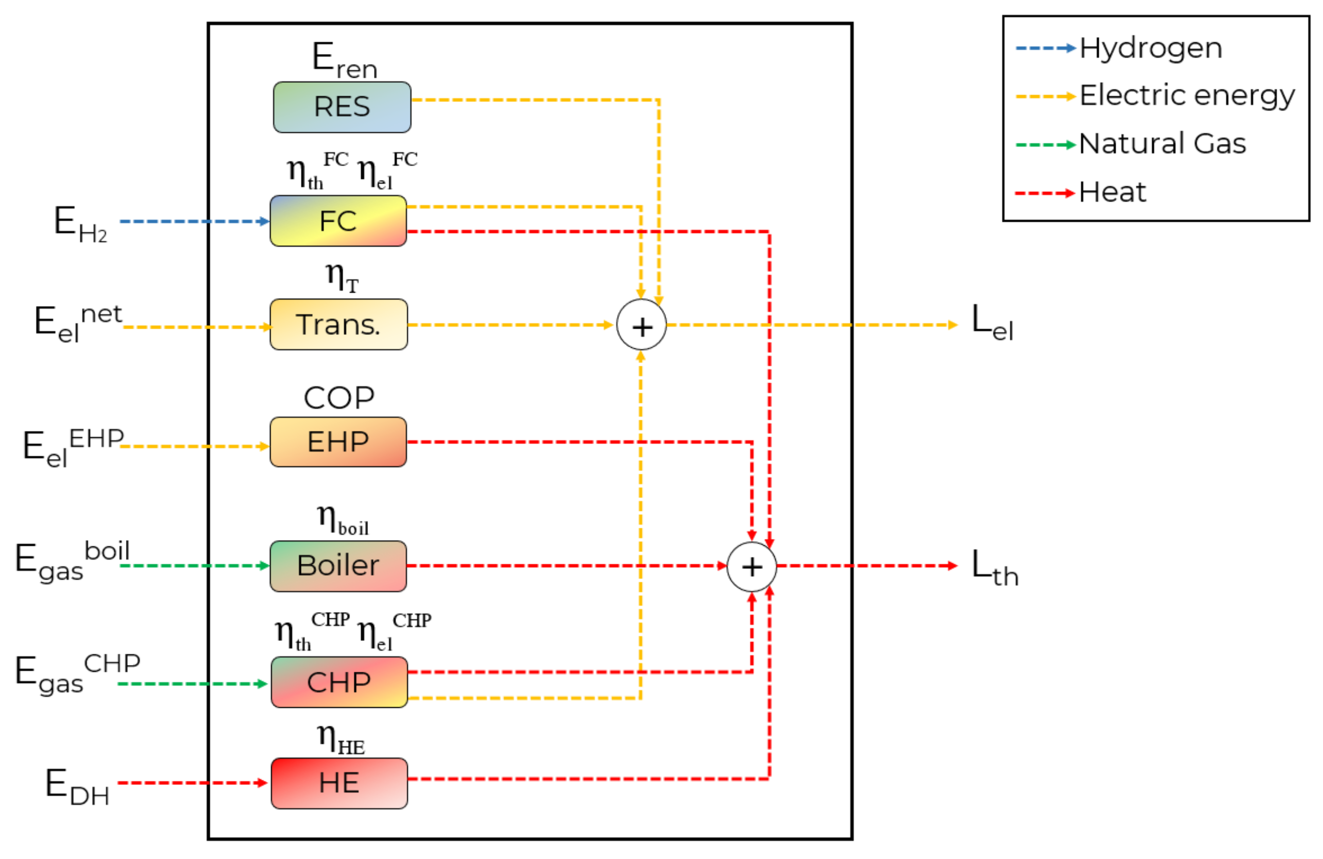
To show the effectiveness of the proposed technique, in this paper, the energy hub shown in Figure 2 is considered. It consists of six converters, a thermal load $L_{th}$, an electrical load $L_{el}$ and a renewable energy generator $E_{ren}$. The input carriers are electric energy, natural gas, hydrogen and district heating although they are divided into six different inputs in order to keep the mathematical model linear: $E_{H_2},E_{el}^{net},E_{el}^{EHP},E_{gas}^{boil},E_{gas}^{CHP},E_{DH}$.

The converters considered are:

• Transformer: it connects the electric energy input from the grid to the electric load, ${\eta }_T=0.98$.
• Electric Heat Pumps (EHP): they serve the thermal load by efficiently converting input electric energy, the coefficient of performance (COP) is set to $2.5$.
• Boilers: they simply work by burning natural gas and serving thermal load, ${\eta }_{boil}=0.8$.
• Combined Heat and Power (CHP): such elements serve both loads, and they are fed by natural gas. The efficiencies for electric and thermal conversion are: ${\eta }_{el}^{CHP}=0.35$, ${\eta }_{th}^{CHP}=0.405$.
• Fuel Cells (FC): they can produce both electric energy and heat by converting hydrogen ${\eta }_{el}^{FC}=0.35$, ${\eta }_{th}^{FC}=0.45$.
• Heat Exchangers (HE): thermal load can be served by district heating, through the heat exchangers, whose heat transfer efficiency is set to ${\eta }_{HE}=0.9$.

The energy balance equations can be written in matrix form as:

$$\left[\begin{array}{ccccccc}1& {\eta }_{el}^{FC}& {\eta }_T& 0& 0& {\eta }_{el}^{CHP}& 0\\ 0& {\eta }_{th}^{FC}& 0& COP& {\eta }_{boil}& {\eta }_{th}^{CHP}& {\eta }_{HE}\end{array}\right]·\left[\begin{array}{c}{E}_{ren}\\ E_{H_2}\\ E_{el}^{net}\\ E_{el}^{EHP}\\ E_{gas}^{boil}\\ E_{gas}^{CHP}\\ E_{DH}\end{array}\right]=\left[\begin{array}{c}{L}_{el}\\ L_{th}\end{array}\right]$$

(32)

The sources of uncertainty considered in this case are related to electric energy and natural gas costs, loads and renewable energy production, while hydrogen and district heating costs are supposed to be known with certainty, thus five affine forms and two scalar values are defined as input.

$$\begin{array}{c}{\widehat{L}}_{el}=L_{el,0}+L_{el,1}{\epsilon }_{L_{el}}\hfill \\ {\widehat{L}}_{th}=L_{th,0}+L_{th,1}{\epsilon }_{L_{th}}\hfill \\ {\widehat{C}}_{el}=C_{el,0}+C_{el,1}{\epsilon }_{C_{el}}\hfill \\ {\widehat{C}}_{gas}=C_{gas,0}+C_{gas,1}{\epsilon }_{C_{gas}}\hfill \\ {\widehat{E}}_{ren}=E_{ren,0}+E_{ren,1}{\epsilon }_{E_{ren}}\hfill \\ C_{H_2}=C_{H_2,0}\hfill \\ C_{DH}=C_{DH,0}\hfill \end{array}$$

(33)

The central values and the partial deviations considered in this case study are described in

Table 2. Central value and partial deviations of each uncertain quantity.

Affine Form Values	${\mathit{C}}_{\mathit{el}}$ (€/MWh)	${\mathit{C}}_{\mathit{gas}}$ (€/MWh)	${\mathit{L}}_{\mathit{el}}$ (MWh)	${\mathit{L}}_{\mathit{th}}$ (MWh)	${\mathit{E}}_{\mathit{ren}}$ (MWh)
Central value	60	44	20	20	0
Uncertainty	8	4.4	0.5	0.9	2

.

Since the renewable energy production is considered completely uncertain, the central value is assumed to be equal to the partial deviation.

Since there are five uncertainty sources, the affine forms of the decision variables are described by the following:

$$\begin{array}{c}{\widehat{E}}_{el}^{net}=E_{el,0}^{net}+\sum _{i=1}^5{E}_{el,i}^{net}{\epsilon }_i\hfill \\ {\widehat{E}}_{el}^{EHP}=E_{el,0}^{EHP}+\sum _{i=1}^5{E}_{el,i}^{EHP}{\epsilon }_i\hfill \\ {\widehat{E}}_{gas}^{boil}=E_{gas,0}^{boil}+\sum _{i=1}^5{E}_{gas,i}^{boil}{\epsilon }_i\hfill \\ {\widehat{E}}_{gas}^{CHP}=E_{gas,0}^{CHP}+\sum _{i=1}^5{E}_{gas,i}^{CHP}{\epsilon }_i\hfill \\ {\widehat{E}}_{H_2}=E_{H_2,0}+\sum _{i=1}^5{E}_{H_2,i}{\epsilon }_i\hfill \\ {\widehat{E}}_{DH}=E_{DH,0}+\sum _{i=1}^5{E}_{DH,i}{\epsilon }_i\hfill \end{array}$$

(34)

The total costs are $C_{tot}=C_{el,tot}+C_{gas,tot}$, where the single components are calculated as follows:

$$\begin{array}{c}{C}_{tot}=(C_{el,0}+C_{el,1}{\epsilon }_3)·[(E_{el,0}^{net}+E_{el,0}^{EHP})+\sum _{i=1}^5{\epsilon }_i(E_{el,i}^{net}+E_{el,i}^{EHP})]\hfill \\ +(C_{gas,0}+C_{gas,1}{\epsilon }_4)·[(E_{gas,0}^{CHP}+E_{gas,0}^{boil})+\sum _{i=1}^5{\epsilon }_i(E_{gas,i}^{CHP}+E_{gas,i}^{boil})]\hfill \\ +C_{H_2,0}·[E_{H_2,0}+\sum _{i=1}^5{\epsilon }_i{E}_{H_2,i}]+C_{DH,0}·[E_{DH,0}+\sum _{i=1}^5{\epsilon }_i{E}_{DH,i}]\hfill \end{array}$$

(35)

The equality constraints, related to the energy balance on the energy hub are:

$$L_{el,0}+L_{el,1}{\epsilon }_1={\eta }^{net}(E_{el,0}^{net}+\sum _{i=1}^5{E}_{el,i}^{net}{\epsilon }_i)+{\eta }_{el}^{CHP}(E_{gas,0}^{CHP}+\sum _{i=1}^5{E}_{gas,i}^{CHP}{\epsilon }_i)+{\eta }_{el}^{FC}(E_{H_2,0}+\sum _{i=1}^5{E}_{H_2,i}{\epsilon }_i)$$

(36)

$$\begin{array}{c}{L}_{th,0}+L_{th,1}{\epsilon }_2=COP(E_{el,0}^{EHP}+\sum _{i=1}^5{E}_{el,i}^{EHP}{\epsilon }_i)+{\eta }_{gas}(E_{gas,0}^{boil}+\sum _{i=1}^5{E}_{gas,i}^{boil}{\epsilon }_i)\hfill \\ +{\eta }_{th}^{CHP}(E_{gas,0}^{CHP}+\sum _{i=1}^5{E}_{gas,i}^{CHP}{\epsilon }_i)+{\eta }_{th}^{FC}(E_{H_2,0}+\sum _{i=1}^5{E}_{H_2,i}{\epsilon }_i)+{\eta }_{HE}(E_{DH,0}+\sum _{i=1}^5{\epsilon }_i{E}_{DH,i})\hfill \end{array}$$

(37)

The inequality constraints describe the allowable operating points of each technology, that is, $\forall i$:

$$\begin{array}{c}{E}_{el,0}^{net}-\sum _{i=1}^5|E_{el,i}^{net}|\ge E_{el,min}^{net}{E}_{el,0}^{net}+\sum _{i=1}^5\left|E_{el,i}^{net}\right|\le E_{el,max}^{net}\hfill \\ E_{el,0}^{EHP}-\sum _{i=1}^5|E_{el,i}^{EHP}|\ge E_{el,min}^{EHP}{E}_{el,0}^{EHP}+\sum _{i=1}^5\left|E_{el,i}^{EHP}\right|\le E_{el,max}^{EHP}\hfill \\ E_{gas,0}^{boil}-\sum _{i=1}^5|E_{gas,i}^{boil}|\ge E_{gas,min}^{boil}{E}_{gas,0}^{boil}+\sum _{i=1}^5\left|E_{gas,i}^{boil}\right|\le E_{gas,max}^{boil}\hfill \\ E_{gas,0}^{CHP}-\sum _{i=1}^5|E_{gas,i}^{CHP}|\ge E_{gas,min}^{CHP}{E}_{gas,0}^{CHP}+\sum _{i=1}^5\left|E_{gas,i}^{CHP}\right|\le E_{gas,max}^{CHP}\hfill \\ E_{H_2,0}-\sum _{i=1}^5|E_{H_2,i}|\ge E_{H_2,min}{E}_{H_2,0}+\sum _{i=1}^5\left|E_{H_2,i}\right|\le E_{H_2,max}\hfill \\ E_{DH,0}-\sum _{i=1}^5|E_{DH,i}|\ge E_{DH,min}{E}_{DH,0}+\sum _{i=1}^5\left|E_{DH,i}\right|\le E_{DH,max}\hfill \end{array}$$

(38)

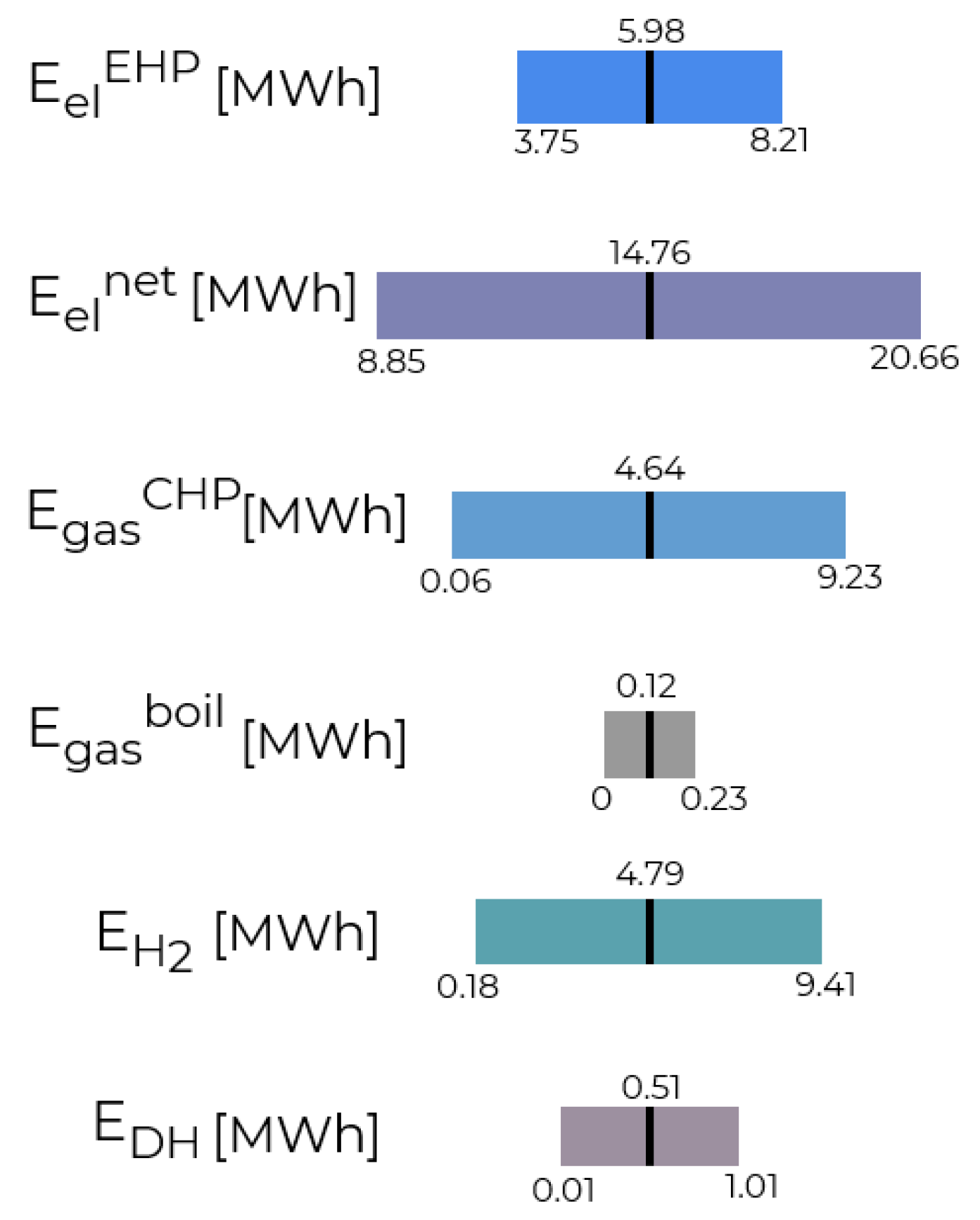
The affine forms obtained as a solution to the aforementioned problem are described in

Table 3. Central value and partial deviations for each affine form.

Affine Form Values	${\mathit{E}}_{\mathit{el},\mathit{i}}^{\mathit{EHP}}$ (MWh)	${\mathit{E}}_{\mathit{el},\mathit{i}}^{\mathit{net}}$ (MWh)	${\mathit{E}}_{\mathit{gas},\mathit{i}}^{\mathit{CHP}}$ (MWh)	${\mathit{E}}_{\mathit{gas},\mathit{i}}^{\mathit{boil}}$ (MWh)	${\mathit{E}}_{{\mathit{H}}_2,\mathit{i}}$ (MWh)	${\mathit{E}}_{\mathit{DH},\mathit{i}}$ (MWh)
Central value	5.98	14.76	4.65	0.122	4.79	0.51
P. dev. 1	0.03	0.57	0.211	−0.04	−0.37	0
P. dev. 2	0.64	0.58	−1.31	0	−0.13	0.01
P. dev. 3	0.79	1.29	−1.18	−0.07	−2.27	−0.36
P. dev. 4	0.44	0.84	−1.85	0	−0.25	−0.08
P. dev. 5	−0.31	−2.62	0.03	0	1.59	0.04

, which lists the central value and the partial deviations of each decision variable. Figure 3 shows the resulting intervals. The total cost, depending on the value of gas, electric energy, hydrogen and district heating prices, loads and renewable energy production is guaranteed to stay in the following range: $C_{tot}=[1439,2003]$ €.

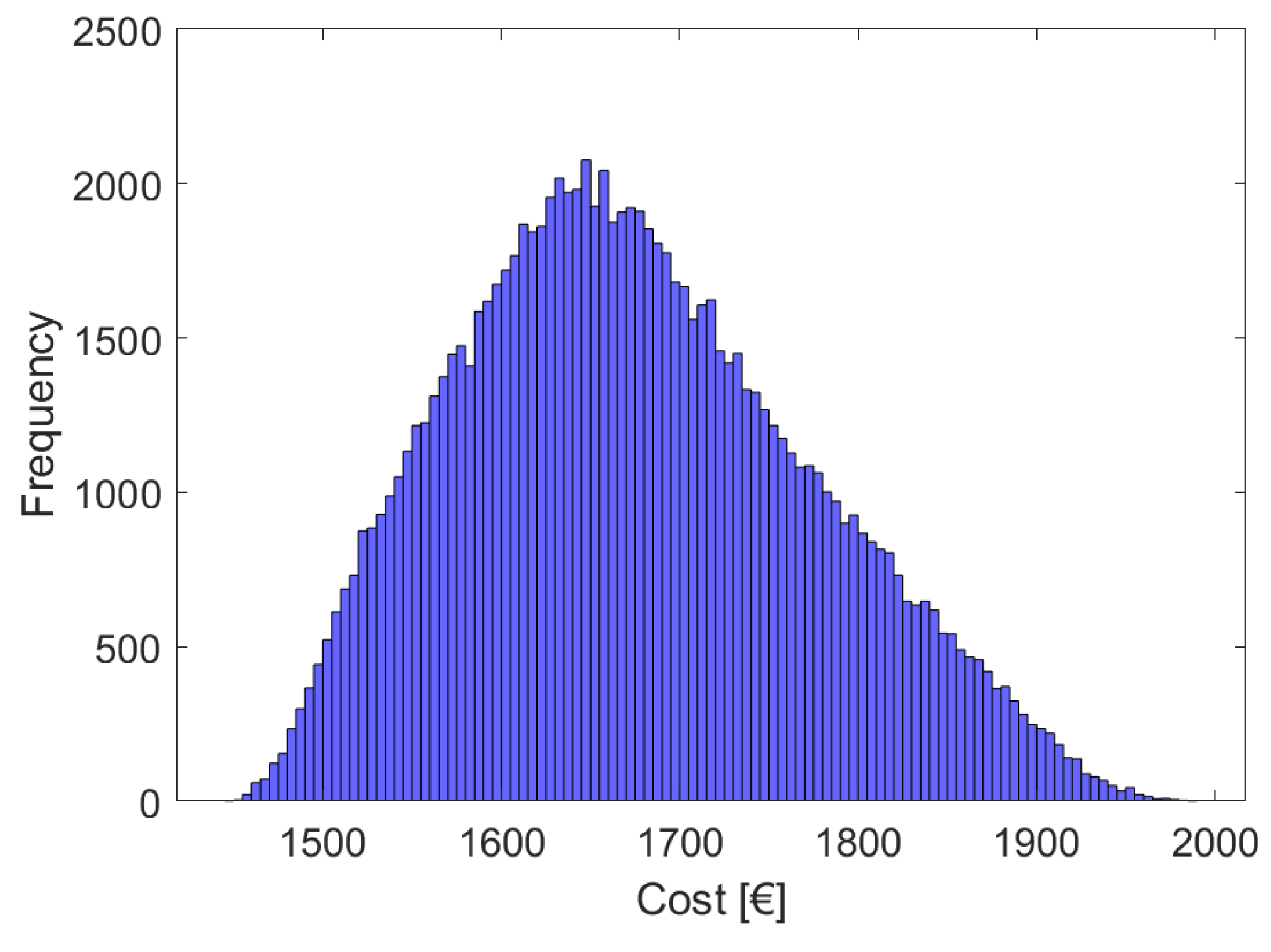
To assess the reliability of the solution found, a Montecarlo simulation has been performed. Considering 100,000 random samples, the results related to cost are shown in Figure 4. It can be seen that the total cost remains in the calculated range for each possible scenario, including the worst case instance of the considered uncertainty sources.

Results were compared to stochastic and robust optimization: in the first case the cost was in the range: $C_{tot}=[1347,1996]$ €, while considering the worst case scenario, the cost was $C_{tot}=2021$ €.

The extended affine arithmetic method provides results that are coherent with similar optimization techniques in the presence of uncertainty, although such a method provides more flexible and computationally more efficient results.

In the case of extended affine arithmetic optimization, once the real-time values of the uncertain quantities are known: ${\overline{L}}_{el},{\overline{L}}_{th},{\overline{C}}_{el},{\overline{C}}_{th},{\overline{E}}_{ren}$, the value of the noise symbol can be calculated as:

$$\begin{array}{c}{ϵ}_1^{\ast }=\frac{{\overline{L}}_{el}-L_{el,0}}{L_{el,1}}\hfill \\ {ϵ}_2^{\ast }=\frac{{\overline{L}}_{th}-L_{th,0}}{L_{th,1}}\hfill \\ {ϵ}_3^{\ast }=\frac{{\overline{C}}_{el}-C_{el,0}}{C_{el,1}}\hfill \\ {ϵ}_4^{\ast }=\frac{{\overline{C}}_{gas}-C_{gas,0}}{C_{gas,1}}\hfill \\ {ϵ}_5^{\ast }=\frac{{\overline{E}}_{ren}-E_{ren,0}}{E_{ren,1}}\hfill \end{array}$$

(39)

Thus, every decision variable and the cost associated to a certain event can be precisely calculated for each scenario without solving a new optimization problem.

For example, consider a scenario in which the values of the input variables are the following: $L_{el}=19.82$ MWh, $L_{th}=19.63$ MWh, $C_{el}=60.93$ €/MWh, $C_{gas}=40.19$ €/MWh and $E_{ren}$ = 0.27 MWh.

In this case: ${\epsilon }_1^{\ast }=-0.348$, ${\epsilon }_2^{\ast }=-0.407$, ${\epsilon }_3^{\ast }=0.116$, ${\epsilon }_4^{\ast }=-0.865$, ${\epsilon }_5^{\ast }=-0.862$.

The corresponding decision variables associated to this scenario are obtained by substituting each noise symbol ${\epsilon }_i^{\ast }$ in the resulting affine forms:

$${\widehat{E}}_k^j=E_{k,0}^j+\sum _{i=1}^5{E}_{k,i}^j{\epsilon }_i^{\ast }$$

(40)

Hence obtaining the following values: $E_{el}^{net}=16$ MWh, $E_{el}^{EHP}$=5.68 MWh, $E_{gas}^{boil}=0.12$ MWh, $E_{gas}^{CHP}=6.54$ MWh, $E_{H_2}=3.55$ MWh, $E_{D_H}=0.5$ MWh.

5. Conclusions

This paper presented a novel methodology based on extended Affine Arithmetic to reliably manage multiple uncertainties in the optimal scheduling of an energy hub.

After introducing the energy hub model and the main sources of uncertainty affecting the optimal scheduling problem, a description of generalized Affine Arithmetic has been given. Then, this new methodology was applied to an energy hub’s optimal scheduling problem in the presence of uncertainty and a novel mathematical formulation was established.

The proposed technique represents a strategic tool for an analyst whose aim is to minimize operational costs of an energy hub. The affine forms calculated offer a powerful tool for short time planning and real-time dispatching. The case study’s results, assuming that the uncertainty interval of input variables is known, showed the robustness of the obtained solution. Furthermore, given a decision variable expressed as an affine form and its associated range, the analyst can properly adjust his decisions to match the expected robustness level.

Future work on this subject may focus on the application of extended Affine Arithmetic to manage uncertainty for different energy hub models, including storage systems and thus inter-temporal constraints, as far as in exploring a formal connection between extended Affine Arithmetic and robust optimization.

References

- Ackermann, T.; Andersson, G.; Söder, L. Distributed generation: A definition. Electr. Power Syst. Res. 2001, 57, 195–204. [Google Scholar] [CrossRef]
- Mancarella, P. MES (multi-energy systems): An overview of concepts and evaluation models. Energy 2014, 65, 1–17. [Google Scholar] [CrossRef]
- Geidl, M.; Koeppel, G.; Favre-Perrod, P.; Klockl, B.; Andersson, G.; Frohlich, K. Energy hubs for the future. IEEE Power Energy Mag. 2006, 5, 24–30. [Google Scholar] [CrossRef]
- Krause, T.; Andersson, G.; Frohlich, K.; Vaccaro, A. Multiple-energy carriers: Modeling of production, delivery, and consumption. Proc. IEEE 2010, 99, 15–27. [Google Scholar] [CrossRef]
- Mohammadi, M.; Noorollahi, Y.; Mohammadi-Ivatloo, B.; Yousefi, H. Energy hub: From a model to a concept—A review. Renew. Sustain. Energy Rev. 2017, 80, 1512–1527. [Google Scholar] [CrossRef]
- Ma, T.; Wu, J.; Hao, L.; Yan, H.; Li, D. A real time pricing scheme for energy management in integrated energy systems: A stackelberg game approach. Energies 2018, 11, 2858. [Google Scholar] [CrossRef]
- Qi, F.; Wen, F.; Liu, X.; Salam, M. A residential energy hub model with a concentrating solar power plant and electric vehicles. Energies 2017, 10, 1159. [Google Scholar] [CrossRef]
- Brahman, F.; Honarmand, M.; Jadid, S. Optimal electrical and thermal energy management of a residential energy hub, integrating demand response and energy storage system. Energy Build. 2015, 90, 65–75. [Google Scholar] [CrossRef]
- Moghaddam, I.G.; Saniei, M.; Mashhour, E. A comprehensive model for self-scheduling an energy hub to supply cooling, heating and electrical demands of a building. Energy 2016, 94, 157–170. [Google Scholar] [CrossRef]
- Wu, R.; Mavromatidis, G.; Orehounig, K.; Carmeliet, J. Multiobjective optimisation of energy systems and building envelope retrofit in a residential community. Appl. Energy 2017, 190, 634–649. [Google Scholar] [CrossRef]
- Orehounig, K.; Evins, R.; Dorer, V. Integration of decentralized energy systems in neighbourhoods using the energy hub approach. Appl. Energy 2015, 154, 277–289. [Google Scholar] [CrossRef]
- Almassalkhi, M.; Hiskens, I. Optimization framework for the analysis of large-scale networks of energy hubs. In Proceedings of the Power Systems Computation Conference, Stockholm, Sweden, 22–26 August 2011. [Google Scholar]
- Ha, T.; Zhang, Y.; Hao, J.; Thang, V.; Li, C.; Cai, Z. Energy hub’s structural and operational optimization for minimal energy usage costs in energy systems. Energies 2018, 11, 707. [Google Scholar] [CrossRef]
- Zhong, Y.; Xie, D.; Zhai, S.; Sun, Y. Day-ahead hierarchical steady state optimal operation for integrated energy system based on energy hub. Energies 2018, 11, 2765. [Google Scholar] [CrossRef]
- Chen, Y.; Wang, Y.; Ma, J. Multi-objective optimal energy management for the integrated electrical and natural gas network with combined cooling, heat and power plants. Energies 2018, 11, 734. [Google Scholar] [CrossRef]
- Parisio, A.; Del Vecchio, C.; Vaccaro, A. A robust optimization approach to energy hub management. Int. J. Electr. Power Energy Syst. 2012, 42, 98–104. [Google Scholar] [CrossRef]
- Pazouki, S.; Haghifam, M.R.; Moser, A. Uncertainty modeling in optimal operation of energy hub in presence of wind, storage and demand response. Int. J. Electr. Power Energy Syst. 2014, 61, 335–345. [Google Scholar] [CrossRef]
- Canfora, G.; Troiano, L. The importance of dealing with uncertainty in the evaluation of software engineering methods and tools. In Proceedings of the 14th International Conference on Software Engineering and Knowledge Engineering, Ischia, Italy, 15–19 July 2002; ACM: New York, NY, USA, 2002; pp. 691–698. [Google Scholar]
- Vahid-Pakdel, M.; Nojavan, S.; Mohammadi-Ivatloo, B.; Zare, K. Stochastic optimization of energy hub operation with consideration of thermal energy market and demand response. Energy Convers. Manag. 2017, 145, 117–128. [Google Scholar] [CrossRef]
- Najafi, A.; Marzband, M.; Mohamadi-Ivatloo, B.; Contreras, J.; Pourakbari-Kasmaei, M.; Lehtonen, M.; Godina, R. Uncertainty-based models for optimal management of energy hubs considering demand response. Energies 2019, 12, 1413. [Google Scholar] [CrossRef]
- Rakipour, D.; Barati, H. Probabilistic optimization in operation of energy hub with participation of renewable energy resources and demand response. Energy 2019, 173, 384–399. [Google Scholar] [CrossRef]
- Sanjani, K.; Vahabzad, N.; Nazari-Heris, M.; Mohammadi-ivatloo, B. A robust-stochastic approach for energy transaction in energy hub under uncertainty. In Robust Optimal Planning and Operation of Electrical Energy Systems; Springer: Cham, Switzerland, 2019; pp. 219–232. [Google Scholar]
- Najafi-Ghalelou, A.; Nojavan, S.; Zare, K.; Mohammadi-Ivatloo, B. Robust scheduling of thermal, cooling and electrical hub energy system under market price uncertainty. Appl. Therm. Eng. 2019, 149, 862–880. [Google Scholar] [CrossRef]
- Mukherjee, U.; Maroufmashat, A.; Narayan, A.; Elkamel, A.; Fowler, M. A stochastic programming approach for the planning and operation of a power to gas energy hub with multiple energy recovery pathways. Energies 2017, 10, 868. [Google Scholar] [CrossRef]
- Fouskakis, D.; Draper, D. Stochastic optimization: A review. Int. Stat. Rev. 2002, 70, 315–349. [Google Scholar] [CrossRef]
- La Scala, M.; Vaccaro, A.; Zobaa, A. A goal programming methodology for multiobjective optimization of distributed energy hubs operation. Appl. Therm. Eng. 2014, 71, 658–666. [Google Scholar] [CrossRef] [Green Version]
- Vaccaro, A.; Pisani, C.; Zobaa, A.F. Affine arithmetic-based methodology for energy hub operation-scheduling in the presence of data uncertainty. IET Gener. Transm. Distrib. 2015, 9, 1544–1552. [Google Scholar] [CrossRef]
- De Figueiredo, L.H.; Stolfi, J. Affine arithmetic: Concepts and applications. Numer. Algorithms 2004, 37, 147–158. [Google Scholar] [CrossRef]
- Krämer, W. Generalized Intervals and the Dependency Problem. Available online: https://onlinelibrary.wiley.com/doi/pdf/10.1002/pamm.200610322 (accessed on 23 June 2019).
- Neumaier, A. The wrapping effect, ellipsoid arithmetic, stability and confidence regions. In Validation Numerics; Springer: Vienna, Austria, 1993; pp. 175–190. [Google Scholar]
- Bilotta, G. Self-verified extension of affine arithmetic to arbitrary order. Le Matematiche 2008, 63, 15–30. [Google Scholar]
- Soroudi, A.; Amraee, T. Decision making under uncertainty in energy systems: State of the art. Renew. Sustain. Energy Rev. 2013, 28, 376–384. [Google Scholar] [CrossRef]
- Ghasemi, A.; Banejad, M.; Rahimiyan, M. Integrated energy scheduling under uncertainty in a micro energy grid. IET Gener. Transm. Distrib. 2018, 12, 2887–2896. [Google Scholar] [CrossRef]
- Troiano, L.; Mejuto, E.; Kriplani, P. An alternative estimation of market volatility based on fuzzy transform. In Proceedings of the 2017 Joint 17th World Congress of International Fuzzy Systems Association, Otsu, Japan, 27–30 June 2017; In Proceedings of the 9th International Conference on Soft Computing and Intelligent Systems (IFSA-SCIS), Otsu, Japan, 27–30 June 2017; IEEE: Piscataway, NJ, USA, 2017; pp. 1–6. [Google Scholar] [Green Version]
- Daryani, N.; Tohidi, S. Economic dispatch of multi-carrier energy systems considering intermittent resources. Energy Environ. 2019. [Google Scholar] [CrossRef]
- Stolfi, J.; de Figueiredo, L.H. An introduction to affine arithmetic. Trends Appl. Comput. Math. 2003, 4, 297–312. [Google Scholar] [CrossRef]
- Vaccaro, A.; Canizares, C.A.; Villacci, D. An affine arithmetic-based methodology for reliable power flow analysis in the presence of data uncertainty. IEEE Trans. Power Syst. 2009, 25, 624–632. [Google Scholar] [CrossRef]
- Gu, W.; Luo, L.; Ding, T.; Meng, X.; Sheng, W. An affine arithmetic-based algorithm for radial distribution system power flow with uncertainties. Int. J. Electr. Power Energy Syst. 2014, 58, 242–245. [Google Scholar] [CrossRef]
Figure 1.
General model of an energy hub.
Figure 2.
Energy Hub.
Figure 3.
Affine intervals obtained as a solution to the optimization problem.
Figure 4.
Frequency of occurrence of total cost for randomly generated scenarios.