A Mixed Receding Horizon Control Strategy for Battery Energy Storage System Scheduling in a Hybrid PV and Wind Power Plant with Different Forecast Techniques

Abstract

This paper presents a mixed receding horizon control (RHC) strategy for the optimal scheduling of a battery energy storage system (BESS) in a hybrid PV and wind power plant while satisfying multiple operational constraints. The overall optimisation problem was reformulated as a mixed-integer linear programming (MILP) problem, aimed at minimising the total operating cost of the entire system. The cost function of this MILP is composed of the profits of selling electricity, the cost of purchasing ancillary services for undersupply and oversupply, and the operation and maintenance cost of each component. To investigate the impacts of day-ahead and hour-ahead forecasting for battery optimisation, four forecasting methods, including persistence, Elman neural network, wavelet neural network and autoregressive integrated moving average (ARIMA), were applied for both day-ahead and hour-ahead forecasting. Numerical simulations demonstrated the significant increased efficiency of the proposed mixed RHC strategy, which improved the total operation profit by almost 29% in one year, in contrast to the day-ahead RHC strategy. Moreover, the simulation results also verified the significance of using more accurate forecasting techniques, where ARIMA can reduce the total operation cost by almost 5% during the whole year operation when compared to the persistence method as the benchmark.

1. Introduction

As wind turbine and PV panel technology has become more mature, their increasing installation has facilitated the penetration of renewable energy into the power system. It can be envisioned that PV and wind power will still be the two dominant renewable energy resources for future applications. Moreover, significant cost reductions for both technologies are foreseen [1]. Therefore, the combination of wind and PV farms as a hybrid power plant (HPP) is a quite promising future source of power generation, either through constructing an entirely new hybrid power plant or retrofitting an existing PV/wind farm to create a hybrid plant. Furthermore, from an overall large-scale view, PV and wind power tend to show a synergistic feature, with PV and wind power being separately dominant during diurnal and nocturnal periods [2].

However, the application of the HPP also brings challenges that can limit the benefits mentioned above. One of the most discussed potential challenges is the uncertainty arising from the dependence on two intermittent resources. This will pose higher requirements for forecast accuracy and the tolerance level of the grid. To cope with the uncertainty of a PV/wind farm, numerous studies have suggested the use of battery energy storage systems (BESS) to provide a range of services for its overall performance [3,4,5], ranging from mitigating the variability of renewable energy in small scale renewable systems to deferring transmission and distribution networks upgrades in large-scale systems. Therefore, methods for optimising battery sizing and usage have drawn significant attention.

For battery energy management, the forecasting of PV and/or wind power generation is vital for constructing the battery optimisation strategy. Previous studies have used renewable energy forecasts to achieve the optimal battery energy management. However, numerous studies exist that investigate the cost minimisation through dispatching a battery without using forecasting techniques. The examples of such studies can be found in [6,7] where the forecasting results were assumed to be known. Another example is that the forecasting results were obtained from previous published tools [8]. There are also many studies of battery optimisation to achieve minimum costs or maximum profits using only one forecasting technique [9,10]. Although the complexity of the models was reduced in these studies, it will not be able to observe the impact of different forecasting methods on the optimisation results. Therefore, in this study, the forecasting results from different forecasting methods are integrated into the optimisation model, which will fill the gap that few studies have demonstrated the impact on the accuracy of the forecast in terms of the range of optimisation results.

For the optimisation strategy, previous studies have presented day-ahead optimisation using either day-ahead forecasting [11] or day-ahead forecasting with a moving window [12]. Moreover, there are different forecast time horizons to accommodate bidding into the market. There are also many techniques which have advantages/disadvantages as the time horizon increases. Note that it is broadly accepted that the forecasting accuracy will decrease as the time horizon increases [13]. To make full use of the forecasted information, previous studies attempted to enhance battery optimisation by using multiple stages, with one stage using the long-term information and another stage using short-term forecasting [14]. Another example was the use of a holistic framework to dispatch the battery with day-ahead, short-term (4 hours) and semi-real-time (1 minute) stages [10]. However, multi-stage optimisation strategies are computationally intensive.

One of the commonly used approaches using multiple time horizons is receding horizon control (RHC). The concept behind the RHC is that, among the optimal controls over the entire fixed horizon, only the first value is adopted as the current control law [15]. In terms of the state-space model, it is the same as the model predictive control (MPC) framework [15]. MPC is one of the commonly used control approaches for battery energy optimisation [16]. For example, one of the applications of MPC for battery energy management is to maximise the users’ benefits in a residential microgrid [17]. Another example employing the MPC framework for a short-term dispatch strategy with a 4-hour time horizon is [10]. In this study, the receding horizon control was implemented to update the optimisation hourly with a 24-hour horizon to minimise the total operation cost of the hybrid power plant. The proposed mixed RHC with both day-ahead and hour-ahead forecasts is compared with the day-ahead RHC and the day-ahead optimisation that does not use a receding horizon control.

The novelty of this study is the presentation of a mixed RHC strategy, which combines both long-term and short-term forecasting information in one strategy or in one stage, instead of using two separate stages, to improve the efficiency of computation. There are two different time horizons under consideration, i.e., day-ahead [18] and hour-ahead forecasting [19]. In addition, the impacts of using different forecasting methods in this mixed RHC strategy are also investigated. In this study, the long-term forecasting here refers to day-ahead forecasting, while the short-term forecasting indicates hour-ahead forecasting.

The key contributions of this paper include: 1) The presentation of a mixed RHC strategy to achieve the optimal scheduling of a BESS by combining the forecasting from long-term and short-term forecasting. 2) The demonstration of applying the reformulation technique to efficiently solve a complex non-linear optimisation problem by converting it into a tractable mixed-integer linear programming (MILP) problem. This reformulation can also be widely applied for other optimisation problems with logic judgements included. 3) The achievement of a significantly lower HPP operation cost by using a mixed RHC dispatch strategy. This optimisation strategy was presented to optimally manage the battery storage in an HPP by using both long-term and short-term forecasting information with one optimisation stage. 4) The illustration of the importance of using more accurate forecasting techniques and shorter forecasting horizons in the minimisation of HPP operation cost. This was achieved through an investigation of four different forecasting techniques with both day-ahead and hour-ahead forecast horizons for battery optimisation.

The remainder of this paper is organized as follows: the architecture of the proposed hybrid power plant is described with its modeling approaches demonstrated in Section 2; the forecasting techniques are then illustrated in Section 3 and the problem formulation is outlined in Section 4; in Section 5, the detailed application of the four different BESS dispatch strategies are presented and are followed by the numerical simulations and discussions in Section 6; the conclusions are presented in Section 7.

2. Architecture of Hybrid PV and Wind Power Plant

The basic structure of a PV and wind HPP is illustrated in Figure 1. The power generation from PV arrays and wind turbines, and the instantaneous power of the BESS are aggregated at the Point of Common Coupling (PCC). The aggregated power is then fed into the grid.

The PV and wind modelling procedures are simplified by using HOMER Pro (HOMER Energy LLC, Boulder, Colorado, USA) [20], a software for hybrid renewable energy systems design developed by the United States National Renewable Energy Laboratory (NREL). In this study, HOMER was used to convert the weather resources data such as global horizontal irradiance (GHI), wind speed and air temperature data into PV and wind turbine power output.

For BESS modelling, the most generally used generic model [21] is adopted here with Equations (1) and (2) show the charging and discharging process, respectively:

$$SOC\left(i+1\right)=SOC\left(i\right)+\frac{P_{BESS}\left(i\right){\eta }_c\mathsf{\Delta }t}{E{C}_{BESS}}$$

(1)

$$SOC\left(i+1\right)=SOC\left(i\right)+\frac{P_{BESS}\left(i\right)\mathsf{\Delta }t}{{\eta }_{d}E{C}_{BESS}}$$

(2)

where $SOC\left(i\right)$ denotes the state of charge (SOC) of the BESS at time step $i$, and $P_{BESS}\left(i\right)$ represents the instantaneous power flow to the BESS at time step $i$ with positive values of $P_{BESS}\left(i\right)$ implying that the battery is charging while negative values suggesting that the battery is discharging; ${\eta }_c$ and ${\eta }_d$ indicate the charging and discharging efficiencies of the BESS; $\mathsf{\Delta }t$ denotes the time interval from time step $i$ to $i+1$; $E{C}_{BESS}$ represents the energy capacity of the BESS.

With this model, the relationship between a battery’s instantaneous power and the SOC can be described. The parameters of ${\eta }_c$ and ${\eta }_d$ also vary with the type of battery technology. In this paper, a lead-acid battery is modelled as the battery storage for this HPP. This is because lead-acid batteries are the most mature and widely used system from a range of battery technologies. It should be noted that the framework for applying batteries in the operation of HPP can also be adapted for other types of batteries with the corresponding modifications. The details of different battery parameters can be found in [22].

The aging process of the battery system is also considered by using a degradation coefficient, which takes the aging from time and cycling into account. It is assumed that a lead-acid battery will reach its lifetime when there is a capacity loss of 20% [23]. Thus, the maximum degradation rate can be calculated by using the number of cycles under the maximum depth of discharge (DOD) as shown in Equation (3). Moreover, in this study, it is assumed that the degradation coefficient only changes with respect to the DOD as shown in Equation (4). Thus, the model is simplified by disregarding other influencing parameters such as the number of equivalent full cycles and operating temperature. The degradation model is consequently applied, as shown in Equation (5), to update the energy capacity of the battery after each BESS scheduling period as a separate process to the optimisation model:

$${\gamma }_{max}=\frac{20\%}{N_{cycle}}$$

(3)

$$\gamma =\frac{DOD\left(i\right)}{DO{D}_{max}}{\gamma }_{max}$$

(4)

$$E{C}_{BESS}\left(i+1\right)=E{C}_{BESS}\left(i\right)-\gamma E{C}_{BESS}\left(0\right)$$

(5)

where $\gamma$ and ${\gamma }_{max}$ denote the degradation coefficient and the maximum degradation coefficient of the battery, respectively; $DO{D}_{max}$ indicate the maximum DOD of the battery; $N_{cycle}$ means the number of cycles under the maximum DOD.

3. Forecasting Techniques

To showcase the impacts of different forecast methods on the BESS optimisation, different forecasting techniques have been applied for renewable energy prediction, for both day-ahead and hour-ahead horizons. The techniques are persistence (P), Elman Neural Network (ENN), Wavelet Neural Network (WNN) and Autoregressive integrated moving average (ARIMA) model.

The persistence model [24] is used as a benchmark in this study. For comparison, three of the most popular statistical methods from numerous previous studies were selected for both solar and wind forecasting, i.e., ENN [25], WNN [26] and ARIMA [27]. The basic principle behind the persistence method is straight-forward, i.e., for day-ahead forecasts, it is assumed that the power generation of the next day is identical with that of the previous day, as shown in Equation (6). Similarly, for hour-ahead forecasts, the power generation of the next hour is considered to be the same as the power generation of the previous hour:

$$F_{PV/wind}\left(i+\Delta t\right)=P_{PV/wind}\left(i\right)$$

(6)

where $F_{PV/wind}$ and $P_{PV/wind}$ denote the forecasted and actual power generation of the PV or wind turbines ($F$ and $P$ denote the forecasted and actual power generation with subscripts for PV, wind or HPP). In addition, when $\Delta t=T$, this represents day-ahead forecasting, whereas $\Delta t=1h$, represents hour-ahead forecasting.

ENN and WNN both originate from the Artificial Neural Network (ANN) concept, which usually contains three layers, i.e., input layer, hidden layer and output layer. The sum of the weighted inputs in each layer will be fed into the activation or transfer function and the output can be produced. ENN differs from a standard ANN with an extra input named as “context units” that can work as delayed memory. This can strengthen its ability to model dynamic characteristics and perform time series forecasts [25]. This characteristic has seen ENN applied for both solar irradiance [28,29,30] and wind speed forecasting [31,32,33].

Moreover, the difference between ANN and WNN is that WNN uses the Morlet or other wavelet functions [26] rather than other commonly used activation functions such as the sigmoid function. This can increase its ability to model non-linear relationships, as wavelet functions contain strong dynamic features [26]. WNN has also been used for both solar irradiance [26] and wind speed forecasting [34] in the literature.

As one of the most commonly used statistical methods, ARIMA is also investigated in this study to compare its effectiveness for battery optimisation with neural network approaches. ARIMA models aim to find the most appropriate coefficients to construct a linear representation for the forecasted values by their $p$ past values of the time series (autoregressive part) and their $q$ past values of the white noise (moving average). The detailed formulation of this model can be found in [27]. In this study, a 24-step 1-order difference has been used due to the obvious 24-hour cyclical feature.

To enable forecasting for a whole year from a limited amount of data, a resampling approach called k-fold cross validation was implemented. The k-fold cross validation involves partitioning the original sample into k equally sized subsets. From the k subsets, a single subset is retained as the validation data (testing set), whereas the remaining k−1 subsets are used as training data (training sets) [35]. The method shuffles through the data so that each subset is selected as the testing set exactly once while the other subsets are arranged sequentially as training sets, as shown in Figure 2. The advantage of this method over repeated sub-sampling is that it will produce a more accurate and unbiased estimation of the performance, as all observations are used for both training and validation, and each observation is used for validation exactly once. 4-fold cross validation is used in this study, due to the conclusion from study [36], which advised the use of 4-fold cross validation for ANN ensembles after their investigation on k-fold cross validation with k ranging from 2 to 8.

To simplify the process, the data for an entire year was partitioned into quarters, as shown in Figure 2, and use 4-fold cross validation, to generate the forecasting for the whole year. The four subsets reflect the four quarters in one year and each subset contains the data for three months. Moreover, the input data for each method are shown in

Table 1. Input data for each forecasting model.

Forecasting Methods	Day-ahead Forecasting	Hour-ahead Forecasting
Persistence	Previous one day data	Previous one hour data
ENN	Previous 4 days data	Previous 4 hours data
WNN	Previous 4 days data	Previous 4 hours data
ARIMA	Previous 20 days data	Previous 20 hours data

.

4. Problem Formulation

4.1. Cost Function

In this study, the operation of the hybrid power plant follows electricity market rules, taking the related costs into consideration. The market rules from the Australian Energy Market Operator (AEMO) [37] will be used as an example. The hybrid power plant can be registered as a semi-scheduled power plant. Semi-scheduled generators are those registered generating units greater than 30 MW with intermittent generation (wind and solar farms) [38]. A semi-scheduled generating unit will be dispatched the same as scheduled power plants when AEMO sets its dispatch interval flag as “TRUE” [39]. Thus, it is assumed that the hybrid power plant will be dispatched as a scheduled power plant, which is allowed to modify the generation bid up to five minutes prior to each dispatch period. The profits of selling electricity to the National Electricity Market (NEM) is an important part of the total operation cost.

Another important component of the HPP operation cost is the penalty from ancillary services required for undersupply and oversupply. Undersupply occurs in instances when actual power generation does not meet the expected forecast whereas the opposite is true for oversupply. In the case of undersupply, the HPP is not generating enough power to meet its bid in the electricity market and thus, requires Frequency Control Ancillary Services (FCAS) for Regulation Raise. Similarly, in the case of oversupply, the HPP generates power in excess of its electricity market bid and so Frequency Control Ancillary Services (FCAS) for Regulation Lower are required [40].

Before the detailed formulation, a number of variables are introduced in Equations (7) to (10), including ${\mathit{P}}_{\mathit{H}\mathit{P}\mathit{P}}$, ${\mathit{F}}_{\mathit{H}\mathit{P}\mathit{P}}$, ${\mathit{P}}_{\mathit{U}\mathit{S}}$ and ${\mathit{P}}_{\mathit{O}\mathit{S}}$. ${\mathit{P}}_{\mathit{U}\mathit{S}}$ denotes the power of undersupply and ${\mathit{P}}_{\mathit{O}\mathit{S}}$ denotes the power of oversupply. Note that all bold variables denote a vector with $T$ entries, where $T$ is the simulation horizon, $T=24$ in this paper:

$${\mathit{P}}_{\mathit{H}\mathit{P}\mathit{P}}={\mathit{P}}_{\mathit{P}\mathit{V}}+{\mathit{P}}_{\mathit{w}\mathit{i}\mathit{n}\mathit{d}}$$

(7)

$${\mathit{F}}_{\mathit{H}\mathit{P}\mathit{P}}={\mathit{F}}_{\mathit{P}\mathit{V}}+{\mathit{F}}_{\mathit{w}\mathit{i}\mathit{n}\mathit{d}}$$

(8)

$${\mathit{P}}_{\mathit{U}\mathit{S}}=\mathit{max}\left({\mathit{F}}_{\mathit{H}\mathit{P}\mathit{P}}-{\mathit{P}}_{\mathit{H}\mathit{P}\mathit{P}}+{\mathit{P}}_{\mathit{B}\mathit{E}\mathit{S}\mathit{S}},\mathbf{0}\right)$$

(9)

$${\mathit{P}}_{\mathit{O}\mathit{S}}=\mathit{min}\left({\mathit{F}}_{\mathit{H}\mathit{P}\mathit{P}}-{\mathit{P}}_{\mathit{H}\mathit{P}\mathit{P}}+{\mathit{P}}_{\mathit{B}\mathit{E}\mathit{S}\mathit{S}},\mathbf{0}\right)$$

(10)

where ${\mathit{P}}_{\mathit{P}\mathit{V}}$, ${\mathit{P}}_{\mathit{w}\mathit{i}\mathit{n}\mathit{d}}$, ${\mathit{F}}_{\mathit{P}\mathit{V}}$ and ${\mathit{F}}_{\mathit{w}\mathit{i}\mathit{n}\mathit{d}}$ denote the actual power generation of PV arrays and wind turbines, and the forecasted power generation of PV arrays and wind turbines, respectively. ${\mathit{P}}_{\mathit{B}\mathit{E}\mathit{S}\mathit{S}}$ indicates the power output of the BESS.

Therefore, the cost function of this problem can be formulated in Equation (11), including the profits from selling electricity, the costs from ancillary services for undersupply and oversupply, and the operation and maintenance cost for each component, with ${\mathit{P}}_{\mathit{B}\mathit{E}\mathit{S}\mathit{S}}$ as the decision variable, which is to be determined. To clarify, the prices of ancillary services for undersupply and oversupply were evaluated by using the weighted electricity prices, i.e., the electricity prices multiplied by the penalty rates, ${\rho }_{US}$ and ${\rho }_{OS}$, respectively. In this way, the impacts of penalty rates on the optimisation results can be evaluated and analysed directly:

$$J=-\mathit{E}{\mathit{P}}^{\prime }\left({\mathit{P}}_{\mathit{H}\mathit{P}\mathit{P}}-{\mathit{P}}_{\mathit{B}\mathit{E}\mathit{S}\mathit{S}}\right)\mathsf{\Delta }t+{\rho }_{US}\mathit{E}{\mathit{P}}^{\prime }{\mathit{P}}_{\mathit{U}\mathit{S}}\Delta t+{\rho }_{OS}\mathit{E}{\mathit{P}}^{\prime }{\mathit{P}}_{\mathit{O}\mathit{S}}\Delta t+O{M}_{PV}P{C}_{PV}+O{M}_{wind}P{C}_{wind}+O{M}_{BESS}P{C}_{BESS}$$

(11)

where $J$ stands for the total operation cost of the HPP; $\mathit{E}\mathit{P}$ indicates the electricity prices over the simulation horizon; ${\rho }_{US}$ and ${\rho }_{OS}$ are the penalty rate of ancillary services for undersupply and oversupply, respectively. The first component in Equation (11) represents the electricity profits, and the second and third partitions express the costs from ancillary services for undersupply and oversupply, respectively. There is a negative sign in the front of the first component, due to this equation demonstrating the total operation cost. Apart from this, the rest of the items denote the operation and maintenance cost of each component in this HPP with $P{C}_{PV}$, $P{C}_{wind}$ and $P{C}_{BESS}$ representing the power capacities of the PV arrays, wind turbines and BESS, respectively, and $O{M}_{PV}$, $O{M}_{wind}$ and $O{M}_{BESS}$ denoting the operation and maintenance costs of the PV arrays, wind turbines and BESS, respectively. To note that this formulation is to minimise the operation costs of the HPP, which will lead to the same optimisation outcome as maximising the operation profits of the HPP.

4.2. Constraints

Apart from the cost function, the decision variable ${\mathit{P}}_{\mathit{B}\mathit{E}\mathit{S}\mathit{S}}$ is also limited by the power capacity of the BESS and other constraints. Thus, the constraints for BESS scheduling include the power capacity constraint of the BESS in Equation (12) and that of the HPP in Equation (13), and the lower and upper SOC boundaries in Equation (14):

$$-P{C}_{BESS}\le P_{BESS}\left(i\right)\le P{C}_{BESS}$$

(12)

In Equation (12), the magnitude of charging and discharging boundaries for the battery are regarded as the same as its power capacity. For clarity, $P_{BESS}\left(i\right)$ denotes the $i^{\mathrm{th}}$ entry of ${\mathit{P}}_{\mathit{B}\mathit{E}\mathit{S}\mathit{S}}\in {ℝ}^{\left(N,1\right)}$, and similar rules apply to the other $T\times 1$ vectors.

Next, the upper and lower boundaries of the HPP can also limit the decision variable of $P_{BESS}\left(i\right)$, as Equation (13) shows:

$$0\le P_{HPP}\left(i\right)-P_{BESS}\left(i\right)\le P{C}_{HPP}$$

(13)

where $P{C}_{HPP}$ denotes the power capacity of the HPP, which is the sum of the power capacity of the PV arrays and wind turbines.

Another important constraint is the lower and upper $SOC$ boundaries of the BESS. The relationship between $SOC\left(i\right)$ and $P_{BESS}\left(i\right)$ follows Equations (1) and (2). To avoid severe degradation during battery operation due to high DOD, the lower and upper bounds of SOC are adopted as 40% and 100% respectively. Although the revenue of the hybrid system may be underestimated with a relatively small DOD (70% in [23]), the reliability of the system can be ensured with sufficient spare energy saved in the battery:

$$40\%\le SOC\left(i\right)\le 100\%$$

(14)

To formulate the cost function and constraints above, the standard form of the optimisation problem is shown below, where ${\mathit{P}}_{\mathit{B}\mathit{E}\mathit{S}\mathit{S}}$ is the decision variable:

$$\begin{gathered} \mathrm{Min}J=-\mathit{E}{\mathit{P}}^{\prime }\left({\mathit{P}}_{\mathit{H}\mathit{P}\mathit{P}}-{\mathit{P}}_{\mathit{B}\mathit{E}\mathit{S}\mathit{S}}\right)\mathsf{\Delta }t+{\rho }_{US}\mathit{E}{\mathit{P}}^{\prime }\mathit{max}\left({\mathit{F}}_{\mathit{H}\mathit{P}\mathit{P}}-{\mathit{P}}_{\mathit{H}\mathit{P}\mathit{P}}+{\mathit{P}}_{\mathit{B}\mathit{E}\mathit{S}\mathit{S}},\mathbf{0}\right)\Delta t+ \\ {\rho }_{OS}\mathit{E}{\mathit{P}}^{\prime }\mathit{min}\left({\mathit{F}}_{\mathit{H}\mathit{P}\mathit{P}}-{\mathit{P}}_{\mathit{H}\mathit{P}\mathit{P}}+{\mathit{P}}_{\mathit{B}\mathit{E}\mathit{S}\mathit{S}},\mathbf{0}\right)\Delta t+O{M}_{PV}P{C}_{PV}+O{M}_{wind}P{C}_{wind}+O{M}_{BESS}P{C}_{BESS} \end{gathered}$$

(15)

Subject to Equations (13) and (14):

$$40\%E{C}_{BESS}·\mathit{I}\le E_{BESS}\left(0\right)·\mathit{I}+\mathit{A}·{\mathit{P}}_{\mathit{B}\mathit{E}\mathit{S}\mathit{S}}\Delta t\le 100\%E{C}_{BESS}·\mathit{I}$$

(16)

where $\mathit{I}\in {ℝ}^{\left(N,1\right)}$ represents the unit $N\times 1$ vector. It can also be seen that the constraint Equation (16) reflects Equation (14). In Equation (16), the charging and discharging efficiencies are ignored, which will be integrated in the reformulated version later (see Section 4.3). $E_{BESS}\left(0\right)$ here denotes the initial energy in the BESS. The matrix $\mathit{A}$ can be expressed as:

$$\mathit{A}=\left(\begin{array}{cccc}1& 0& \cdots & 0\\ 1& 1& \cdots & 0\\ ⋮& ⋮& \ddots & \cdots \\ 1& 1& \cdots & 1\end{array}\right)$$

4.3. Reformulation

In Section 4.2, the optimisation problem was expressed as a continuous variable nonlinear programming problem due to the existence of max and min operators. Here the problem is reformulated into a mixed-integer linear programming problem by introducing two auxiliary variables, outlined in [18,41]. The added auxiliary variables, ${\mathit{\delta }}_{\mathit{B}\mathit{E}\mathit{S}\mathit{S}}$ and ${\mathit{\delta }}_{\mathit{d}} \in {ℝ}^{\left(N,1\right)}$ are both binary variables and so ${\mathit{\delta }}_{\mathit{B}\mathit{E}\mathit{S}\mathit{S}}$, ${\mathit{\delta }}_{\mathit{d}}\in \left(0,1\right)$. More specifically, ${\mathit{\delta }}_{\mathit{B}\mathit{E}\mathit{S}\mathit{S}}$ denotes the auxiliary variable to indicate the status of the battery to be charged or discharged, and ${\mathit{\delta }}_{\mathit{d}}$ denotes the auxiliary variable to indicate the status of the difference between the forecasted and actual power generation of the HPP to be positive or negative.

By introducing the two auxiliary variables, the nonlinear optimisation problem has been converted into a MILP problem through extending the dimension of decision variables. The detailed reformulation can be found in Appendix B. The cost function can be formulated in a more compact form below, where $\mathit{u}$ is the decision variable or control variable, and ${\mathit{\sigma }}_1$ and ${\mathit{\sigma }}_2$ are the coefficient vectors for the decision variable and the coefficient vector independent on the decision variable:

$$J={\mathit{\sigma }}_{\mathbf{1}}^{\prime }\mathit{u}+{\mathit{\sigma }}_{\mathbf{2}}^{\prime }\mathit{I}$$

(17)

$${\mathit{u}}^{\prime }=\left[\begin{array}{ccccc}{\mathit{P}}_{\mathit{B}\mathit{E}\mathit{S}\mathit{S}}& {\mathit{\delta }}_{\mathit{B}\mathit{E}\mathit{S}\mathit{S}}& {\mathit{z}}_{\mathit{B}\mathit{E}\mathit{S}\mathit{S}}& {\mathit{\delta }}_{\mathit{d}}& {\mathit{z}}_{\mathit{d}}\end{array}\right]$$

(18)

$${\mathit{\sigma }}_1^{\prime }=\left[\begin{array}{ccccc}\left(1-{\rho }_{OS}\right)\mathit{E}\mathit{P}& \mathbf{0}& \mathbf{0}& \mathbf{0}& \left({\rho }_{US}+{\rho }_{OS}\right)\mathit{E}\mathit{P}\end{array}\right]$$

(19)

$${\mathit{\sigma }}_2=\left[\begin{array}{c}-EP\left(1\right)P_{HPP}\left(1\right)\\ ⋮\\ -EP\left(T\right)P_{HPP}\left(T\right)\\ -{\rho }_{OS}\left(F_{HPP}\left(1\right)-P_{HPP}\left(1\right)\right)\\ ⋮\\ -{\rho }_{OS}\left(F_{HPP}\left(T\right)-P_{HPP}\left(T\right)\right)\\ O{M}_{PV}·P{C}_{PV}\\ O{M}_{wind}·P{C}_{wind}\\ O{M}_{BESS}·P{C}_{BESS}\end{array}\right]$$

(20)

Hence, the mixed-integer linear programming problem is shown below. The decision variables of this problem have been expanded from ${\mathit{P}}_{\mathit{B}\mathit{E}\mathit{S}\mathit{S}}$ to $\mathit{u}$ with an increased dimension:

$$\mathbf{Min}J={\mathit{\sigma }}_{\mathbf{1}}^{\prime }\mathit{u}+{\mathit{\sigma }}_{\mathbf{2}}^{\prime }\mathit{I}$$

Subject to Equations (12), (13), (16) and other constraints from reformulation:

$${\delta }_{BESS}\left(i\right)\in \left(0,1\right), i=1,2,\cdots T$$

$${\delta }_d\left(i\right)\in \left(0,1\right), i=1,2,\cdots T$$

5. Mixed Receding Horizon Control Strategy

In this paper, a mixed RHC strategy was proposed for optimal scheduling of the battery storage system. Compared to the optimisation strategies from previous literature, such as day-ahead dispatch and day-ahead RHC dispatch, the mixed RHC dispatch takes advantage of the mechanism of the electricity market that allows the power plants to modify its bidding one hour ahead (this is different from the operation rules, which allow re-bids up to five minutes before dispatch, due to the use of hourly data). Therefore, the mixed RHC dispatch uses both day-ahead forecasting and more accurate hour-ahead forecasting. The forecasted value of the next hour from the day-ahead forecasting is substituted by the more accurate hour-ahead forecasting. For comparison, four different cases are used to represent different strategies:

• Case NB: No battery—used for benchmarking with no battery installed;
• Case DD: Day-ahead dispatch—use the results from day-ahead forecasting;
• Case DR: Day-ahead RHC dispatch—use the results from day-ahead forecasting with a receding horizon;
• Case MR: Mixed RHC dispatch—applies results from both day-ahead and hour-ahead forecasting with a receding horizon.

The schematic diagrams of Cases DD, DR and MR are shown in Figure 3.

Case MR intuitively used the information from two different forecast horizons, including long-term information (day-ahead forecasting) and short-term information (hour-ahead forecasting). The long-term forecasting is significant for day-ahead market operation. This is because, in the day-ahead market, the market operators need to schedule the dispatchable generators to ensure the balance between generation and anticipated demand. Thus, for the HPP owner, in addition to the day-ahead forecasting for PV and wind generation, it is also necessary to optimally schedule the operation of the BESS for a day-ahead horizon especially in the case of extreme scenarios.

The implementation of the mixed RHC optimisation strategy is demonstrated by the flow chart shown in Figure 4. Due to the usage of hourly data, the dispatch is updated hourly. Note that the optimisation framework can also be adapted to other time horizons. The following steps are performed:

Step 1:

Forecast. The day-ahead and hour-ahead forecasting were performed at each time step (hourly in this paper).

Step 2:

Combine the day-ahead forecasting and hour-ahead forecasting. The first entry in day-ahead forecasting is replaced by the hour-ahead forecast.

Step 3:

Solve the optimisation problem. Using the corrected forecasting as inputs and the formulated Mixed-integer Linear Programming (MILP) problem, it can be solved by CPLEX with MATLAB API.

Step 4:

BESS dispatch. By using the RHC strategy, the first entry in the decision vector which represents BESS dispatch power is adopted as the dispatch command to direct the charge/discharge of the BESS.

After Step 4, the procedure returns to Step 1 for the next time step, until it reaches the simulation duration.

6. Simulation Results and Discussion

6.1. Simulation Case Setting

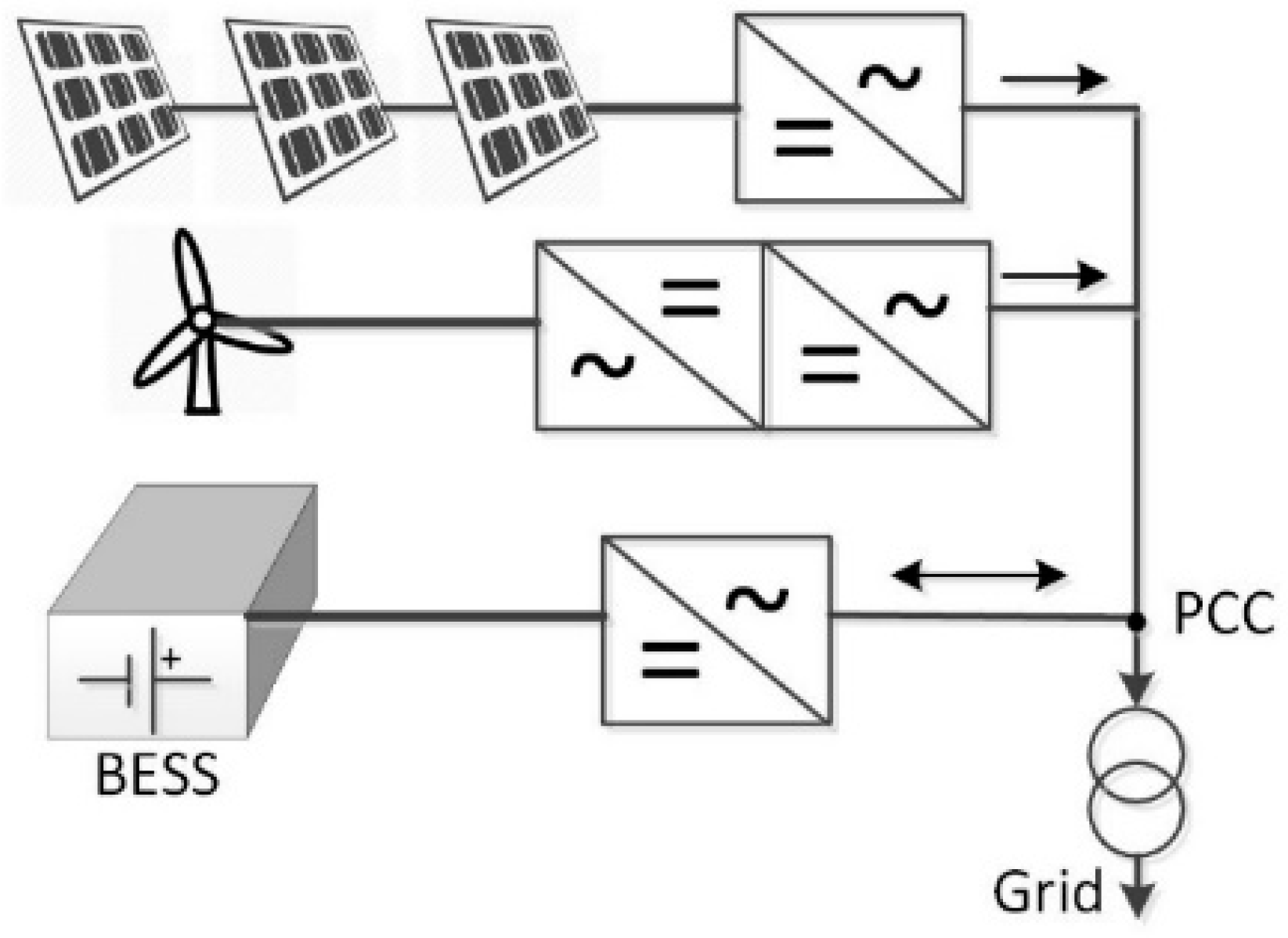
In this study, the simulated system consisted of 15 MW of PV panels, 15 MW of wind turbines, and a BESS with 10 MW of power capacity and 50 MWh of energy capacity. The solar and wind resources used are weather data from the Bureau of Meteorology [42]. The data are for Goulburn, Australia in 2001. Goulburn has a subtropical highland climate with warm summers and cold winters. Global Horizontal Irradiation (GHI) data is used as the solar resource, as PV production is highly dependent on it. Similarly, wind speed data (10-meter height) is used as the wind resource, which is scaled up to 80-meter hub height for power conversion by using the power law [43]. The wholesale prices of New South Wales were captured from Nemsight [44] in 2001 as the electricity prices in the simulation (the unit of electricity prices is AUD, due to the context of Australian electricity market. In order to keep consistency, all the costs and profits are also expressed in AUD). The box chart of electricity prices is given in Appendix A. The electricity price data for 2001 was also used to be consistent with the year of the weather data simulations.

The simulation interval in this study is 1 hour, and the optimisation process was repeated to optimise the operation of the HPP for a year. The annual operation and maintenance costs of PV, wind turbines and battery used here are 11.43 AUD and 20.33 AUD per kW [45] and 22.36 AUD per kW using a lead-acid battery [46]. Additionally, both charging and discharging efficiencies in this paper are adopted as 0.9 [22]. With similar charge and discharge patterns of battery operation in each day, the battery degradation coefficient is simplified as a constant of 0.005% per day. This assumption is consistent with the field test experiments in [47,48] with 2% capacity decrease in 1.5 years. Furthermore, the penalty rates of ${\rho }_{US}$ and ${\rho }_{OS}$ were chosen to be 1, which implies the penalty for the demanded ancillary services for undersupply and oversupply are the same with the electricity price [25]. In addition, the impacts of changing ${\rho }_{US}$ and ${\rho }_{OS}$ from 1 to 10 are investigated, which can cover the scenarios from underestimation to overestimation. When the penalty rate of ${\rho }_{US}$ equals 1, the costs from undersupply may be underestimated. In the actual power plant operation, the cost from oversupply may be partially offset by the electricity profits it makes. Therefore, the cost of oversupply will be overestimated, this is especially when the case ${\rho }_{OS}=10$.

The simulation environment is MATLAB R2016b (MathWorks, headquarters in Natick, Massachusetts, USA) with the IBM CPLEX API and the machine specification is a Dell system with an Intel i5-6200 2.30 GHz CPU and 8 GB RAM. The computational time for different strategies can be found in

Table 2. Computational times for different optimisation strategies.

Case	Computational Time for One-year Simulation
Case NB	0.26 seconds
Case DD	20.28 seconds
Case DR	211.79 seconds
Case MR	235.49 seconds

.

It is clear that Case NB without a battery installed is the fastest to be terminated out of the four strategies. It is also noticeable that Case MR only requires about 11% more computational time to have a significantly improved performance than Case DR. This is mainly due to in the implementation process. Case MR requires additional short-term forecasting in each simulation time step whereas only day-ahead forecasting is used for Case DR. The assumptions used for each simulation are summarised in

Table 3. Assumptions for the simulation modelling.

Items	Assumptions
System design	PV panels: 15 MW
	Wind turbines: 15 MW
	BESS: 10 MW of power capacity and 50 MWh of energy capacity
Battery technology	It is assumed that the degradation coefficient only changes with respect to the DOD.
	It is assumed that, with similar charge and discharge patterns of battery operation in each day, the battery degradation coefficient is simplified as a constant of 0.005% per day.
	It is assumed that a lead-acid battery will reach its lifetime when there is a capacity loss of 20%.
Market (All cost and profit values in this paper are expressed in Australian dollars (AUD).)	It is assumed that the hybrid power plant will be dispatched as a scheduled power plant.
	It is assumed that the bids from HPP are always accepted by the National Electricity Market (NEM).
	It is assumed that the penalties for oversupply and undersupply are express by the electricity prices multiplied by the penalty rates.

.

6.2. Forecasting Results

There are four different forecasting techniques that have been implemented for the prediction of both resources. The results of those techniques were compared using several metrics with persistence applied as the benchmark, mean absolute error (MAE), mean biased error (MBE), root mean square error (RMSE), normalized root mean square error (nRMSE) and the coefficient of determination ($R^2$) [48]. To make GHI and wind speed comparable, the forecasting results are normalized as per unit before calculating the errors.

Table 4. GHI and Wind Speed Forecasting Results.

Resource	Horizon	Method	MAE	MBE	RMSE	nRMSE	${\mathit{R}}^2$
GHI	D	Persistence	0.0367	1.29×10−18	0.0854	0.2537	0.9026
GHI	D	ENN	0.0394	5.8×10−4	0.0735	0.2184	0.9278
GHI	D	WNN	0.0520	0.0154	0.1000	0.2972	0.8663
GHI	D	ARIMA	0.0361	0.0016	0.0733	0.2177	0.9283
GHI	H	Persistence	0.0562	−2.78×10−6	0.0899	0.2671	0.8920
GHI	H	ENN	0.0237	−0.004	0.0441	0.1311	0.9740
GHI	H	WNN	0.0214	3.7×10−4	0.0394	0.1171	0.9792
GHI	H	ARIMA	0.0168	5.6×10−4	0.0365	0.1084	0.9822
Wind speed	D	Persistence	0.1283	−2.6×10−18	0.1708	0.5819	0.0719
Wind speed	D	ENN	0.1156	−0.0044	0.1493	0.5088	0.2903
Wind speed	D	WNN	0.1337	−0.0179	0.1748	0.5956	0.0278
Wind speed	D	ARIMA	0.1145	0.0039	0.1521	0.5184	0.2633
Wind speed	H	Persistence	0.0638	−1.27×10−19	0.0876	0.2985	0.7557
Wind speed	H	ENN	0.0651	1.7×10−4	0.0852	0.2903	0.7691
Wind speed	H	WNN	0.0677	−0.0160	0.0886	0.3020	0.7501
Wind speed	H	ARIMA	0.0657	0.00148	0.0886	0.2951	0.7614

presents a comparative summary of GHI and wind speed forecasting results using the four different methods. Note that the nomenclature, Day-ahead Forecast (D) and Hour-ahead Forecast (H), are used in Table 4 (this is also applied in Figure 5 and

Table 5. The Errors Between the Forecasted and Actual Power Generation of the HPP.

Horizon	Method	MAE	MBE	RMSE	nRMSE	${\mathit{R}}^2$
D	Persistence	3.296	0.00091	5.125	0.5134	0.5241
D	ENN	3.147	−0.7202	4.811	0.4820	0.5806
D	WNN	3.817	−0.6341	5.760	0.5770	0.3988
D	ARIMA	3.186	−0.0413	4.937	0.4946	0.5583
H	Persistence	1.974	−0.1588	3.092	0.3097	0.8268
H	ENN	1.630	−0.3909	2.696	0.2701	0.8683
H	WNN	1.666	−0.7499	2.800	0.2805	0.8580
H	ARIMA	1.580	−0.1194	2.635	0.2640	0.8742

).

Note that negative values for MBE indicate that the forecast underestimates the available resources whereas positive values indicate a tendency for undersupply. From Table 4, with the four forecasting techniques, GHI seems to be predicted with a higher accuracy than wind speed, since the MAE, MBE, RMSE and nRMSE of GHI are generally smaller than that for wind speed and the $R^2$ of GHI is also significantly larger than that for wind speed. It can also be observed that the coefficient of determination in GHI is much higher than that in wind speed. This is largely due to the predictable path of the sun, whereas there are much stronger dynamic characteristics within wind speed data. Moreover, it is noticeable that hour-ahead forecasting can significantly outperform day-ahead forecasting, except for using persistence for GHI, since hour-ahead persistence for GHI will always be tracing the previous hour’s data. This implies that the day-ahead value at the same hour is more critical than the hour-ahead value for GHI forecasting.

The nRMSE of each forecast technique is shown in Figure 5. It can be observed that it is easier for GHI to be predicted to a higher level of accuracy, as it has a more regular pattern, when using historical data, while wind speed has higher variability and is more difficult to forecast precisely by using historical data. Furthermore, hour-ahead forecasting demonstrated a much better level of accuracy than day-ahead forecasting for both resources. For most methods, hour-ahead forecasting can almost halve the forecasting errors in day-ahead forecasting. Among the four forecasting methods, ENN and ARIMA both showed good performance in terms of their accuracy and robustness. They can reduce about 20% of nRMSE on average, compared to using persistence or WNN. WNN tends to show a better performance for hour-ahead forecasting, which can achieve similar performance to ENN and ARIMA. However, for day-ahead forecasting, WNN shows worse performance, even slightly worse than persistence for both GHI and wind speed forecasting.

Furthermore, HOMER is used to transform both the forecasted and measured weather resources data to the forecasted and actual power generation, respectively. Table 5 shows the errors between the forecasted and actual power generation of the HPP predicted by HOMER. In terms of the forecasting accuracy of different forecasting methods, the performance from the errors between the forecasted and actual power generation of the HPP are generally consistent with that from the forecasting errors of GHI and wind speed. It also demonstrates the combined effect from GHI and wind speed forecasts, due to the metrics for the combined errors between the forecasted and actual power generation of the HPP, such as $R^2$, lower than that of GHI, but higher than that of wind speed. This also reflects that the forecast errors from wind speed contribute more in the forecast errors of the combined power, in comparison to that from GHI. From Table 5, we can see that ENN and ARIMA can significantly outperform the other two forecasting methods and WNN shows a poorer performance for day-ahead forecasting than persistence, but a better performance for hour-ahead forecasting.

6.3. Optimisation Results

The optimisation strategies for the battery storage were implemented with four different forecasting methods for the four cases described in Section 5.

Table 6. The Comparison of Optimisation Results when ${\rho }_{US}={\rho }_{OS}=1$ (Units: AUD).

Case	Method	Total Profit	Electricity Profit	Undersupply Cost	Oversupply Cost	O&M Cost
NB	Perfect	1,601,728	2,078,128	0	0	476,400
NB	Persistence	613,223	2,078,128	515,389	473,116	476,400
NB	ENN	666,601	2,078,128	470,079	465,048	476,400
NB	WNN	418,454	2,078,128	692,953	490,321	476,400
NB	ARIMA	675,513	2,078,128	482,102	444,113	476,400
DD	Persistence	891,222	2,042,082	264,589	186,270	700,000
DD	ENN	1,007,830	2,141,019	187,664	245,525	700,000
DD	WNN	970,804	2,287,803	304,977	312,022	700,000
DD	ARIMA	900,133	2,050,986	257,992	192,861	70,000
DR	Persistence	900,891	2,045,274	259,754	184,628	700,000
DR	ENN	1,014,593	2,143,558	184,283	244,683	700,000
DR	WNN	987,397	2,294,338	296,680	310,260	700,000
DR	ARIMA	905,935	2,053,697	255,091	192,671	70,000
MR	Persistence	1,118,056	2,077,182	117,459	141,667	700,000
MR	ENN	1,160,506	2,040,701	62,098	118,097	700,000
MR	WNN	1,174,790	2,099,715	45,016	179,910	700,000
MR	ARIMA	1,168,070	2,045,471	89,187	88,214	700,000

demonstrates the detailed optimisation results when ${\rho }_{US}={\rho }_{OS}=1$, including the total operation profits, the electricity profits, the cost from undersupply and oversupply using different forecasting techniques and battery dispatch strategies. To clarify, Case NB Perfect stands for perfect forecasting without battery.

It is noticeable that, through the comparison of results from different forecasting techniques under the same simulation case, we can justify the effectiveness of using more accurate forecast methods. Similarly, the comparison of results from different cases using the same forecasting technique can also show us the effectiveness of using more advanced dispatch strategy. For example, under Case MR, the usage of ARIMA can improve the total profit from 1,118,000 AUD using persistence to 1,168,000 AUD, an improvement of 4.5%. Moreover, when ARIMA is used as the forecasting technique, the use of mixed RHC strategy can improve the total profit from 906,000 AUD in Case DR to 1,168,000 AUD, a 28.9% improvement.

In Table 6, it is also noticeable that the electricity profits for Case NB are all the same. This is because the electricity profits rely on the actual power generation of the HPP, rather than the forecasted power generation. The actual power generation of the HPP is fixed, regardless of the forecasting techniques used. Different forecasting techniques used can still make a difference in terms of the costs from ancillary services for undersupply and oversupply.

Overall, from the perspective of using different operation strategies for dispatching the BESS, the results in Table 6 show that the overall profitability order in terms of the total operation profits can be expressed as Case MR > Case DR > Case DD > Case NB. It can be observed that the total operation profits in cases with a battery are higher than that in Case NB, where no battery is installed. Compared to Case NB, the profits of installing a battery in Case DD using persistence forecasting can increase by 45%. This illustrates the effectiveness of installing a battery in the HPP. It is also noticeable that the difference between Cases DR and DD are minimal. This is largely because both cases used the same forecasting information, i.e. the day-ahead forecasting. However, the difference between Cases DD and MR is much larger than that between Cases DR and DD. This demonstrates that the effectiveness of optimisation by integrating hour-ahead forecasting outperforms the RHC optimisation strategy for day-ahead optimisation. This further demonstrates the importance of improving the forecasting accuracy and using an advanced strategy.

For a better visualisation, Figure 6 shows the optimisation results of Cases NB, DD, DR and MR, including the total operation profits in Figure 6 (a), the profit from selling electricity in Figure 6 (b), the cost of undersupply in Figure 6 (c) and the cost of oversupply in Figure 6 (d). Note that the red horizontal lines indicate the costs/profits if we knew exactly what would happen, i.e., a perfect forecast, with no battery installed [25]. Since there are many days showing extremely high electricity prices, this may pose a huge difference when using different forecasting techniques and different optimisation strategies. Therefore, the analysis of the optimisation results will be divided into normal days (with electricity prices within 0 to 100 AUD) and extreme days (with electricity prices < 0 or > 100 AUD). Within the one-year study period, there are 346 normal days (the bars without patterns in Figure 6) and 19 extreme days (the bars with patterns in Figure 6).

Furthermore, from Figure 6(a), all simulated cases are profitable and the optimisation using the mixed RHC strategy demonstrated the highest profitability. Moreover, the smaller discrepancies of using different forecasting methods with the mixed RHC strategy also verified the effectiveness of the proposed strategy. This indicates that the usage of the proposed strategy is a useful compensation for the less favourable forecast methods. It is also clear that there are disproportionate profits from extreme days than from normal days, especially in Cases NB, DD and DR. This is largely due to the higher electricity profits, shown in Figure 6(b), from very high electricity prices during extreme days and the higher costs from ancillary services from normal days, shown in Figure 6(c) and(d).

From Figure 6(b), it is interesting to see that using the day-ahead forecasting of Cases DD and DR results in higher electricity profits than that in Case MR whereas in Figure 6(c),(d), they show the costs from ancillary services in Case MR are much lower than those in Cases DD and DR. This suggests the benefits using mixed RHC are more significant from the cost reduction than from the electricity profits increments. Moreover, the extra electricity profits from Cases DD and DR are mainly from extreme days by taking advantage of the abnormally high electricity prices, rather than from the forecast techniques or strategies.

It is also interesting to see that WNN tends to show better performance in terms of the electricity profits in Figure 6(b), which even outperforms using perfect forecasting. This largely results from arbitrage of the varying electricity prices, especially during extreme days. By comparing the bars with and without patterns in Figure 6(b), we can see the outstanding electricity profits of WNN in Figure 6(b) mainly come from the extreme days, by taking advantage of the abnormally high electricity prices. The better performance of using ENN and WNN than perfect forecasting also implied that the battery was more strongly used in extreme days to pursue higher electricity profits.

In terms of the different forecasting methods, shown with variable coloured bars in Figure 6, we can observe that ENN and ARIMA are more likely to outperform other forecasting techniques shown in Figure 6(c),but poorer when only day-ahead forecasting information is used in Cases DD and DR. This is also consistent with the forecasting results of WNN from Table 4. Moreover, in Case MR, WNN shows the lowest undersupply cost and the highest oversupply cost. This is due to its severe bias of under-prediction when using hour-ahead forecasting, which can be seen in Table 5 that WNN demonstrated the lowest negative MBE. In addition, ENN tends to have higher oversupply cost, while ARIMA tends to have higher undersupply cost. This may also explain the lower MBE of ENN than ARIMA shown in Table 5.

To further compare the performance of different optimisation strategies, the number of days when one optimisation strategy can outperform another during the whole year using the same forecasting technique are counted in

Table 7. The number of days when the case in the row outperforms that in the column using different forecasting methods.

Forecasting Methods	Cases	NB	DD	DR	MR
Persistence	NB	-	0	10	15
Persistence	DD	363	-	222	111
Persistence	DR	355	142	-	107
Persistence	MR	350	254	258	-
ENN	NB	-	0	8	2
ENN	DD	363	-	239	102
ENN	DR	357	126	-	97
ENN	MR	363	263	268	-
WNN	NB	-	1	8	3
WNN	DD	362	-	229	90
WNN	DR	357	135	-	84
WNN	MR	362	275	281	-
ARIMA	NB	-	1	6	4
ARIMA	DD	363	-	232	83
ARIMA	DR	359	133	-	82
ARIMA	MR	361	282	283	-

. For example, the first row in Table 7 indicates that there are 0, 10 and 15 days during the whole year that Case NB can outperform Cases DD, DR and MR, respectively, when persistence is applied as the forecasting technique. It is clear that the strategy in Case MR can outperform other strategies for more than 250 days. This means that the strategy of using mixed RHC strategy, combining long-term and short-term forecasts in a model predictive control framework, can overcome the deficit of forecast accuracy and provide a better overall performance for the system. The overall order in terms of the number of days when one optimisation strategy can overcome the other is Case MR > Case DD > Case DR > Case NB. Although there are more days that day-ahead optimisation can outperform day-ahead RHC strategy, day-ahead RHC strategy, with the capability of dynamic update, demonstrates a lower total cost in Table 6. This shows the optimisation process works mainly by minimising the total operation cost, rather than making the strategy outperform others with more days.

To investigate how the forecasting techniques compare against each other,

Table 8. The number of days when the method in the row outperforms that in the column in different cases.

Cases	Forecasting Methods	Persistence	ENN	WNN	ARIMA
NB	Persistence	-	170	223	174
NB	ENN	195	-	252	179
NB	WNN	142	113	-	140
NB	ARIMA	191	186	225	-
DD	Persistence	-	181	223	181
DD	ENN	184	-	248	195
DD	WNN	142	117	-	147
DD	ARIMA	184	170	218	-
DR	Persistence	-	173	225	184
DR	ENN	192	-	251	192
DR	WNN	140	114	-	144
DR	ARIMA	181	173	221	-
MR	Persistence	-	152	203	146
MR	ENN	213	-	240	177
MR	WNN	162	125	-	128
MR	ARIMA	219	188	237	-

compares the performances of forecasting methods under each specific case on a daily basis case during the whole year. For example, the first row in the table implies that there are 170, 223 and 174 days out of 365 days that persistence forecasting can outperform ENN, WNN and ARIMA, respectively, under the Case NB. From the table, it can be summarised that the order of different forecasting methods in terms of the number of days when one forecasting method can overcome the other are:

• Case NB: ARIMA > ENN > P > WNN
• Case DD: ENN > ARIMA > P > WNN
• Case DR: ENN > P > ARIMA > WNN
• Case MR: ARIMA > ENN > P > WNN

This further shows that ENN and ARIMA tend to outperform others, whereas WNN tends to show the worst performance amongst the four forecasting methods.

6.4. Impacts of Penalty Rates and Long-term Horizons

To investigate the impact of the different strategies as a function of penalty rates, the penalty rates, i.e., ${\rho }_{US}$ and ${\rho }_{OS}$, range from 1 to 10 when using ENN as the forecasting method, as from previous results it performed the best overall. Figure 7 shows the optimisation results for Cases DD, DR and MR. Note that the white plane in Figure 7 is the plane when the operation cost is zero. Overall, it is noticeable that the strategies used in Case MR, i.e. mixed RHC dispatch, can considerably outperform both in Cases DD and DR, due to using short-term forecast information to enhance the optimisation outcomes. However, the difference between Cases DD and DR are still relatively small, as we are using the same forecasting information. In fact, Case DR has a slightly lower cost, in contrast to Case DD. This comes from the effectiveness of the adoption of the RHC dispatch, which is consistent with the results in Table 6.

In addition, we can see that the impacts of changing ${\rho }_{US}$ and ${\rho }_{OS}$ in Figure 7 show the same trends, i.e. the total operation cost of the system increased gradually with the penalty rates for both undersupply and oversupply. However, for all strategies, the penalty from oversupply had a stronger influence on the cost and caused it to increase more than from undersupply at the same penalty rate. One reason for this is due to the round-trip efficiency of the battery storage, which requires slightly more charging than discharging. Besides that, this also may come from the bias of under-prediction associated with the ENN forecasting technique, which also shows in Figure 6(d) with higher cost from oversupply, in contrast to Figure 6(c) from undersupply, respectively.

As the strategy in Case MR uses a combination of long-term and short-term forecasting, it is interesting to explore how the time horizon of the long-term forecasting influence the optimisation results. Figure 8 demonstrates how the total operation profits of the hybrid system is influenced by the long-term horizons by applying the method for Case MR with long-term horizons varying from 1 to 24 hours.

When the horizon is 1 hour, the simulation results are identical to hour-ahead dispatch, which cannot be applied in a day-ahead market. In addition, when the horizon is 24 hours, it produces the same simulation as Case MR, which has a long-term horizon of 24 hours. From Figure 8(a), the subtle transitions from hour-ahead dispatch to Case MR can be observed. We can see the total operation profits are decreasing as the long-term horizon increases. This is mainly due to the decrease in forecasting accuracy as the prediction horizon extends. The use of a long-term horizon is critical to the operation of the HPP as longer forecasting provides better knowledge and reduces possible risks. However, from Figure 8, it is clear that some profit must be sacrificed when using longer-term horizons due to the inaccuracy of long-term forecasting.

It is also known from Section 6.3 that the costs from undersupply and oversupply had significant impacts on the total operation profits, which were strongly dependent on the accuracy level of the forecasting technique. Therefore, ENN and ARIMA (the pink and blue lines) in Figure 8(a) tend to outperform persistence (the black line), as the long-term horizon increases. This can be explained by its better long-term forecasting accuracy in comparison to persistence, as shown in Figure 5. However, WNN resulted in outstanding performance, despite its poor long-term forecasting accuracy. This can be explained by taking advantage of the abnormally high electricity profits shown in Figure 6(b), due to the consideration of a whole year of performance with the inclusion of extreme days. To further verify this, the performance of changing long-term horizons for normal days only are investigated, which is demonstrated in Figure 8(b). It is evident that ENN and ARIMA continue to outperform with WNN demonstrating a performance below that of persistence, due to its inaccuracy in long-term forecasting.

Moreover, it can be observed from the figures that the operation profits tend to converge when the time horizon is larger than 9 hours. This indicates that the impact from increasing the time horizon to be more than 9 hours is not as significant as that when the time horizon is smaller. When choosing the long-term time horizon for battery optimisation, on one hand, it is better to be as small as possible to ensure the forecasting accuracy. On the other hand, the time horizon needs to be large enough to take possible future scenarios into consideration. The results demonstrated in this section indicate that using around 9 hours as the long-term time horizon is the best decision to add the long-term information into the battery optimisation process. This is because this long-term time horizon can efficiently balance the trade-off between the forecasting accuracy and a broader optimisation scope. This may be affected by different sites and operation rules, which will need to be further investigated.

Dispatching the battery with 24-hour long-term scope means that all information during the whole horizon will be taken into consideration and a global optimum within the 24-hour horizon will be found. Therefore, it is highly possible that current profits are sacrificed for future events, if a high future cost has been predicted. Hence, if the long-term forecast is considered accurate enough, it will be a very valuable application in an optimisation model which combines long-term and short-term forecasting.

7. Conclusions

In this study, a mixed receding horizon control dispatch strategy to optimise BESS scheduling for the reduction of the total operation cost of a hybrid PV and wind power plant was presented. To achieve this, four forecasting methods were applied for both day-ahead and hour-ahead forecasting. We also compared the performance of different forecasting techniques used for battery optimisation.

The effectiveness of installing a battery system in a hybrid PV and wind power plant is clearly demonstrated by the simulation results, which show that an installed battery can significantly increase the total operation profit of the hybrid power plant, in this instance by at least 45%, compared to the case without a battery. In addition, there is a substantial improvement in cost optimisation with the application of the proposed mixed RHC strategy. This was implemented by integrating day-ahead and hour-ahead forecasting information with an MPC framework for the optimal operation of the BESS. The results demonstrate the success of combining long and short-term forecasting information in the proposed strategy, with an improvement of approximately 29% over the day-ahead RHC strategy. Furthermore, we have demonstrated the importance of forecasting technique accuracy, with ARIMA resulting in an improvement of 4.5% in the total profit due to increased accuracy over the persistence method. It is also worth mentioning that the proposed mixed RHC strategy alleviates poor performance due to inaccuracy in forecasted production, with less discrepancy spreading seen for the various forecasting methods used. It is important to clarify that the proposed method used can be applied to other datasets, whether it be a different hybrid system, forecasting method, timeframe or market pricing.

Another important outcome is the demonstration that by using around 9 hours as the long-term time horizon is the trade-off between a shorter time horizon, which provides more accurate forecasting results, and a broader time horizon, which considers more future predictions. Future work will focus on further investigation of the usage of a better combination of short-term and long-term forecasting techniques for battery optimisation and the impact of using different battery technologies on the optimisation results.

To conclude, the proposed strategy demonstrated significant improvement on operation profits through making full use of both short-term and long-term forecasting information. In addition, it is evident that inadequat performance from inaccurate forecasting was considerably enhanced by the optimal dispatch of the battery. However, there are also limitations in this study. In future work, the proposed methodology can be further verified by a wide range of datasets with different characteristics and improved by including the cost of battery degradation in the optimisation problem, as well as taking the potential revenue from different ancillary services markets into account.