Tuning of Controllers in Power Systems Using a Heuristic-Stochastic Approach

Abstract

A method is proposed to fit parameters of Power System Stabilizer controllers in electromechanical multimachine power systems. The use of the Non-dominated Sorting Genetic Algorithm II heuristic method and Tabu search is considered to be initial search criteria. These methods give an approximation of the values that define the controllers. Then, the stochastic approach was used to evaluate the behavior of the parameters found when considering the system’s response to the presence of random and self-sustained in-time disturbances that affect the response of the system under steady state. The stochastic approach allows the evaluation of the system’s response through the calculation of the cost of energy loss under steady state. The method is applied to two systems: a three-machine nine-busbar system, and the Interconnected System of the Greater North (Sistema Interconectado del Norte Grande) in Chile. For these systems, the proposed methodology effectively optimized the controllers and Tabu search was shown to have a better performance than the Non-dominated Sorting Genetic Algorithm II.

1. Introduction

In the operation of EPS, there are phenomena that can affect the response of the system and risk its stability due to the occurrence of disturbances that can cause oscillations with different frequencies, from which the electromechanical oscillations are the most harmful to the system. The events that can occur during the operation of the system go from sudden variations at the generation and demand level, unexpected changes in the topology of the transmission system, and events that are usually neglected, such as variations of the reference signals of the excitation systems of the machines. Those that have just been mentioned can be used to define design criteria and in that way optimize the system’s operation and evaluate the behavior of the different control elements that exist in it.

As a mechanism for solving these problems, there are different alternatives that go from the automatic generation and load disconnection schemes, devices based on power electronics at the transmission level, and the elements belonging to each generation unit, such as the controllers that act on the excitation system. In particular, PSS have been elements widely used to help a system respond to the disturbances mentioned above.

One of the main problems that exist in tuning PSS controllers is the fact that the number of parameters that define them require the search criteria to be sufficiently robust and efficient to respond to the problem associated with the dimension, i.e., determining the parameters of all the PSS needed for the adequate operation of the system in the shortest possible time.

In the specialized literature of the last five years, different valuable techniques have been reported in relation to the fitting of the parameters of the PSS controllers. In [1,2,3,4,5] a method based on neural networks is proposed to make a fitting of the controllers considering different operating conditions for the system and a dynamic response of the controller for the load conditions considered. The particular case of [2] is that it considers making a parallel fitting for the PSS and the automatic voltage regulator. In [6,7,8,9,10,11,12] models based on fuzzy logic are considered to determine an optimum fitting of the components of each controller. In [13,14] fitting strategies are proposed, respectively, for the phase compensator considering a test bench and the optimum controller of each machine according to the Heffron–Phillip model for interconnected systems. Reference [15] studies closed-loop actively controlled mechanical systems and presents some new features for experimental research in dynamics with collocated PZT ceramic sensor and actuator using a proportional-derivative controller. In [16], the collective decision optimization algorithm, a meta-heuristic based on the decision-making process of human beings, was applied for optimal design of PSSs. In [17] a control scheme based on linear matrix inequality is proposed, in order to achieve prescribed dynamic performance measures. Reference [18] presents three hybrid meta-heuristics for robust and coordinated design of PSSs. In [19] an optimal model reference adaptive system to design PSSs in multimachine EPS is described. Reference [20] proposes a new control design method in the frequency domain. It is based on the use of a modified Nyquist diagram and benefits from embedded partial pole-placement.

In [21,22], linear programming techniques are used that consider Monte Carlo simulation to validate the proposed fittings of the controllers. Robust control techniques are also widely used as reported by [23,24,25,26]. In [27], an evolutionary algorithm-based approach is shown for optimal design of PSSs for multimachine systems. The reference [28] aims to design optimal PSSs with genetic programming to improve stability through damping of the low-frequency oscillations. The work reported in [29] makes a fine fitting of the controllers’ parameters considering that there are self-sustained in-time disturbances that affect the system’s operation in steady state. The performance indicators that allow accounting for the effect that the errors in the reference signals of the excitation systems can have are defined in [29]. In such a case, it is possible to use, for example, the cost of energy loss in the permanent regime to evaluate the response of the controllers tuned by any kind of deterministic fitting method. In [29] the indicators mentioned above are calculated only for adjustment results proposed in the literature. In the present work, heuristic techniques are implemented, which are improved with the stochastic approach. The heuristic-stochastic methodology is applied to international test systems. The present work has the purpose of proposing a fitting of the PSS controllers for the Northern Interconnected Power System (SING) in Chile, considering the evaluation of the deterministic fitting from the calculation of the cost of energy loss.

The rest of this article is structured as follows: Section 2 presents a description of the problem and the mathematical model that represents an EPS as a linear system. Section 3 presents the method used to carry out the parameter tuning by means of a heuristic-stochastic approach. Section 4 contains the application to the international test systems and shows the validation of the results. Finally, Section 5 presents the conclusions.

2. Description of the Problem

The study of PSS controllers tuning in power systems is of particular interest to operators of electrical power systems. In general terms, the procedure is to obtain a linear equivalent power system based on the Lyapunov stability criterion [30]. This must be done starting from a condition of steady-state operation, established by calculating the power flow. After the equilibrium point is calculated, a linear model is determined, which properly characterizes the nonlinear dynamics of the system when dealing with small variations around the equilibrium point.

Given the linear representation of a power system, the aim of the stability study for small perturbations is to determine the eigenvalues of the system. According to the Lyapunov criterion, if the real part of all the eigenvalues is negative, the system is stable. If the real part of at least one eigenvalue is zero, the system will turn unstable as soon as any disturbance occurs during operation. Finally, if the real part of at least one eigenvalue is positive, the system will be unstable.

Considering the reasons above, it is concluded that the controller parameters allow for an improvement of system stability, i.e., with a proper adjustment of them it is possible to ensure, within certain operational limits, that the real part of all the eigenvalues of the equivalent linear system are negative.

In this context, when trying to adjust the parameters of the PSS controllers, each proposed solution will depend on the specified operating point. The main disadvantage of this is that the equilibrium point will vary for each time instant and, therefore, it is necessary to capture, somehow, the dynamics of the system in the steady state.

From what was just said, this paper proposes a methodology that allows for readjustment of the parameters obtained from deterministic techniques, whereas the dynamics around the point of steady-state operation are represented by a stochastic process. In particular, this work models and characterizes the errors in data transmission which affects the excitation systems of the machines in power systems.

As a criterion for fine adjustment of parameters, the Loss Cost in steady state is set as a performance indicator. Losses during system operation in steady state are quantified from the cost of energy and allow for the visualization of the importance of having communication and transmission systems that operate properly.

Model of the System

An electric power system is described by the following set of differential and algebraic equations:

$$\begin{array}{ccc}\hfill \dot{x}& =& f(x,y)\hfill \\ \hfill 0& =& g(x,y),\hfill \end{array}$$

(1)

where x is a vector that contains the state variables (dynamic) and y is a vector that involves the algebraic variables (voltages and angles). Functions $f\left(x\right)$ and $g\left(x\right)$ represent the system’s dynamic (of the machines) and algebraic (power flow) equations, respectively. To study small-signal stability and therefore the fitting of the controllers’ parameters, system (1) is linearized around the operation point (defined by the power flow), yielding the following equivalent linear system:

$$\begin{array}{ccc}\hfill \Delta \dot{x}& =& A\Delta x+B\Delta y\hfill \\ \hfill 0& =& C\Delta x+D\Delta y,\hfill \end{array}$$

(2)

where it is possible to determine a reduced equivalent system that is extensively used in the literature for the steady-state stability analysis and allows the making of an analysis of the oscillations from the position of the eigenvalues (in the complex plane) of matrix $A_{sys}$ [31].

$$\Delta \dot{x}=(A-B·D^{-1}·C)=A_{sys}\Delta x$$

(3)

According to [32], system (3) would have a set m of eigenvalues (where m is the number of state variables that represent the system’s machines). According to Lyapunov’s stability criterion, if each eigenvalue has the form ${\lambda }_i={\alpha }_i\pm j{\omega }_i$, then the system’s stability is ensured if and only if for every $i=1,\dots ,m$; it is true that ${\alpha }_i<0$.

As a function of the above, and considering that the position of the eigenvalues is modified by the presence of the PSS controllers, system (3) can be rewritten as follows:

$$\Delta \dot{x}=A_{sys}\left(p\right)\Delta x$$

(4)

In this case, p will be a matrix of the form $[p_1^t,\dots ,p_n^t]$, where n is the number of machines in the system and each column has the structure $p_i=[K_{PS{S}_i},T_{W_i},T_{1_i},T_{2_i},T_{3_i},T_{4_i}]$. If all the machines have controllers, then matrix p will have all its components not null.

One of the many challenges associated with parameter tuning is to determine, according to some criterion, the optimum location of the controllers. Then, it is necessary to determine which values must be taken by parameters $K_{PS{S}_i},T_{W_i},T_{1_i},T_{2_i},T_{3_i},T_{4_i}$ so that the eigenvalues of matrix $A_{sys}$ have real parts in the left complex half plane. In [29] it is stated that of all the parameters that define the controller, the gain $K_{PS{S}_i}$ is the one that affects directly the position of the real parts in the complex plane. The above notwithstanding, fitting all the controller’s parameters will be considered in the present paper.

3. Methodology for Heuristic-Stochastic Approach

Various techniques have been reported in the international literature that allow the efficient solving of the problem of the determination of the optimum parameters of PSS controllers. The reported methods make use of neural networks, fuzzy logic, robust control, and linear programming, among others.

Table 1. Summary Heuristic Techniques.

Genetic Algorithms	Tabu Search	Particle Swarm Optimization	Simulated Annealing
Based on the natural evolution and survival of the best.	Based on the prohibition of the recent.	Based on populations such as imitating how birds fly.	Based on the solidification process of solids.
A population is explored (set of solutions).	The evolution of one solution is explored at a time.	A set of particles is explored (set of solutions) in every iteration.	It is explored the neighborhood of one solution at a time.
One or multiple objectives can be used: Explain the difference between optimizing one or several objectives.
In each iteration it is generated a new population, which corresponds to the reproduction of the previous populations.	In every iteration it is evaluated the neighborhood of the actual solution, by carrying out movements in the parameters of it. without accepting prohibited movements, unless they fulfill an aspiration criterion	For every iteration it is evaluated the objective function of the particles and it is generated a new population from the velocity of the movement	In every iteration it is obtained the neighborhood of the actual solution, by carrying out movement in its parameters. There is a possibility for the solutions which do not improve their objective function.
The initial population can be random, starting from a simple technique or known solution.	The initial solution can be random, starting from a simple technique or a known solution.	The set of initial particles can be random, starting from a simple technique or a known solution	The initial solution can be random, starting from a simple technique or known answer.
The final solution can be different when using rather large populations	The final solution may vary due to Tabu time used.	The solution obtained will depend on the velocity in the movement of the particles.	The solution obtained will depend on the initial temperatures used and the cooling velocity.
Diversification and intensification techniques are considered.	There are diversification and intensification techniques based on elitism which allow us to carry out a more sophisticated search.	There is a more evolved method than the PSO, the EPSO (evolutionary particle swarm optimization), which generated new populations from mutations applied to the resulting particles in every iteration.	There are variants of the simulated annealing to improve its efficiency, such as: simulated annealing with temperature leaps or acceptation criteria with deterministic threshold.
The detention criteria used are: Having done enough iterations, reaching a designated computing time or having achieved a desired value of the objective function.
If multiple objectives are used it will be obtained a Pareto limit. It must be used a method to choose a solution of this limit.

shows a general summary of differences and potentialities of several heuristic techniques presented in the literature. These search methods are based on heuristic criteria and, therefore, finding the global optimum is not guaranteed. As a consequence, the obtained parameters correspond to a local optimum. In general, this optimum turns out to be an adequate response based on the design criteria that were previously defined. In this work, eigenvalue damping is used. This is a strong constraint for dynamic responses.

According to literature review described in Section 1, heuristic techniques have been widely used in problems that involve high-dimensional problems. In this paper, two heuristic optimization techniques are used for calibration to find optimal PSS parameters. First, the NSGA II multiobjective optimization algorithm, for several—possibly conflicting—objective functions, [33,34,35,36,37]; and second, the Tabu search algorithm, for a single associated objective.

3.1. Multiobjective NSGA II Optimization

Figure 1 shows the search algorithm used for tuning the parameters of the PSS controllers. The algorithm allows the joint tuning of all the parameters that constitute the stabilizer, and it is applied to the three above described objective functions.

From Figure 1, in (A) the maximum and minimum limits that must be assigned to the AG to tune the parameters of the PSS are established. These limits were specified from what is established in [31]. In (B) the first population of the genetic algorithm is generated, where for each of the individuals (initial solutions) the power flow is ran (equilibrium point), and then in (D) the system is linearized to get the eigenvalues of the EPS. In this way, the aptitude of each individual is evaluated by means of the objective function, until the population is finished. If the Pareto optimum is not achieved in the population, the following population is generated (following generation of individuals) in (E) and the analysis is made again from point (C). Once the Pareto optimum has been achieved, of the total number of solutions obtained, only one must be chosen for each objective function by means of some performance indicator. In the present paper, the damping of the eigenvalues has been used as a performance indicator of the EPS. First, all the dampings for each solution are calculated, and the minimum damping is chosen, and finally the solution that yields the maximum minimum damping is chosen.

The tuning methodology is based on the use of the NSGA II genetic algorithm [38]. Three objective functions are proposed that globally influence the eigenvalues of the state matrix of the linearized system. The objective functions considered are:

$$\begin{array}{ccc}\hfill F_1^{NSGA}& :& min\left(Re\left\{{\lambda }_i\right\}\right)\hfill \\ \hfill F_2^{NSGA}& :& min\left(Re\left\{{\lambda }_i({\xi }_i<0.05)\right\}\right)\hfill \\ \hfill \hspace{1em}& +& 1000·min\left(Re\left\{{({\lambda }_i({\xi }_i<0.05)+1)}^3\right\}\right)\hfill \\ \hfill F_3^{NSGA}& :& min({(-0.1-Re\left\{{\lambda }_i\right\})}^2+{(0.05-{\xi }_i)}^2)\hfill \end{array}$$

and in the three cases $i=1,\dots ,m$. For the three ${\lambda }_i$ functions it corresponds the eigenvalue i, where ${\xi }_i$ is defined as the damping of that eigenvalue.

In relation to the three proposed functions we have

• $F_1^{NSGA}:$ tries to minimize as far as possible all the real parts of the eigenvalues to ensure that all are located to the left of the imaginary axis.
• $F_2^{NSGA}:$ considers minimizing the real parts of the m eigenvalues, but this time penalizing those that have less than 5% damping by means of a cubic function displaced to $-1$ (an arbitrary choice that provides a high penalty).
• $F_3^{NSGA}:$ tries to influence the location of the real parts of the m eigenvalues as well as their damping, placing them in a region that complies with the real parts being less than $-0.1$ and the damping greater than 5%.

3.2. Tabu Search

The Tabu search is based on setting prohibitions during the search process with the purpose of avoiding the search from being trapped in a local optimum and therefore explore other regions [39]. Once the information is stored throughout the procedure on the characteristics of the visited solutions and on the operations carried out to get those solutions, the process has a memory of what has happened.

The variables that will be used to describe the algorithm are defined below:

• Sinitial: Initial solution.
• Spresent: Present solution.
• Stest: Test solution.
• BSS: Best solution of the search.
• BNS: Best neighborhood solution.

A solution is selected randomly, not affecting the final result [40], and it is stored as the best solution of the search (BSS) and present solution (Spresent). Then the test solutions (Stest) are generated, which are variations of the present solution through movements. The test solutions are evaluated in the objective function to choose the best among the test solutions, which are not Tabu or complies with an aspiration criterion, which we will call the best neighborhood solution (BNS), which is not required to be better than the present solution.

Once the BNS has been chosen, the characteristics of the movement that has been used to get to it are recorded as Tabu (for a given time). BNS is compared with BSS, and if the best neighborhood solution is better than BSS, the latter is updated with the value of BNS. Furthermore, regardless of the value obtained in BNS, it becomes the new present solution.

Finally, the short-term memory is updated, and it is verified if some stopping criterion is fulfilled. If the algorithm does not have to be stopped, the environment of the new present solution is evaluated, and the previous steps are repeated. Figure 2 illustrates the general search procedure.

To use this algorithm for tuning the PSS, the limits of the variables of the PSS parameters must be established in advance (see [31]). In each evaluation of a test solution, the system’s eigenvalues must be calculated and evaluated for every objective function. This method considers the evaluation of the following functions:

$$\begin{array}{ccc}\hfill F_1^{Tabu}& :& {\displaystyle min\left({\displaystyle {\displaystyle \sum _{{\alpha }_i\ge {\alpha }_0}^m}{({\alpha }_0-{\alpha }_i)}^2}\right)}\hfill \\ \hfill F_2^{Tabu}& :& {\displaystyle min\left({\displaystyle {\displaystyle \sum _{{\xi }_i\ge {\xi }_0}^m}{({\xi }_0-{\xi }_i)}^2}\right)}\hfill \\ \hfill F_3^{Tabu}& :& min\left\{\begin{array}{cc}{\alpha }_i\hfill & \mathrm{si}{\xi }_i>5\%\hfill \\ {\alpha }_i+1000·{({\xi }_i+1)}^3\hfill & \mathrm{si}{\xi }_i\le 5\%.\hfill \end{array}\right.\hfill \end{array}$$

and in the three cases we have $i=1,\dots ,m$, where m corresponds to the system’s number of eigenvalues, ${\alpha }_0$ and ${\xi }_0$ correspond to desired values of the real part and damping of the eigenvalue. The objective functions $F_1^{Tabu}$ and $F_2^{Tabu}$ were obtained from [40].

3.3. Performance of the PSS Controller in Steady State

Traditionally, the effect of the PSS controllers is evaluated when studying and analyzing the system’s response to contingencies such as short-circuits, which occur at an instant of time and are then cleared by the protection systems. However, it is interesting to consider the effect of the controller’s parameters, particularly the gain, on the deviations of the power trajectories generated in steady state.

3.3.1. Stochastic Model for Perturbation

The electric power system subjected to sustained random perturbations, of an additive nature, can be described by:

$$\Delta \dot{x}=A_{sys}\left(p\right)\Delta x+B\Delta u$$

(5)

From classical stability studies with small perturbations, it is considered that the input vector $\Delta u$ is null, and only the eigenvalues of matrix $A_{sys}$ are evaluated. In this case B is a matrix of order $Nxm$ (N: number of state variables and m: number of machines) that describes the way in which the perturbation affects the states of the system.

To evaluate PSS parameters under sustained random perturbations we will consider that there are instrumental errors in tele measuring systems which affect the reference voltage of each machine. In particular, we will suppose that for each machine:

$$\Delta V_{ref}=\Delta V_{ref}^0+{\xi }_t,$$

(6)

where:

• $\Delta V_{ref}^0$: corresponds to the situation without perturbation. Traditionally it is considered null.
• ${\xi }_t$: is the stochastic process that represents the measurement errors introduced in the excitation systems of the machines.

According to this previous description, the linear system can be described as follows:

$$\Delta \dot{x}=A_{sys}\left(p\right)\Delta x+B\Delta u\left({\xi }_t\right)$$

(7)

Considering the international literature [41,42], the Ornstein–Uhlenbeck process can be used to model random phenomena present in electric power systems.

In this context, it is considered that:

$$\begin{array}{ccc}\hfill {\xi }_t& =& \rho sin\left({\eta }_t\right);\rho \ge 0\hfill \\ \hfill d{\eta }_t& =& -\alpha {\eta }_{t}dt+\beta d{W}_t,\hfill \end{array}$$

where:

• $\rho$: size of perturbation
• $\alpha$ and $\beta$: are estimated from real measurements of the phenomenon that is desired to be modeled

In this particular case we have used $\alpha =1$ and $\beta =1$, as a particular case in [41].

3.3.2. Energy Loss under Steady State

The generated power deviations are transmitted one way or another into energy that is lost in the system, since they correspond to power variations over the consignments that the machines must inject during operation under permanent regime. One of the possible origins of the power deviations are found in the errors that can exist in the references of the reference signals of the excitation systems in stationary regime.

In a power system, and in particular considering at the active power deviation of a machine i caused by the presence of self-sustained in-time disturbances, the angular trajectories for different initial conditions are illustrated in Figure 3.

From what is stated in [29] and as a function of Figure 3 it is possible to define the cost of energy loss. According to what is reported in [29], the active power deviations injected by the system’s generator i are determined by:

$${\displaystyle \Delta P_{g_P}^i={\int }_{C_p^i}\Delta P_{g_i}\left(\delta \right)d{\mu }_p^i\left(\delta \right)}$$

(8)

Then, the cost of energy loss can be computed by (9):

$$\begin{array}{ccc}\hfill \mathbb{E}\left({\displaystyle \sum _{i=1}^n}{\int }_{t_0}^T\left|P_{g_P}^i(t,p,\delta )\right|dt\right)& \approx & {\displaystyle (T-t_0){\displaystyle \sum _{i=1}^n}{\int }_{C_p^i\cap [0,\infty )}\Delta P_{g_i}\left(\delta \right)d{\mu }_p^i\left(\delta \right)}\hfill \\ \hfill \hspace{1em}& +& {\displaystyle (T-t_0){\displaystyle \sum _{i=1}^n}{\int }_{C_p^i-\infty ,\cap \left[0\right)}(-\Delta P_{g_i}\left(\delta \right))d{\mu }_p^i\left(\delta \right)}\hfill \end{array}$$

(9)

where ${\mu }_p^i\left(\delta \right)$ is the invariant distribution of the power deviation generated in permanent regime [29] caused by the presence of random self-sustained in-time disturbances.

When random self-sustained in-time disturbances are introduced in the reference signals of the excitation systems, it is possible to generate power-deviation trajectories in each of the machines and in this way determine the value of the indicator of Equation (8).

3.4. The Proposed Method

This article proposes a method that aims at tuning the PSS controller parameters in two stages: first, heuristic techniques are used to find candidate parameter vectors, and then the cost of energy loss is determined for the steady state to evaluate the economic performance of the controllers. The proposed method is presented in Figure 4.

The main steps in Figure 4 can be described in detail as follows:

(A)

Simulation of power flow. As a result, an equivalent linear model is obtained for the system described in Equation (4).

(B)

Definition of variation ranges for the parameters of PSS controllers [31].

(C)

Application of a heuristic tool to adjust controller parameters.

(D)

Verification of candidate parameters for proper dynamic behavior of the system. To achieve this, three-phase short-circuits are simulated and eigenvalues are analyzed for various load conditions.

(E)

Calculation of the cost of energy losses in the steady state. This is done to evaluate performance of the candidate parameter vector when the operating point changes in time.

(F)

Evaluation of an economic criterion to be defined by the system operator. If it is not fulfilled, the process must restart.

4. Study Cases and Results

The controller fitting techniques were implemented on two multimachine systems:

4.1. Three-Machine—Nine-Busbar System

The system illustrated in Figure 5 corresponds to a typical test case reported in the international literature. The parameters used correspond to those existing in the PSAT (Power System Analysis Toolbox) simulation software.

4.1.1. Fitting of the Controller Parameters

Initially this system was equipped with three stabilizers, because no criterion was used to locate the PSS controllers in an optimum way.

To tune the PSS by Tabu search the three objective functions presented recently were used, where the values of ${\alpha }_0$ and ${\xi }_0$ used were $-0.8$ and 0.15, respectively.

Table 2. Minimum damping of the three-machine—nine-busbar IEEE system.

Function	NSGA II	Function	Tabu Search
$F_1^{NSGA}$	4.38%	$F_1^{Tabu}$	5.55%
$F_2^{NSGA}$	5.61%	$F_2^{Tabu}$	6.51%
$F_3^{NSGA}$	4.65%	$F_3^{Tabu}$	5.52%

shows the minimum damping obtained for each of the objective functions. In both search methods the $F_2^{NSGA}$ and $F_2^{Tabu}$ present greater minimum damping. Therefore, the parameters associated with those functions have been chosen as optimum solutions.

Table 2 shows that for the Tabu search the greatest minimum damping of the $F_2^{Tabu}$ function is ($6.51\%$), which is better than the ($5.61\%$) obtained from the NSGAA II algorithm with the $F_2^{NSGA}$ function. In this way we can deduce that the Tabu search yields a better result in the search for optimum parameters.

4.1.2. Optimum Location of the Controllers

With the purpose of finding a better solution than that obtained earlier, use was made of the method presented in [43], which allows selecting in an optimal way the location of the controllers. The application of this method indicates that the machines that should have a PSS are generators two and three.

In

Table 3. Minimum damping of the three-machine—nine-busbar IEEE system using Tabu search.

Function	Tabu Search
$F_1^{Tabu}$	5.48%
$F_2^{Tabu}$	6.91%
$F_3^{Tabu}$	5.69%

it is seen that the greatest minimum damping ($6.91\%$) has improved with respect to that obtained considering PSS in all the machines ($6.51\%$) and maintaining the result obtained in the F2 Tabu function.

4.1.3. Validation of the Results

Table 4. Eigenvalues associated with the electrochemical variables of the system without PSS and the three cases presented.

System without PSS		Three PSS Tabu System
Eigenvalue	$\xi$ (%)	Eigenvalue	$\xi$ (%)
$-0.19\pm j8.37$	2.28	$-0.9\pm j13.86$	6.51
$-0.72\pm j12.75$	5.64	$-1.45\pm j10.54$	13.69
Three NSGA II PSS System		Two PSS Tabu System
Eigenvalue	$\xi$ (%)	Eigenvalue	$\xi$ (%)
$-0.73\pm j13$	5.61	$-0.95\pm j13.78$	6.91
$-0.52\pm j8.67$	6.09	$-1.16\pm j9.66$	11.93

presents the eigenvalues associated with the electromechanical modes, with their respective dampings. It is seen that the tuning using the Tabu search, starting from the $F_2^{Tabu}$ function, gives better results. It should be mentioned that for this system the electromechanical modes are those that present the least damping, so the other eigenvalues have better damping, guaranteeing the system’s total stability.

To validate the fittings of the parameters of the controllers, the system’s dynamic response was analyzed when three-phase faults were applied to busbars 4 and 7.

Figure 6 shows the trajectory of the velocity of machine 1 when a three-phase short-circuit occurs at busbar 4. The velocity curves are shown considering the following cases: without PSS, three PSS (NSGA II), three PSS (Tabu), and two PSS (Tabu), with the best solution corresponding to the latter case.

Figure 7 the same analysis as the one presented above is made, but this time considering the occurrence of a three-phase fault at busbar 7. Similarly, we see that the best response of the three-machine system is obtained when there are two PSS tuned from a Tabu search.

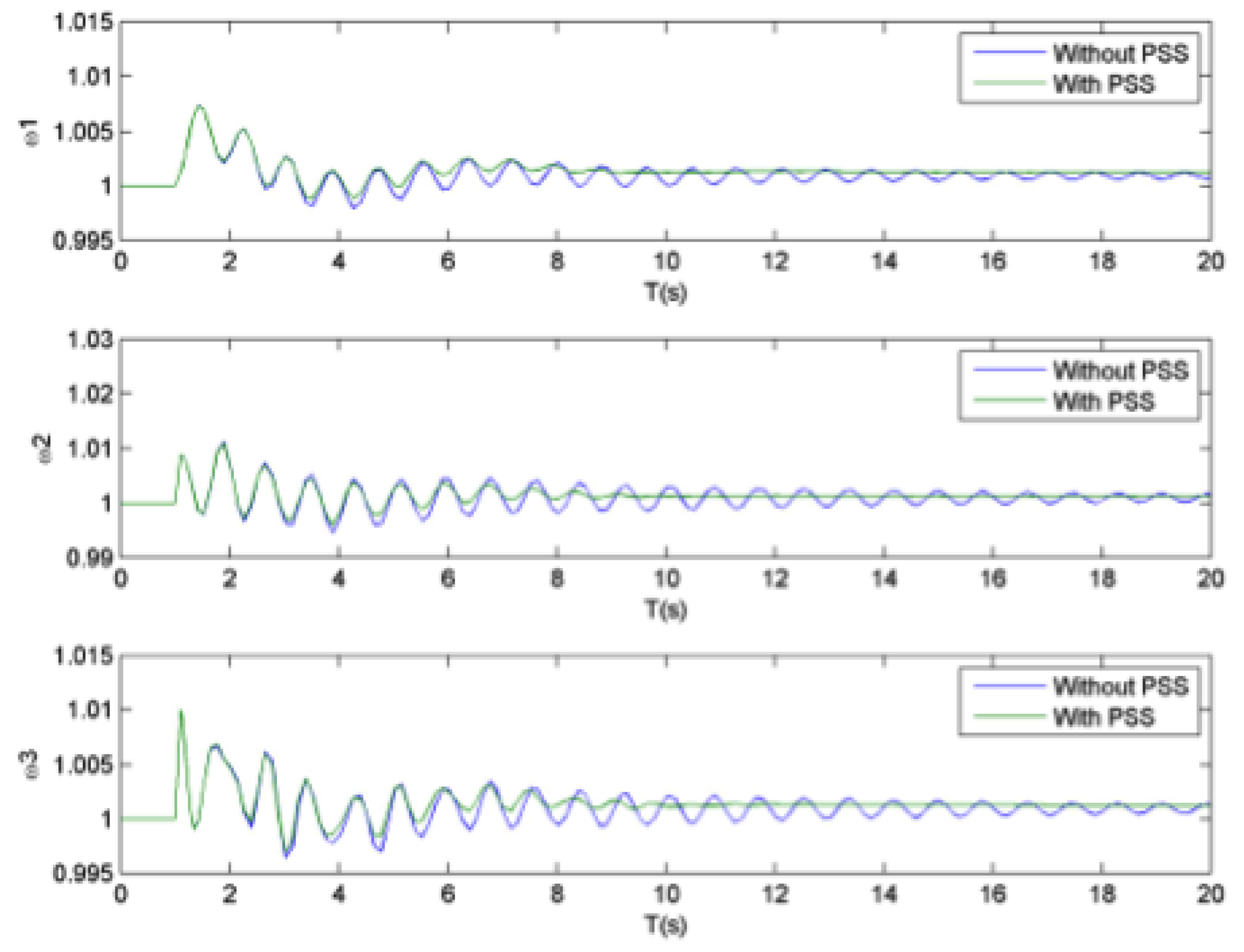
Figure 8 presents the velocity response of machines 1, 2, and 3 to a three-phase fault at busbar 4, considering the system with and without PSS (located in machines 2 and 3 after the fitting by Tabu search). It is seen that the oscillations in steady state are reduced in the presence of the two defined controllers.

Furthermore, and with the purpose of validating at the systemic level the parameters obtained from the Tabu search, Figure 9 shows the velocity response of machines 1, 2, and 3 to a three-phase fault at busbar 7.

4.2. Chilean Northern Interconnected Power System (Sing)

The Northern Interconnected Power System is one of the two main electric systems in Chile. At present, it is in constant growth due to the incorporation of new generation means, in particular non-conventional renewable energy sources. Figure 10 is a schematic diagram.

In this case, we used a reduced system of the SING, represented in Figure 11, with the parameters obtained from the reports of the system’s operator. This EPS is equipped with five power stabilizers located in machines 5, 6, 8, 9, and 16. Although these ensure the system’s stability, the aim is to improve the damping of the oscillations, including PSS controllers where required. Twenty-two power stabilizers were placed using the participation factor method [43], and they were tuned by Tabu search. According to this approach, only machine 6 was equipped without a PSS.

4.2.1. Optimum Location and Fitting of the Controllers’ Parameters

In the tuning process by Tabu search use was made of the three objective functions presented earlier, where the values used for ${\alpha }_0$ and ${\xi }_0$ are −0.8 and 0.15, respectively. In the refitting process of the system’s parameters, the three functions improve the stability after small system disturbances, achieving the required 5%.

Table 5. Minimum damping of the SING with Tabu search.

Function	Tabu Search
$F_1^{Tabu}$	5.31%
$F_2^{Tabu}$	6.12%
$F_3^{Tabu}$	6.09%

shows the system’s minimum damping, where the $F_2^{Tabu}$ function presents a greater minimum damping.

4.2.2. Validation of Results

The system’s eigenvalues and the effect of the power stabilizers in the time domain are presented after a balanced three-phase fault occurs at busbar 33. Because of the large number of eigenvalues that this real system has, only the eigenvalues associated with the electromechanical modes are presented, which are those that have the least damping.

Table 6. Eigenvalues associated with the electromechanical variables of the SING.

SING with 5 PSS		SING with 22 PSS
Eigenvalue	$\xi$ (%)	Eigenvalue	$\xi$ (%)
$-0.31\pm 9.1j$	3.44	$-0.9\pm 14.75j$	6.12
$-0.28\pm 6.84j$	4.1	$-1.16\pm 18.64j$	6.24
$-0.49\pm 9.19j$	5.35	$-1.64\pm 11.61j$	13.97
$-0.9\pm 14.67j$	6.1	$-1.63\pm 11.53j$	13.98
$-1.16\pm 18.64j$	6.24	$-1.92\pm 12.79j$	14.82
$-0.56\pm 8.55j$	6.49	$-1.2\pm 7.97j$	14.88
$-0.49\pm 7.41j$	6.64	$-1.41\pm 9.37j$	14.89
$-0.55\pm 6.74j$	8.17	$-0.85\pm 5.66j$	14.89
$-0.63\pm 7.6j$	8.2	$-1.01\pm 6.71j$	14.9
$-0.54\pm 6.3j$	8.56	$-1.22\pm 8.05j$	14.92
$-0.74\pm 7.68j$	9.56	$-1.03\pm 6.86j$	14.93
$-0.58\pm 5.43j$	10.63	$-0.98\pm 6.48j$	14.95
$-0.61\pm 5.59j$	10.91	$-1.12\pm 7.39j$	15.03
$-0.75\pm 6.42j$	11.62	$-1.17\pm 7.73j$	15.04
$-0.9\pm 7.58j$	11.78	$-1.04\pm 6.8j$	15.06
$-0.93\pm 6.81j$	13.47	$-1.41\pm 9.21j$	15.15
$-1.53\pm 9.33j$	16.16	$-0.89\pm 5.78j$	15.24
$-0.62\pm 3.79j$	16.16	$-1.08\pm 6.91j$	15.45
$-1.71\pm 9.91j$	17.01	$-1.3\pm 7.6j$	16.82
$-1.45\pm 8.4j$	17.05	$-1.22\pm 6.94j$	17.39
$-4.95\pm 12.4j$	37.07	$-3.4\pm 13.49j$	24.47
$-6.61\pm 9.85j$	55.72	$-6.7\pm 10.04j$	55.51

shows that two of the eigenvalues of the base system, associated with the electromechanical modes (only 5 PSS), do not have a damping greater than 5%. But in the case in which 22 PSS are used the damping goes from 3.44% to 6.12%, improving the indicator by 2.88%.

To see the effects of the added PSS and validate the results shown above, Figure 12 presents the response of the angular velocity of machines 1, 7, and 10 after a three-phase fault occurs at bar 33.

According to Figure 12, the system’s response with the 22 controllers is slightly better than when there are only 5 PSS.

4.3. Analysis of the Real Part Close to the Origin under Different Load Conditions

In this section, the three-machine—nine-busbar system and the Interconnected System of the Greater North are subjected to light, nominal, and heavy loading conditions. In this validation test, we determine eigenvalues and identify those closest to the origin.

From

Table 7. Real part closest to the origin.

System	Light Loading	Nominal Loading	Heavy Loading
Three-machine—nine-bus	$-0.0987$	$-0.0988$	$-0.0988$
SING	$-0.0749$	$-0.0745$	$-0.0741$

we can guarantee that the real parts of the new solutions are in the neighborhood of the values obtained in the nominal loading, so the stability is not affected. This assertion is important for the system operator considering that PSSs will have a better response under different conditions.

In addition, Figure 13 and Figure 14 show eigenvalues considering proposed solutions respect to the situation without PSS. In all cases presented—light, nominal, and heavy loading—both systems improve stability.

4.4. Performance of the PSS Controller in Steady State

For the SING, we have assumed that in all the system’s machines there are errors in the excitation signals such that the range over which those disturbances can oscillate is $\pm 8\%$. The model used to represent the self-sustained variations in permanent regime correspond to the process called Ornstein–Uhlenbeck (which was fitted as reported in [29]).

As a function of the above, the average cost of energy loss for every machine, for the parameters obtained from the Tabu search algorithm, is shown in

Table 8. Cost of energy loss under permanent regime for each machine (in 10,000 dollars per year).

Disturbance ($\mathit{\rho }$)	SING with 5 PSS	SING with 22 PSS
0	0.0003	0.0003
0.02	0.4860	0.5037
0.04	0.9720	1.0074
0.06	1.4579	1.5111
0.08	1.9439	2.0148

:

Notice that according to what is indicated in Table 8, when the size of the disturbance is null, i.e., $\rho =0$, there is no great difference if the SING has 5 or 22 PSS controllers. As the size of the disturbance increases ($\rho \ne 0$), the cost of losses also increases. In the case in which the SING has 22 PSS, the average cost per machine increases 3.5% with respect to the original case (only 5 PSS).

From the traditional standpoint, where only dynamic events that occur at a single time instant are considered, we have shown that the dynamics of the SING improves substantially when 22 controllers instead of only five are considered. However, it is also interesting to note that with the estimation of the cost of energy loss in permanent regime the same conclusion is not necessarily reached. Therefore, in addition to considering as a design criterion of the PSS the proper response of the system to step-type events, it is also necessary to include the system’s behavior (including the controllers) in the permanent regime operation.

5. Conclusions

A method has been presented for tuning PSS controllers in multimachine systems, considering heuristic tools and validating the results obtained from static and dynamic simulations, thus succeeding in damping the system’s oscillatory modes.

It is verified that the Tabu search yields better results than the NSGA II algorithm, and this was shown on the international three-machine—nine-busbar system, in addition to the simulations made on Chile’s SING system.

In relation to the damping of the oscillatory modes of the system equivalent to the SING, improvements were achieved using PSS optimally localized and tuned with the Tabu search heuristic. Using this method, the damping of the oscillations associated with electromechanical modes was improved significantly, reaching the 5% required by the Chilean network standards.

Finally, it is proposed to include the cost of energy loss in permanent regime as a performance indicator of the PSS. This index allows the complementation of the traditional search methods that only include the analysis of the system’s response to dynamic events that occur in a single instant of time.

References

- Kamalasadan, S.; Swann, G.; Yousefian, R. A Novel System-Centric Intelligent Adaptive Control Architecture for Power System Stabilizer Based on Adaptive Neural Networks. Syst. J. IEEE 2014, 8, 1074–1085. [Google Scholar] [CrossRef]
- Farahani, M. A Multi-Objective Power System Stabilizer. Power Syst. IEEE Trans. 2013, 28, 2700–2707. [Google Scholar] [CrossRef]
- Cheng, L.; Chen, G.; Gao, W.; Zhang, F.; Li, G. Adaptive Time Delay Compensator (ATDC) Design for Wide-Area Power System Stabilizer. Smart Grid IEEE Trans. 2014, 5, 2957–2966. [Google Scholar] [CrossRef]
- Suo, M.; Li, Y.; Huang, G. Multicriteria decision making under uncertainty: An advanced ordered weighted averaging operator for planning electric power systems. Eng. Appl. Artif. Intell. 2012, 25, 72–81. [Google Scholar] [CrossRef]
- Halilčević, S.S.; Gubina, F.; Gubina, A.F. The composite fuzzy reliability index of power systems. Eng. Appl. Artif. Intell. 2011, 24, 1026–1034. [Google Scholar] [CrossRef]
- Nogueira, F.; Barra, W.; da Costa, C.; de Moraes, A.; Gomes, M.; de Lana, J. Design and experimental evaluation tests of a Takagi—Sugeno power system stabiliser. Gener. Transm. Distrib. IET 2014, 8, 451–462. [Google Scholar] [CrossRef]
- Vakula, V.; Sudha, K. Design of differential evolution algorithm-based robust fuzzy logic power system stabiliser using minimum rule base. Gener. Transm. Distrib. IET 2012, 6, 121–132. [Google Scholar] [CrossRef]
- Khan, M.W.; Choudhry, M.A.; Zeeshan, M.; Ali, A. Adaptive fuzzy multivariable controller design based on genetic algorithm for an air handling unit. Energy 2015, 81, 477–488. [Google Scholar] [CrossRef]
- Smoczek, J. Experimental verification of a GPC-LPV method with {RLS} and P1-TS fuzzy-based estimation for limiting the transient and residual vibration of a crane system. Mech. Syst. Signal Process. 2015, 62–63, 324–340. [Google Scholar] [CrossRef]
- Lei, Y.; He, Z.; Zi, Y.; Hu, Q. Fault diagnosis of rotating machinery based on multiple {ANFIS} combination with {GAs}. Mech. Syst. Signal Process. 2007, 21, 2280–2294. [Google Scholar] [CrossRef]
- Ray, P.K.; Paital, S.R.; Mohanty, A.; Eddy, F.Y.; Gooi, H.B. A robust power system stabilizer for enhancement of stability in power system using adaptive fuzzy sliding mode control. Appl. Soft Comput. 2018, 73, 471–481. [Google Scholar] [CrossRef]
- Bouchama, Z.; Essounbouli, N.; Harmas, M.; Hamzaoui, A.; Saoudi, K. Reaching phase free adaptive fuzzy synergetic power system stabilizer. Int. J. Electr. Power Energy Syst. 2016, 77, 43–49. [Google Scholar] [CrossRef]
- De Marco, F.; Martins, N.; Rezende Ferraz, J. An automatic method for power system stabilizers phase compensation design. Power Syst. IEEE Trans. 2013, 28, 997–1007. [Google Scholar] [CrossRef]
- Gurrala, G.; Sen, I. Power System Stabilizers Design for Interconnected Power Systems. Power Syst. IEEE Trans. 2010, 25, 1042–1051. [Google Scholar] [CrossRef]
- Horodinca, M. A study on actuation power flow produced in an active damping system. Mech. Syst. Signal Process. 2013, 39, 297–315. [Google Scholar] [CrossRef]
- Dey, P.; Bhattacharya, A.; Das, P. Tuning of power system stabilizer for small signal stability improvement of interconnected power system. Appl. Comput. Inf. 2017. [Google Scholar] [CrossRef]
- Soliman, H.M.; Yousef, H.A. Saturated robust power system stabilizers. Int. J. Electr. Power Energy Syst. 2015, 73, 608–614. [Google Scholar] [CrossRef]
- Peres, W.; Júnior, I.C.S.; Filho, J.A.P. Gradient based hybrid metaheuristics for robust tuning of power system stabilizers. Int. J. Electr. Power Energy Syst. 2018, 95, 47–72. [Google Scholar] [CrossRef]
- Hemmati, R. Power system stabilizer design based on optimal model reference adaptive system. Ain Shams Eng. J. 2018, 9, 311–318. [Google Scholar] [CrossRef]
- Gomes, S.; Guimarães, C.; Martins, N.; Taranto, G. Damped Nyquist Plot for a pole placement design of power system stabilizers. Electr. Power Syst. Res. 2018, 158, 158–169. [Google Scholar] [CrossRef]
- Jabr, R.; Pal, B.; Martins, N. A Sequential Conic Programming Approach for the Coordinated and Robust Design of Power System Stabilizers. Power Syst. IEEE Trans. 2010, 25, 1627–1637. [Google Scholar] [CrossRef]
- Sebaa, K.; Gueguen, H.; Boudour, M. Mixed integer non-linear programming via the cross-entropy approach for power system stabilisers location and tuning. Gener. Transm. Distrib. IET 2010, 4, 928–939. [Google Scholar] [CrossRef]
- Surinkaew, T.; Ngamroo, I. Coordinated Robust Control of DFIG Wind Turbine and PSS for Stabilization of Power Oscillations Considering System Uncertainties. Sustain. Energy IEEE Trans. 2014, 5, 823–833. [Google Scholar] [CrossRef]
- Dill, G.; e Silva, A. Robust Design of Power System Controllers Based on Optimization of Pseudospectral Functions. Power Syst. IEEE Trans. 2013, 28, 1756–1765. [Google Scholar] [CrossRef]
- Jabr, R.; Pal, B.; Martins, N.; Ferraz, J. Robust and coordinated tuning of power system stabiliser gains using sequential linear programming. Gener. Transm. Distrib. IET 2010, 4, 893–904. [Google Scholar] [CrossRef]
- Simfukwe, D.; Pal, B.; Jabr, R.; Martins, N. Robust and low-order design of flexible ac transmission systems and power system stabilisers for oscillation damping. Gener. Transm. Distrib. IET 2012, 6, 445–452. [Google Scholar] [CrossRef]
- Derafshian, M.; Amjady, N. Optimal design of power system stabilizer for power systems including doubly fed induction generator wind turbines. Energy 2015, 84, 1–14. [Google Scholar] [CrossRef]
- Shafiullah, M.; Rana, M.J.; Alam, M.S.; Abido, M. Online tuning of power system stabilizer employing genetic programming for stability enhancement. J. Electr. Syst. Inf. Technol. 2018, 5, 287–299. [Google Scholar] [CrossRef]
- Verdejo, H.; Vargas, L.; Kliemann, W. Improving power system stabilisers performance under sustained random perturbations. Gener. Transm. Distrib. IET 2012, 6, 853–862. [Google Scholar] [CrossRef]
- Colonius, F.; Kliemann, W. The Dynamics of Control; Birkhauser: Basel, Switzerland, 2000. [Google Scholar]
- Sauer, P.; Pai, A. Power System Dynamics and Stability; Stipes Publishing LLC.: Champaign, IL, USA, 2006. [Google Scholar]
- Rogers, G. Power System Oscillations; Power Electronics and Power Systems; Springer: New York, NY, USA, 1999. [Google Scholar]
- Li, F.F.; Qiu, J. Multi-objective optimization for integrated hydro–photovoltaic power system. Appl. Energy 2016, 167, 377–384. [Google Scholar] [CrossRef]
- Ghazvini, M.A.F.; Soares, J.; Horta, N.; Neves, R.; Castro, R.; Vale, Z. A multi-objective model for scheduling of short-term incentive-based demand response programs offered by electricity retailers. Appl. Energy 2015, 151, 102–118. [Google Scholar] [CrossRef]
- Hu, Y.; Bie, Z.; Ding, T.; Lin, Y. An NSGA-II based multi-objective optimization for combined gas and electricity network expansion planning. Appl. Energy 2016, 167, 280–293. [Google Scholar] [CrossRef] [Green Version]
- Arora, R.; Kaushik, S.; Arora, R. Multi-objective and multi-parameter optimization of two-stage thermoelectric generator in electrically series and parallel configurations through NSGA-II. Energy 2015, 91, 242–254. [Google Scholar] [CrossRef]
- Boyaghchi, F.A.; Molaie, H. Advanced exergy and environmental analyses and multi objective optimization of a real combined cycle power plant with supplementary firing using evolutionary algorithm. Energy 2015, 93, 2267–2279. [Google Scholar] [CrossRef]
- Deb, K.; Pratap, A.; Agarwal, S.; Meyarivan, T. A fast and elitist multiobjective genetic algorithm: NSGA-II. Evol. Comput. IEEE Trans. 2002, 6, 182–197. [Google Scholar] [CrossRef] [Green Version]
- Glover, F.; Laguna, M. Tabu Search; Kluwer Academic Publishers: Norwell, MA, USA, 1997. [Google Scholar]
- Abido, M.; Abdel-Magid, Y. Robust design of multimachine power system stabilisers using tabu search algorithm. Gener. Transm. Distrib. IEE Proc. 2000, 147, 387–394. [Google Scholar] [CrossRef]
- Loparo, K.; Blankenship, G. A probabilistic mechanism for small disturbance instabilities in electric power systems. IEEE Trans. Circuits Syst. 1985, 32, 177–184. [Google Scholar] [CrossRef]
- Perninge, M.; Knazkins, V.; Amelin, M.; Söder, L. Modeling the electric power consumption in a multi-area system. Eur. Trans. Electr. Power 2011, 21, 413–423. [Google Scholar] [CrossRef]
- Hsu, Y.Y.; Chen, C.L. Identification of optimum location for stabiliser applications using participation factors. Gener. Transm. Distrib. IEE Proc. C 1987, 134, 238–244. [Google Scholar] [CrossRef]
Figure 1.
Search algorithm of the PSS parameters. NSGA II method.
Figure 2.
Search algorithm of the PSS parameters. Tabu search method.
Figure 3.
Active power deviations and their respective ranges in permanent regime.
Figure 4.
Proposed Method for heuristic-stochastic approach.