Hybrid Model for Determining Dual String Gas Lift Split Factor in Oil Producers


Department of Petroleum Engineering, Faculty of Engineering, Universiti Teknologi PETRONAS, Seri Iskandar 32610, Perak Darul Ridzuan, Malaysia
*
Authors to whom correspondence should be addressed.
Energies 2019, 12(12), 2284; https://doi.org/10.3390/en12122284
Submission received: 22 March 2019
/
Revised: 15 April 2019
/
Accepted: 15 April 2019
/
Published: 14 June 2019
(This article belongs to the Special Issue Sustainability of Fossil Fuels)
Abstract
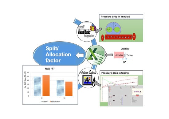
:Upstream oil production using dual string completion, i.e., two tubing inside a well casing, is common due to its cost advantage. High pressure gas is employed to lift the oil to the surface when there is insufficient reservoir energy to overcome the liquids static head in the tubing. However, gas lifting for this type of completion can be complicated. This is due to the operating condition where total gas is injected into the common annulus and then allowed to be distributed among the two strings without any surface control. High uncertainties often result from the methods used to determine the split factor—the ratio between the gas lift rate to one string over the total gas injected. A hybrid model which combined three platforms: the Visual Basics for Application programme, PROSPER (a nodal analysis tool) and Excel spreadsheet, is proposed for the estimation of the split factor. The model takes into consideration two important parameters, i.e., the lift gas pressure gradient along the annulus and the multiphase pressure drop inside the tubing to estimate the gas lift rate to the individual string and subsequently the split factor. The proposed model is able to predict the split factor to within 2% to 7% accuracy from the field measured data. Accurate knowledge of the amount of gas injected into each string leads to a more efficient use of lift gas, improving the energy efficiency of the oil productions facilities and contributing toward the sustainability of fossil fuel.
1. Introduction
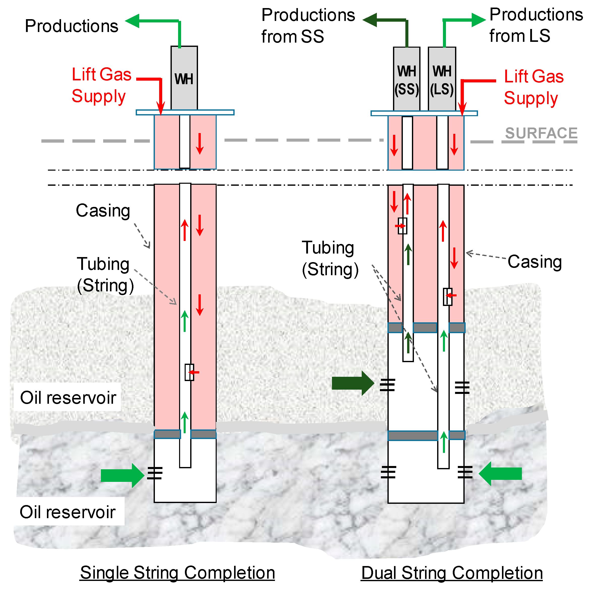
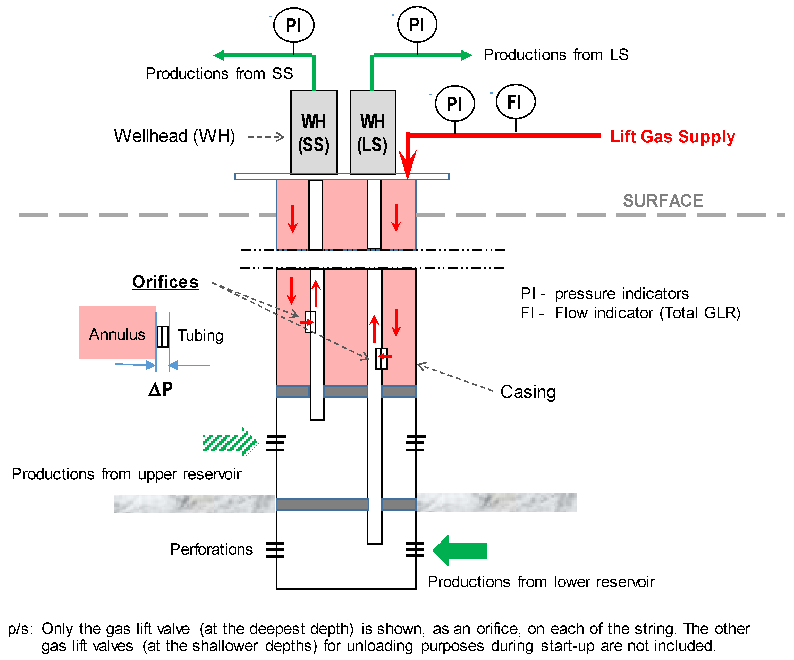
Gas lift is one of the common artificial lift techniques used in upstream oil production. It works by injecting high pressure gas into the annulus and tubing, reducing the fluids density and allowing the fluids to be produced to the surface at a lower bottom-hole pressure. Dual string completion refers to a single well casing housing two tubing, see Figure 1. The tubings are fitted into the casing side by side with all of the required accessories. Typically, the tubing will be of a different length, with one shorter than the other, to allow production from different zones. The shorter tubing is named Short String (SS), and the longer tubing is named Long String (LS) [1]. Gas lift is particularly suitable for this type of completion due to the space limitation.
The design of gas lifting for the dual string completion has proven to be a challenge. The total gas injection rate for both strings are measured at the surface, but the amount of the gas going into each tubing is difficult to determine [2]. This may lead to one of the strings getting too much gas while the other string is starved. This phenomenon is known as gas robbing. Excessive or inadequate injected gas can lead to lower well fluids production and flow instability. At the same time, it is desirable to inject the gas at the optimum level in each string to operate the gas lift system efficiently. Widianoko et al. [3] suggested placing the orifices for both LS and SS at the same depth to prevent such phenomena. This, however, may not suit the lifting requirement. There is also industry practice that simply assumes an equal split of the gas lift rate (GLIR) between LS and SS, which would hardly be the case, noting that the production behaviour may vary significantly between the two.
While the gas allocation to optimize the oil production from single string completions has been widely discussed by many researchers, the literature on gas lift optimization for dual string completion is scarce. Widianoko et al. [3] proposed the use of a trial and error technique in the field to maximize the production from the dual string well, but this is easier said than done operationally. Nishikiori et al. [4] suggested the use of a non-linear optimization method to generate the most optimum gas lift operating condition for a set of multiple single string wells. This is only applicable to a single string well where the determination of GLIR is straightforward. The optimization of the gas lift in a dual string completion would require the computation of the amount of gas going into the individual string, and the consideration of the interaction between the strings as well as with the common annulus. The split factor is defined as the ratio between the gas lift rate (GLIR) for SS and LS over the total gas lift injected. A higher split factor for a particular string means that more gas will be entering that string. This parameter is important for dual string gas lift optimization, ensuring an efficient usage of energy from the produced gas for oil production.
Eikrem et al. [5] discussed gas lift instability in a single point gas lifted dual string well using both a mathematical model and laboratory measurement. A single point gas injection for both strings does not represent a realistic field operation. In field operations, the SS gas lift injection valve was always placed shallower than that of the LS. Conejeros [6] proposed to optimize the dual string production by producing water through LS and oil through SS; his work does not consider the gas lift.
Kamis et al. [2] proposed to use the average of the GLIR for LS and SS obtained from individual well modelling. The method assumed that well tests were carried out on one string at a time while the other string is on production with the stable gas lift. The second string is to be tested immediately or as soon as possible after the first test. This is to maintain similar test conditions for both of the strings, which may not be operationally practical. The calculated gas injection rate from the single well model is matched against the surface measured test rate based on the first string’s parameters. The gasses injection rate for the second string is obtained through a simple deduction from the total gas injected. A similar approach is carried out for the second string. Consequently, each individual string will have its gas lift rate estimated, and the average of the values is then used to estimate the split factor.
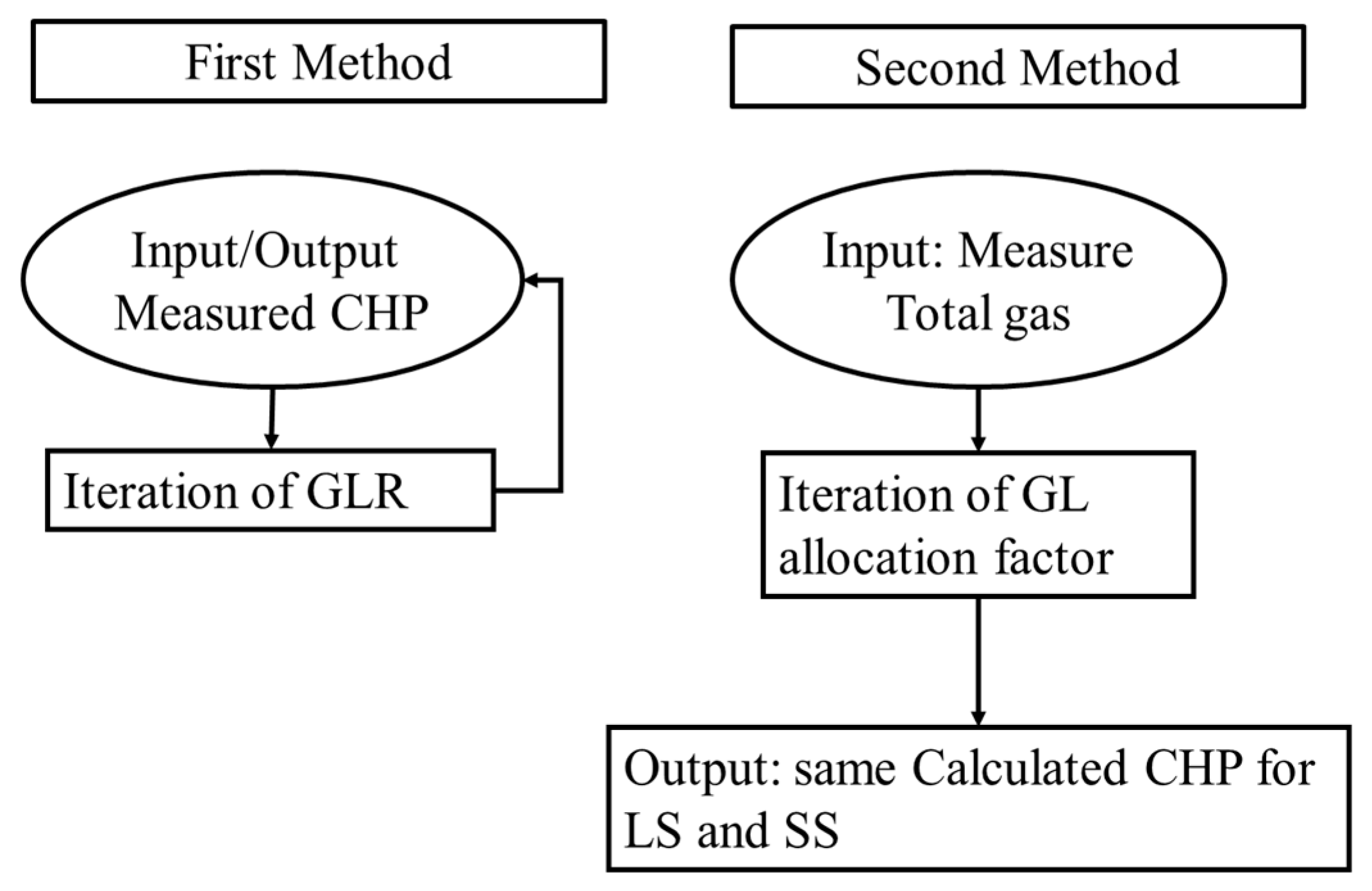
Petroleum Experts (PETEX) proposed two methods to estimate the amount of lift gas going into the LS and SS using their nodal analysis tool, PROSPER [7]. Note that PROSPER does not have the capability of modelling the dual string completion and treat the dual string completion as two separate single string completions. The first method used the measured injection or casing head pressure (CHP) to find the corresponding GLIR. The GLIR is changed, repeatedly, until the CHP estimated by the software matched the measured injection pressure. The workflow required the two strings to be solved independently. The second method uses the measured total GLIR and allocates the lift gas between the two strings assuming the same casing pressure for both of the single wells. This method reiterates the total GLIR allocation ratio as a variable, and a solution is reached when the calculated CHP is the same for both strings. The second method ensures the sum of the GLIR to the LS and SS is equal to the input of the total GLIR. Figure 2 summarises the workflow for the two methods.
Both of the two methods proposed by PETEX relied on the availability of field measured data. The solution is obtained by an iteration technique. As the software can only model a single well, the solution is obtained without considering the impact of one string on the other. The wells or the strings are considered to flow independently. The interaction of the annulus and the two strings is also ignored. The calculated casing pressure by the software is likely to be the average of the CHP at the surface, as if the LS and SS are flowing as a separate single well. The calculated CHP is almost always lower than the actual measured CHP. The estimation of the gas lift rates to the SS and LS is a mathematical exercise using the iteration technique to match a measured value. No consideration is given to the gas flow phenomenon inside the annulus and tubing.
A study by Chia et al. [8] noted that for the dual completion gas lift, as both strings share the same common annulus, it is difficult to determine the exact individual GLIR of each string. The researchers suggested to use a pre-known fix value of the gas-oil ratio (GOR) to compute the individual GLIR from the total gas measures at the surface. The assumption of a constant GOR is fallacious as the GOR value changes from time to time. It also required the well to be tested individually, which may not be practical due to operational constraints.
A few researchers have, in more recent years, proposed the use of an artificial intelligence (AI) approach to tackle gas lift optimization. Patterns of changes in operating conditions were identified through the measurement of parameters, and AI algorithms were then applied to correct the conditions. Abbasov et al. proposed a method using machine learning to attain the minimum field measured tubing head pressure oscillation, so as to achieve an optimum production. It relied mainly on field testing and no well modelling is required [9]. Xiao et al. suggested the use of a calibrated well model to establish the operating envelope for a stable production. An automated workflow is created to monitor, troubleshoot and correct the well for any instabilities during the production [10]. Both methods are only applicable to single string wells where the wells behave independently of each other.
To obtain an accurate estimate of the gas lift rates for dual string completions, the industry has to resort to a field measurement via a well tracer survey. The tracer method allows the measurement, when both strings are flowing, to account for the interaction between them. However, it is costly and operationally impractical as it requires the mobilization of expensive equipment and personnel. In addition, there is a potential production deferment related to the well work. The well tracer for the dual string can be challenging, as discussed by Abu Bakar et al. [11]. An average of six hours per survey is required with a 25% rerun for dual strings due to too many points of gas returns.
Hermank et al. proposed the use of distributed thermal sensing (DTS) and distributed acoustic sensing (DAS) for the gas lift surveillance [12]. The method is less invasive and can provide a precise injection point based on changing temperature and sound signals. However, it would require high capital investment to equip the wells with downhole optical fibers. This method will work well with the single string well but not necessarily with the dual string well. The interpretation of DTS and DAS for the dual string well is a lot more complicated given the pressure and flow dynamics within the annulus as well as between the strings and the annulus.
For an optimum production, the lift gas has to be injected at the correct rate. Excessive or inadequate injected gas can lead to a suboptimal production and flow instability [13]. So far, the various methods proposed by the researchers do not directly compute the gas lift rates to individual strings for the dual string completion. The solutions were derived by the use of an iterative approach, with simplification (such as an injection at the same depth), averaging, or equating the dual string as two separate single strings. The interactions between the lift gas inside the common annulus and the production fluids in the tubing were not taken into consideration. The results obtained can be misleading as they do not represent the actual operation of a dual string well. Little insight can be derived for gas lift troubleshooting to optimize the lift gas usage.
The objective of this study is to develop a hybrid model to determine the gas lift split factor considering the fluids flow phenomena both in the annulus and the tubing. The hybrid model will combine three platforms: the Visual Basic for Application (VBA) programme, PROSPER (a nodal analysis tool) and Excel spreadsheet to compute the gas lift rate into an individual string and subsequently the split factor. The model will be validated using a set of field measured data. This hybrid model allows for an accurate estimation of the lift gas rate for the dual string completion, enabling an efficient use of lift gas and yielding an opportunity for improving the energy efficiency of upstream production facilities.
2. Methods
The study is carried out in 3 stages:
- Development of the hybrid model for the split factor in dual string gas lift.
- Validation of the hybrid using a set of available field data
- Case study.
2.1. Modelling of Split Factor
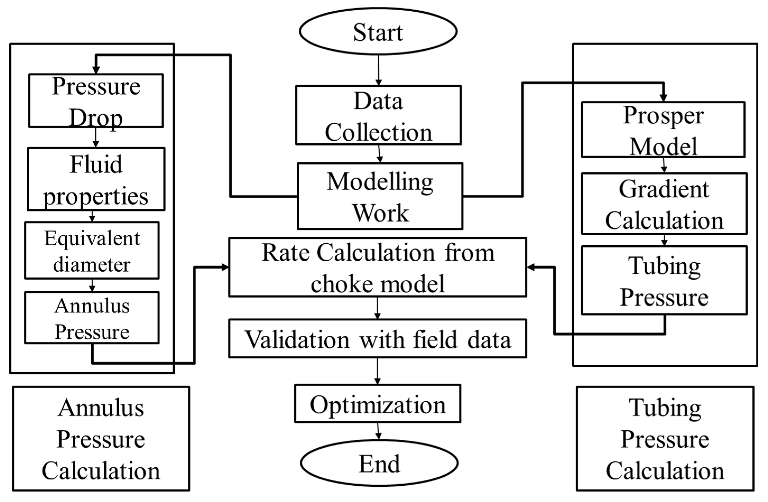
A flow chart for modelling the split factor is given in Figure 3.
The proposed model used the casing injection pressure (CHP) and total gas lift rate (GLIR) measured at the surface as the input to estimate the GLIR to both the SS and LS. Based on these individual GLIRs (estimated) and the total GLIR (measured), the split factor can be determined.
The tubing experiences pressure from the annulus (from the gas lift injection) and from the well fluid flowing from the reservoir through it. To estimate the gas lift rate, three pressure drops need to be considered (see Figure 4):
- Pressure drop in the annulus
- Pressure drop across the orifice
- Pressure drop in the tubing
The lift gas is introduced to the casing/annulus, and the pressure (CHP) is measured at the wellhead. The lift gas flowing in the annulus imposes a pressure upstream of the orifice, while the production fluid flowing inside the tubing will exert a pressure downstream of the orifice. The pressure differential across the orifice determines the amount of lift gas flowing into the tubing.
The estimation of the annulus pressure will incorporate the concept of the equivalent hydraulic diameter, which is commonly applied in a heat exchanger design to account for a non-regular flow path. PROSPER [14], a multiphase flow simulator, will be used to estimate the pressure along the tubing from the reservoir to the wellhead as the multiphase production fluids are expected to flow inside the production string from the reservoir to the wellhead. The orifice flow correlation will be used to compute the GLIR as a function of the annulus and tubing pressure difference.
2.1.1. Annulus Pressure Calculations
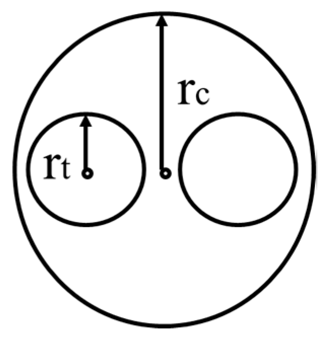
There are three pressure loss components, i.e., elevation, frictional and acceleration. ρ is the density, ν is the velocity, gc is the gravity constant, f is the friction factor and D is the flow diameter. Equation (1) is applicable for the single-phase gas flow. The considered cross-sectional flow area will be adjusted accordingly with the equivalent hydraulic diameter, to account for two concentric cylinders inside the casing (see Figure 5). The Hydraulic diameter is defined as the cross-sectional area of the channel divided by the wetted perimeter. It uses the perimeter and area to provide the diameter such that conservation of momentum is maintained. By using this term, one can handle any dimension of a flow path as one would for a round tube. The uniform flow path is expected within the annulus to the point of injection, no significant change in velocity is expected and hence the acceleration component may be ignored.
The fluid velocity V, in Equation (1), can be derived from the flowrate Q:
The equivalent hydraulic diameter, De, can be calculated using the generic equation:
From Figure 4, it can be shown that:
where rc and rt are the casing radius and tubing radius, respectively.
The Colebrook Equation, which is applicable for turbulent flow, is used to calculate the friction factor, f. The software Visual Basics for Application (VBA) is employed to handle the complicated iterations needed to solve for the friction factor, and ε is the roughness:
Re is the Reynold Numbers:
The gas properties, critical properties, Z factor and viscosity are estimated using the well-known empirical correlations. The critical temperature and pressure are required to complete the calculation for the Z factor. The Z factor is required for the calculation of the density. The viscosity is required in the calculation of the Reynolds Numbers, which is part of the solution for the friction factor calculation. The selection of the correlations used is based on accuracy and practicality.
The critical pressure Pc, and critical temperature Tc are estimated using the Sutton correlation [16] due to its simplicity for the single gas phase, requiring only the viscosity v as the input. Deckle et al. [17] recommended the use of the correlation for gas gravity under 0.75, which is compatible with the lift gas used for this study.
The Z factor is estimated using the Hall Yarborough correlation. This correlation has the highest accuracy according to the work done by Lateef in comparison to the other correlation [18]. After the Lateef modification is not significant, an original equation is used as variance in the accuracy.
The Lee, Gonzalez and Eakin [19] correlation is chosen for the viscosity estimate due to its simplicity. The accuracy does not vary much from the other correlation reported by Al-Nasser et al. [20]. The original correlation was used in comparison with one optimized by Al-Nasser et al., as the difference in accuracy is not significant.
The density is estimated as follows:
where the molecular weight of the gas, Mgas, is:
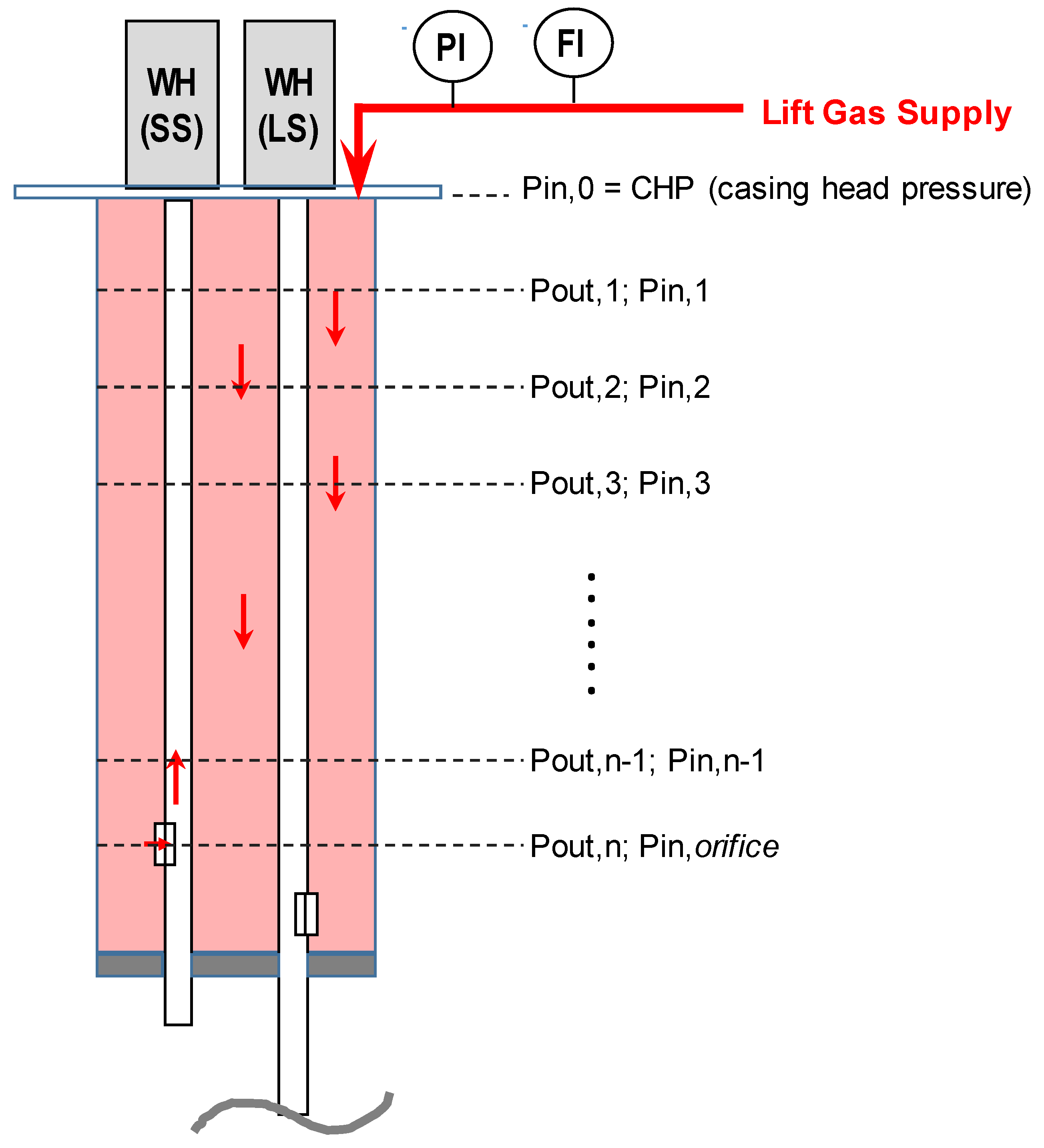
The annulus pressure along the casing length is estimated by dividing it into n, the number of node sections from the casing head to the injection point. A loop was created with VBA to iterate the pressure at the inflow, until it equals the outflow from the previous section (see Figure 6). The process continues until the pressure reaches the specified point of interest, which is the orifice valve location, the injection point. This is done to improve the resolution of the calculation and accuracy of the computation.
The composite flow path with a different inclination is created to account for the non-vertical flow direction. This is to improve the accuracy of the model. A total of 5 sections with different angles is created to mimic the flow path of the upper well section. The number of sections can be added easily for a better resolution with VBA. However, this is usually not required, as the angle would typically be low at the gas lift valve depth. The gas lift valves need to be placed at a shallow wireline accessible depth for the change-out during the well intervention, and normally this is below 60 degrees.
The temperature is assumed to follow the geothermal gradient, as a continuous gas lift under a steady state condition is expected to have achieved a thermal equilibrium. The interpolation is done to estimate the pressure at the depth, to simplify the calculation. The temperature input and output at the 5 segments is specified. In VBA, it is further broken down into n, the number of nodes, as below, similarly to the pressure for the calculation between the segments:
2.1.2. Tubing Pressure Calculations
The pressure drop required to lift the reservoir fluid to the surface at a certain rate is controlled by the wellhead choke. The pressure along the tubing is a function of the mechanical configuration, fluid properties and production rate. Several empirical and analytical correlations have been developed to estimate the pressure drop in multiphase flow depending on the reservoir and well conditions. The selection of an optimum correlation is essential to estimate the pressure drop along the tubing [21]. In this study, the multiphase flow simulator, PROSPER, will be used to calculate the pressure gradient along the inside of the tubing. The software is widely recognized for well modelling within the industry. Among the advantages are that it allows for a calibration with previous test data and that it provides a wide selection of Vertical Lift Performance (VLP) and PVT correlations.
2.1.3. Gas Lift Rate (GLIR) Calculations
The common practice in the industry is to estimate the pressure upstream of the orifice from the known lift gas gradient in the casing, and the pressure downstream of the orifice from the flowing gradient survey (FGS) in the tubing, to calculate the lift gas flow rate from the throughput chart. However, in the absence of actual fluid gradient data, usually a general gradient value (for example 0.2 psi/ft.) is assumed. This practice is more suited to a field application for a quick check. It will calculate the LS and SS individually, and does not reconcile the total gas rate or injection pressure.
In this study, the lift gas flow rate through the orifice will be calculated using the Thornhill Craver equations [22] for the orifice valve (see Equation (28)). This equation is for a compressible, one-dimensional and isentropic flow of a perfect gas through restriction; a correction factor (discharge coefficient, Cd) is added to account for deviations encountered in the real gas case [23]. The gas rate is corrected to the real condition using Equation (29), to reflect the rate at the actual down hole temperature and pressure:
where Cd is the discharge coefficient, A is the flow area (in2), P1 is the upstream pressure (psia), P2 is the downstream pressure (psia), k is the ratio of specific heat (=1.27), Fdu is the ratio of P1/P2, SG is the gas specific gravity, T is the temperature (°R), Qsc is the gas rate at the standard condition (Mscf/D) and Qinj is the gas rate at the actual condition (Mcf/D).
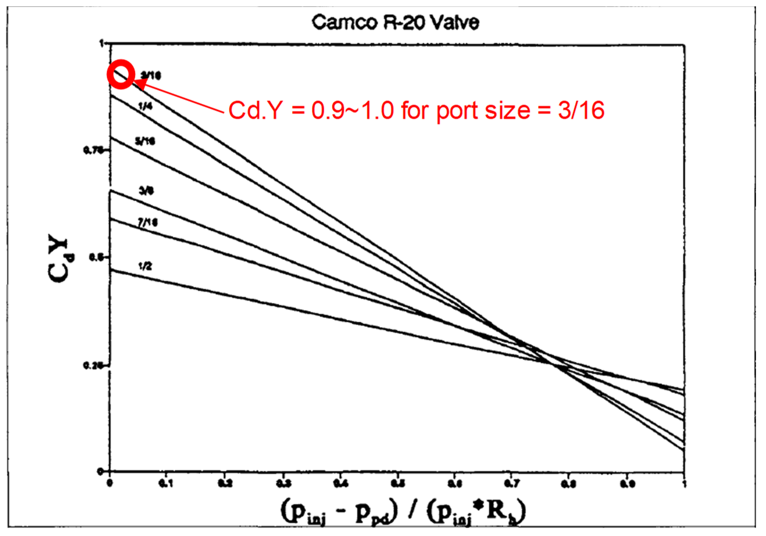
An orifice requires a more than 40% pressure drop across it to achieve a critical flow. Although a slight variation in the tubing flow regime will result in an unsteady injection rate, an orifice can accommodate a wide operation range, and it remains the most commonly used operating gas lift valve in the industry. The upstream and downstream pressure are put into Equations (28) and (29) to calculate the injection gas rate. The discharge coefficient, Cd, is taken from experimental work done by Nieberding et al. [24] (see Figure 7).
Cd is the discharged coefficient. Y, the expansion factor, equals 1 for an ideal gas at a high temperature and pressure, representative of the down-hole condition. From Figure 7, CdY is between 0.9 to 1, for the Camco R-20 with a port size equal to 3/16.
The determination of the gas lift injection assumes a steady state, continuous injection and single point injection at the SS and LS, respectively. This is representative of the gas lifted oil production whereby only the deepest gas lift valve is open during the normal operation after unloading. The valves that are installed at a shallower depth for unloading purposes are excluded, as unloading is a transient operation during the well start-up, which is to say an infrequent event.
2.2. Model Validation
The actual field data from a brown field is used to validate the proposed model. The field has a long history of gas lift application. The gas lift allocation for the dual string completion was a big problem for the field.
The field data were measured using the Well Tracer method. The method measured the concentration and travel time to allocate the amount and location of gas injected [25]. Although costly and strenuous in operation, this method provides the most accurate measured data.
2.3. Case Study
A case study was carried out to demonstrate the application of the proposed hybrid model in determining the split factor for a dual completion oil produce well “X”.
3. Results and Discussions
3.1. Annulus Pressure Calculation
The pressure calculation is conducted for the annulus via a breakdown into 5 sections, as shown in Table 1. The diameter calculated here is the equivalent hydraulic diameter. The inlet in the first section is the injection pressure, and the outlet pressure in the last section represents the choke upstream pressure. It is observed that the pressure increases from the point of the inlet down to the orifice depth, for the condition assessed, and there is an estimated increase of 42 psi that accounts for both the hydrostatic and frictional pressure differential. The number of sections is deemed sufficient as the well is vertical in the top sections, and the deviation is only observed in the last two sections.
3.2. Tubing Pressure Calculation
For this study, the best matched PVT correlations were selected. The Standing correlation is used to estimate the GOR, formation volume factor and bubble point pressure. Begg’s correlation is used for the viscosity calculation. For the VLP correlation, PE2 is selected. PE2 is an empirical correlation developed by PETEX, intended to cover a wide range of operating conditions. This correlation uses the flow map by Gould & et al., the Hagedorn Brown correlation for the slug flow and the Duns and Ros for the mist flow. In the transition regime, a combination of slug and mist results is used. It also has improved the VLP calculations for low rates and for the well stability. It provides a more accurate prediction of the minimum load-up rates [14].
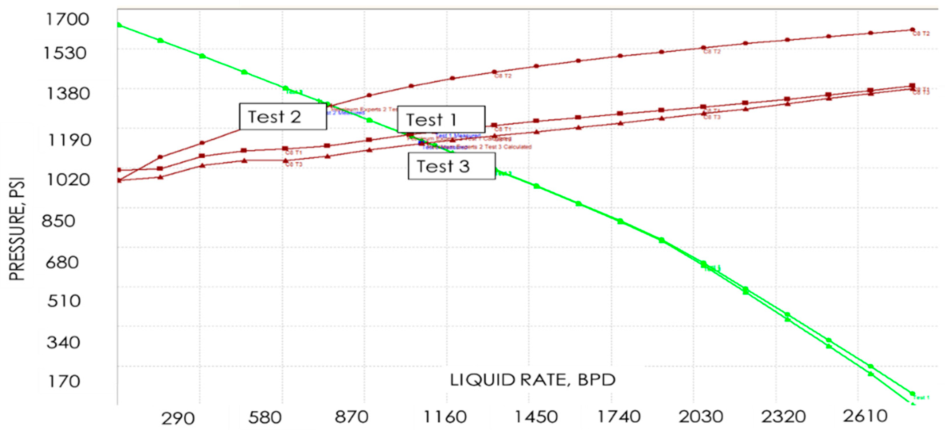
PE2 appeared to have the best match with 3 previous well tests, as shown in Figure 8. The calculated rate and flowing bottom hole pressure (FBHP) was well within the ±10% of the measured test data. It also has the lowest average absolute error compared to other vertical lift performance correlations. The inflow Performance Relationship (IPR) Model is generated with the Productivity Index (PI) model.
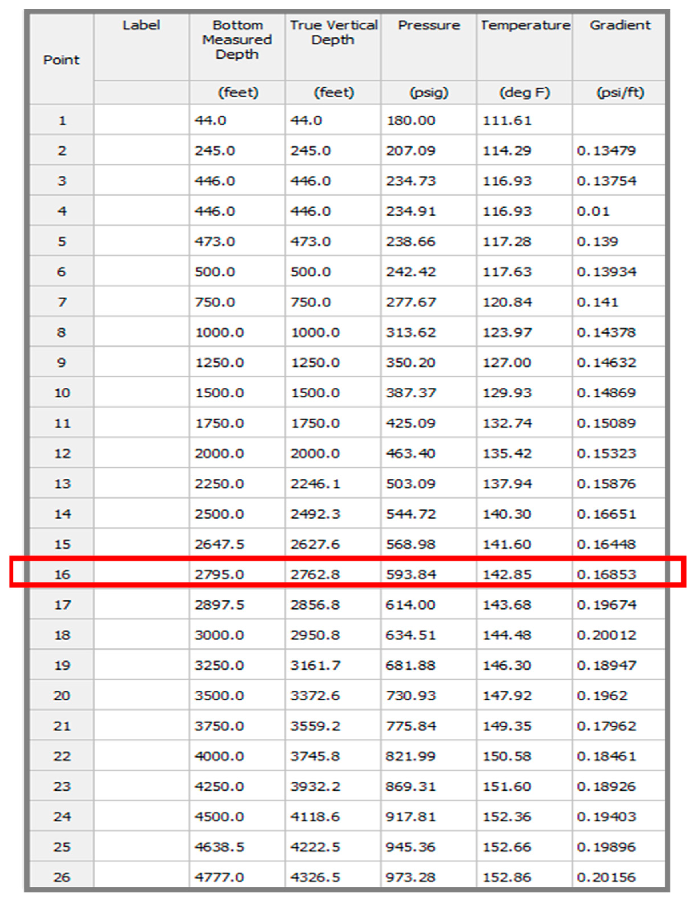
The measured parameters from the well test: the flowing tubing head pressure (FTHP), GOR, and water cut (WC), are the required input for the pressure gradient calculation. The generated pressure profile from the wellhead to the perforation depth can be seen in Figure 6. The pressure at the orifice is singled out from the depth-pressure profile to represent the downstream orifice pressure (highlighted in Figure 9).
3.3. Gas Lift Rate (GLIR) Calculation
An example of the gas lift rate calculation is given in Table 2. The GLIR is obtained via subtracting the SS injection rate from the total gas injected, assuming that all the injections from the surface go into the tubing as per the basis used by both Kamis et al. [2] and Chia et al [8]. This also provides a reconciliation to the surface measured gas rate.
3.4. Model Validaton
The split factor is calculated for the two wells, namely, wells “X” and “Y”. Both wells are dual string completion type wells, with 3½ inch production tubing and a low angle deviation angle. A wide range is observed in the measured GOR and WC for the wells. “X” SS and LS and “Y” LS are producing from the deeper reservoir, with a water breakthrough and high GOR due to depletion. “Y” SS produced from the shallower reservoir with a low water cut and is still above its bubble point, which explains the noticeable lower GOR.
A comparison between the calculated values from the model and measured date from the field is given in Table 3.
The model demonstrated that it can estimate the lift gas distributions for both well “X” and well “Y”, over a considerable range of operating conditions, to an average relative error of between 2% and 7 %, as shown in Table 3. The higher discrepancy in well “Y” is possibly due to poor matching between the well test data and the calculated PROSPER results. This could be due to inaccuracies in the measurement data collected during the well test, discrepancies in the PROSPER modelling of the actual well conditions, or both. The collected well test data were within the acceptable accuracies. For well “Y”, during the tracer survey, it was observed that multi-pointing had occurred at the LS. The PROSPER model has assumed a single injection point for LS (well “Y”). It could not mimic the multi-pointing actual conditions, hence the poor match between the measured well test data and the simulated results.
3.5. Case Studies
The proposed hybrid model is used to generate the lift gas distribution and compared to the available field well test data for well “X”, see Table 4. The field well test data were based on PETEX methods, assuming the dual strings as a single well model, as described previously in Section 1.
There is a tendency to under-allocate the lift gas for SS, overlooking gas robbing phenomena. The well test data 1 was off by 80 Mscf/D, whilst the well test data 2 was off by almost 185 Mscf/D. The calculated split ratios from the proposed hybrid model in both tests are closer to the Well Tracer measured data, indicating a higher consistency and better accuracy. This is in line with the understanding that the single well models, such as those proposed by PETEX, are limited for application due to the interaction of the gas distribution between the 2 strings.
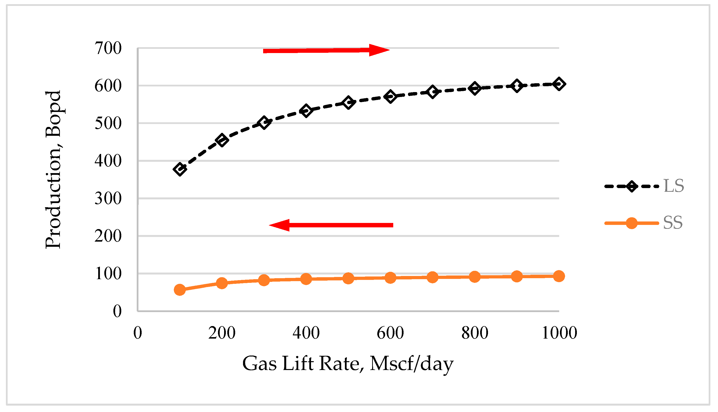
Having an accurate GLIR estimation is fundamental to the optimization of the gas lift to improve the production and hence the profitability of the well. The potential impact of an accurate GLIR estimate on the productions from well “X” can be demonstrated by Figure 10, and Table 5 and Table 6.
Figure 10 showed that the production for LS is more sensitive to gas lift rate changes. The red arrow indicates the directional changes on the GLIR redistribution for SS and LS to achieve a production optimization. Reducing the GLIR for SS by 200 Mscf/D merely cut back the production by 5 Bopd, whilst increasing the same amount will increase the production by almost 50 Bopd for LS. This is because LS is producing from a better productivity index (PI) reservoir and the water cut is also higher at 80%, resulting in the requirement for more gas to lift the total liquid. On the other hand, SS, due to a low water cut and relatively lower liquid rate, is nearing it optimum operating condition. There is an opportunity to reduce the gas lift rate for the SS and redistribute to LS to improve the production as a whole.
The variation of the production with the lift gas rate is tabulated in Table 5.
The GLIR can be varied by changing the orifice sizes. The proposed hybrid model is used to generate the split ratio between the LS and SS for the selected 3 different orifice sizes, as shown in Table 6.
The existing orifice for SS is 12/64th. By reducing the orifice size for the SS to 10/64 in. and 8/64 in., the GLIR is cut back by 128 and 262 Mscf/D respectively. This saving in the GLIR from the SS may be re-allocated to LS or other wells in the field to enhance production. An estimated 48 Bopd gain can be achieved by reducing the orifice size for the SS from 12/64 in. to 8/64 in. based on the gas lift performance curve of LS and SS.
3.6. Features, Advantages and Limitations of the Proposed Hybrid Model
The model is able to determine the lift gas rate for the individual string, via a combination usage of VBA, the available nodal analysis tool (PROSPER) and proven empirical correlations. This sets it apart from the existing practices of conducting multiple iterations to yield a mathematical solution without considering actual conditions of the dual string gas lift operation. Another advantage of the model is that it only requires surface measured parameters which can be obtained easily with high accuracy. The inputs required are the injection pressure for the casing pressure calculation and the well test parameters (GOR, FTHP, liquid rates and WC) for the tubing pressure computation. This approach provides a simplification to the calculation process.
An accurate estimate of the GLIR is fundamental to the production optimization of gas-lifted wells. This is especially crucial for dual string completion type oil producers. The application of the model for the gas lift optimization of dual string wells is demonstrated in Section 3.5., where a saving of 262 Mscf/d GLIR from SS is used to increase the production from LS by 48 Bpod. This can be extended to other dual string wells within the same field. Injecting just the right amount of gas lift for the desired production is the principle concern for operators of mature fields where the amount of gas lift available is often constrained by the existing facility system, the lift gas compressors [26]. The opportunities to enhance the production can also be realized through the optimizing of parameters such as the casing head pressure, injection depth and orifice size.
The model is developed for steady state, continuous injection conditions, which are commonly fulfilled in oil production following the unloading operations, when and where only the deepest gas lift valve is operating. It does not cater to transient operations such as those during well unloading or an unstable injection resulting from the flow instability of the production conditions. Nor does the model apply to multi-pointing, conditions whereby the lift gas enters the tubing through more than one point along the tubing. This could be due to poor design or unintentional changes in the operating condition. Under such circumstances, a transient analysis tool or field measurement may be more suitable for diagnostic purposes.
The proposed model offers a better method to quantify the gas lift split factor, thereby enabling the efficient use of gas lift, paving a way for the improvement on gas lift optimization in dual string completion and for opportunities to understand the overall produced gas usage. This would inevitably improve the energy efficiency of upstream oil production facilities.
The model can be adapted easily into the current industry gas lift optimization work flow. Lastly, the proposed hybrid model provides a potential substitute to the Well Tracer measurement method, averting the costs and risks of well intervention.
4. Conclusions
By considering the pressure drops of production fluids in tubing and the pressure gradients of the lift gas along the annulus, this proposed hybrid model enables a more accurate estimate of the gas lift split factor for dual string completion wells. In this study, the model was able to predict the split factors for well “X” and well “Y” within an accuracy of 2% and 7% from the actual measured data. This hybrid model provides far better results than the current methods, which are based on an approximation of dual strings as two separate single strings, disregarding any interactions between the strings within the same casing. An accurate knowledge of the amount of gas injected into each string leads to a more efficient use of lift gas, improving the energy efficiency in oil productions facilities and contributing toward the sustainability of fossil fuel.
Author Contributions
The idea of this research was conceptualized by all authors. K.H.C., M.Z.Z. and J.H.L. provided the guidance and supervisions; C.C.L. implemented the research, performed the analysis and wrote the paper. All authors contributed significantly to this work.
Funding
This research was funded by Yayasan Universiti Teknologi PETRONAS, YUTP-FRG research grant 015LC0-009.
Conflicts of Interest
The authors declare no conflict of interest.
Abbreviations
The following abbreviations are used in this manuscript.
| CHP | Casing Head Pressure |
| FGOR | Free Gas Oil Ratio |
| FTHP | Flowing Tubing Head Pressure |
| GLIR | Gas Lift Rate |
| GOR | Gas Oil Ratio |
| LS | Long String |
| PFD | Process Flow Diagram |
| PI | Productivity Index |
| PVT | Pressure, Temperature and Volume |
| SS | Short String |
| SGOR | Solution Gas Oil Ratio |
| VBA | Visual Basic Application |
| WC | Water Cut |
| Angle from the horizon, degree | |
| Z | Compressibility factor |
| Tc | Critical Temperature, °R |
| Pc | Critical Pressure, psia |
| P | Density, lb/ft3 |
| D | Diameter, inches |
| Cd | Discharge Coefficient |
| P2 | Downstream pressure, psia |
| De | Equivalent hydraulic diameter, inches |
| A | Flow area, in2 |
| f | Friction factor |
| gc | Gravity constant |
| Qsc | Gas rate at standard condition, Mscf/D |
| Qinj | Gas Rate at actual condition, Mscf/D |
| L | Length, ft |
| M | Molecular weight, lbmol |
| N | Number of nodes |
| P | Pressure, psia |
| Tpr | Pseudo reduced Temperature |
| Ppr | Pseudo reduced Pressure |
| rc | Radius of tubing, in |
| rt | Radius of casing, in |
| K | Ratio of specific heat= 1.27 |
| Fdu | Ratio of P1/P2 |
| Re | Reynolds numbers |
| Roughness, inches | |
| SG | Specific gravity |
| T | Temperature, °F |
| P1 | Upstream pressure, psia |
| V | Velocity, ft/s |
| V | Viscosity, cP |
References
- Bellarby, J. Well Completion Design. In Development in Petroleum Science, 1st ed.; Elsevier: Oxford, UK, 2009; Volume 56, pp. 303–370, 662–663. ISBN 0-444-81743-3. [Google Scholar]
- Kamis, A.; Zulkifli, S.; AbdulRani, M.; Alvarez, J.; Tello, C.; Chuliwanlee, C.; Iskandar, O.; Barbarino, S.; Konakom, K.; Khan, M. Real Time Production Surveillance Overcomes challenges in Offshore Dual String Gas Lift Wells in Baram Field, Malaysia. In Proceedings of the Offshore Technology Conference, Kuala Lumpur, Malaysia, 25–28 March 2014. [Google Scholar] [CrossRef]
- Widianoko, G.; Subekti, H.; Jatmiko, W. Casing head Pressure Fine Tuning in Dual String Gas Lift Well Injection Pressure Operated Valve. In Proceedings of the ASME Workshop, Kuala Lumpur, Malaysia, 5–8 May 2013. [Google Scholar]
- Nishikiori, N.; Redner, R.; Doty, D.; Schmidt, Z. An Improve Method for Gas Lift Allocation Optimization. In Proceedings of the SPE Annual Technical Conference and Exhibition, San Antonio, TX, USA, 8–11 October 1989. [Google Scholar] [CrossRef]
- Eikrem, G.; Aamo, O.; Foss, B. Stabilization of Gas Distribution Instability in Single Point Dual Gas Lifted Wells. SPE J. Prod. Oper. 2012, 21, 252–259. [Google Scholar] [CrossRef]
- Conejeros, R.; Lenoach, B. Model-based Optimal Control of Dual Completion Wells. J. Pet. Sci. Eng. 2003, 42, 1–14. [Google Scholar] [CrossRef]
- Petroleum Expert Ltd. DOF Dual String Gas Lift. DOF User Group Meeting, June 2015. Available online: http://www.petex.com/media/2278/dof-brochure.pdf (accessed on 1 March 2018).
- Chia, Y.C.; Hussain, S. Gas Lift Optimization Efforts and Challenges. In Proceedings of the SPE Asia Pacific Improved Oil Recovery Conference, Kuala Lumpur, Malaysia, 25–28 October 1999. [Google Scholar] [CrossRef]
- Abbasov, A.; Suleymanov, A.; Abbasov, E. Gas Lifted Wells Optimization Based on Tubing Head Pressure Fluctuation. In Proceedings of the SPE Annual Caspian Technical Conference and Exhibition, Baku, Azerbaijan, 13 November 2017. [Google Scholar] [CrossRef]
- Xiao, F.; Dani, N.; Long, T.; Gantt, J.; Borden, Z.; El-Bakry, A. A Robust Surveillance and Optimization Workflow for Offshore Gas Lifted Wells. In Proceedings of the Abu Dhabi International Petroleum Exhibition & Conference, Abu Dhabi, UAE, 13–16 November 2017. [Google Scholar] [CrossRef]
- Abu Bakar, A.; Ali Jabris, M.; Abd Rahman, H.; Abdullaev, B.; Idris, K.; Kamis, A.; Yusop, Z.; Kok, J.; Kamaludin, M.; Zakaria, M.; et al. CO2 Tracer Application to Supplement Gas Lift Optimization Effort in Offshore Field Sarawak. In Proceedings of the SPE Asia Pacific Oil & Gas Conference and Exhibition, Brisbane, Australia, 23–23 October 2018. [Google Scholar] [CrossRef]
- Hemink, G.; Horst, J. On the Use of Distributed Temperature Sensing and Distributed Acoustic Sensing for the Application of Gas Lift Surveillance. SPE J. Prod. Oper. 2018. [Google Scholar] [CrossRef]
- Saepudin, D.; Soewono, E.; Sidarto, K.; Gunawan, A.; Siregar, S.; Sukarno, P. An Investigation on Gas Lift Performance Curve in an Oil Producing Well. Int. J. Math. Math. Sci. 2007, 1. [Google Scholar] [CrossRef]
- Petroleum Expert Ltd. Prosper Single Well Systems Analysis in User Guide, Version 8; Petroleum Expert Ltd.: Edinburgh, UK, 2003; Chapter 9; pp. 3–28. [Google Scholar]
- White, F. Compressible Flow. In Fluid Mechanics, 2nd ed.; McGraw-Hill Book Company: New York, NY, USA, 1986; pp. 571–657. [Google Scholar]
- Sutton, R. Fundamental PVT Calculation for Associated and Gas Condensate Natural Gas System. J. SPE Reserv. Eval. Eng. 2005, 10, 270–283. [Google Scholar] [CrossRef]
- Decker, K.; Sutton, R. Gas Lift Annulus Pressure. In Proceedings of the SPE Artificial Lift Conferences and Exhibition-America, Woodlands, TX, USA, 28–30 August 2018. [Google Scholar] [CrossRef]
- Kareem, L.A. Z Factor Implicit Correlation, Convergence Problem, and Pseudo-Reduced Compressibility. In Proceedings of the SPE Nigeria Annual International Conference and Exhibition, Lagos, Nigeria, 5–7 August 2014. [Google Scholar] [CrossRef]
- Lee, A.; Gonzalez, M.; Eakin, B. The Viscosity of Natural gases. J. Pet. Technol. 1965, 18, 997–1000. [Google Scholar] [CrossRef]
- Al-Nasser, K.; Al-Marhoun, M. Development of New Viscosity Correlation. In Proceedings of the SPE International Production and Operations Conference & Exhibition, Doha, Qatar, 14–16 May 2012. [Google Scholar] [CrossRef]
- Azin, R.; Sedaghati, H.; Fatehi, R.; Osfouri, S.; Sakhael, Z. Production Assessment of Low Production Rate of Well in Supergiant Gas Condensate Reservoir: Application of an integrated Strategy. J. Pet. Explor. Prod. Technol. 2017, 1–18. [Google Scholar] [CrossRef]
- Cook, H.; Dotterweich, F. Report on Calibration of Positive Flow Beans Manufactured; Thornhill-Craver Company Inc.: Houston, TX, USA, 1946. [Google Scholar]
- Almeda, A. Practical Equations Calculate Gas Flow Rates through Venturi Valves. Oil Gas J. 2010. Available online: www.ogj.com/articles/print/volume-108/issue-5/technology/practical-equations.html (accessed on 3 May 2017).
- Nieberding, N.; Schimdt, Z.; Blais, R.; Doty, D. Normalization of Nitrogen-Loaded Gas Lift Valve Performance Data. In Proceedings of the SPE Annual Technical Conference and Exhibition, New Orleans, LA, USA, 23–26 September 1993. [Google Scholar] [CrossRef]
- Smith, S. Gas Lift WinGLUE Training Course; AppSmiths Technology: Houston, TX, USA, 2013. [Google Scholar]
- Guyaguler, B.; Byer, T.J. A New Rate-Allocation-Optimization Framework. SPE J. Prod. Oper. 2008, 23, 448–457. [Google Scholar] [CrossRef]
Figure 1.
Single string and dual string completions.

Figure 2.
Workflow comparison between two methods proposed by PETEX.

Figure 3.
Process flow of split factor modelling.

Figure 4.
Relationship between casing, tubing and orifice pressure drop.

Figure 5.
Cross-section of the dual strings well.

Figure 6.
Division of pipe (annulus) section into smaller nodes in VBA.

Figure 7.
Cd estimation for the Camco R-20 valve [24].
Figure 7.
Cd estimation for the Camco R-20 valve [24].

Figure 8.
PROSPER matching to the previous well test.

Figure 9.
Pressure gradient calculation with PROSPER.

Figure 10.
Gas lift performance curve for LS and SS.


Table 1.
Example of the annulus pressure VBA calculation.
| Sec | Diameter (in) | Length (ft) | Angle from Horizontal | Inlet Temp. (°F) | Outlet Temp. (°F) | No. Seg. | Inlet Press. (psia) | Outlet Press. (psia) |
|---|---|---|---|---|---|---|---|---|
| 0 | ||||||||
| 1 | 6.62 | 500 | 90 | 86 | 96.5 | 100 | 641 | 649 |
| 2 | 6.62 | 500 | 90 | 96.5 | 101 | 100 | 649 | 657 |
| 3 | 6.62 | 500 | 90 | 101 | 108.5 | 100 | 657 | 665 |
| 4 | 6.62 | 500 | 87 | 108.5 | 116 | 100 | 665 | 672 |
| 5 | 6.62 | 795 | 67 | 116 | 127.4 | 100 | 672 | 684 |
Table 2.
Example of the gas lift rate calculation.
| Discharge Coefficient, Cd | 0.98 |
|---|---|
| Flow area, A (in2) | 0.028 |
| Upstream pressure, P1 (psia) | 684 |
| Downstream pressure, P2 (psia) | 528 |
| Gravity constant, g (ft2/s) | 32.17 |
| Ratio of specific heat, k | 1.27 |
| Upstream temperature, T1, (°R) | 582 |
| Ratio P1/P2, Fdu | 0.77 |
| Gas gravity, SG | 0.65 |
| Gas rate at standard conditions, Qsc (Mscf/D) | 485.5 |
| Correction factor | 1.06 |
| Gas injection at depth, Qg (Mscf/D) | 514.0 |
Table 3.
Comparison of model results and measured data.
| Well “X” | Well “Y” | |||
|---|---|---|---|---|
| SS | LS | SS | LS | |
| Tubing size (in) | 3.5 | 3.5 | 3.5 | 3.5 |
| Deviation (degree) | 23 | 18 | ||
| Total Liquid (Bpd) | 1350 | 2655 | 540 | 1510 |
| Water Cut (%) | 92 | 82 | 15 | 80 |
| Total GOR | 3430 | 1778 | 504 | 1500 |
| Injection Pressure, (psia) | 641 | 641 | 600 | 600 |
| Tubing Pressure, (psia) | 134 | 140 | 120 | 108 |
| Injection Depth (ft.) | 2795 | 2865 | 2350 | 3560 |
| Gas Lift Rate, (Mscf/D) | ||||
| Field measured data | 525 | 275 | 495 | 405 |
| Model results | 515 | 285 | 530 | 370 |
| Split Factor | ||||
| Field measured data | 0.66 | 0.34 | 0.55 | 0.45 |
| Model results | 0.64 | 0.36 | 0.59 | 0.41 |
| % Difference (average relative error) | 2% | 7% | ||
Table 4.
Comparison of model results and field well test data.
| Well “X” | Gas Lift Rate (Mscf/D) | Gas Lift Rate (Mscf/D) | ||
|---|---|---|---|---|
| Well Test Data 1 | Well Test Data 2 | |||
| SS | LS | SS | LS | |
| Field well test data | 450 | 550 | 200 | 1000 |
| Model results | 530 | 470 | 485 | 715 |
Table 5.
GLIR sensitivity against production.
| GLIR (Mscf/D) | SS (Bopd) | LS (Bopd) |
|---|---|---|
| 300 | 82 | 501 |
| 400 | 85 | 533 |
| 500 | 87 | 555 |
Table 6.
GLIR and orifice sizes.
| Well “X” | GLIR (Mscf/D) | |
|---|---|---|
| Orifice Size (/64 in.) for SS | SS | LS |
| 8 | 228 | 572 |
| 10 | 356 | 444 |
| 12 | 490 | 310 |
© 2019 by the authors. Licensee MDPI, Basel, Switzerland. This article is an open access article distributed under the terms and conditions of the Creative Commons Attribution (CC BY) license (http://creativecommons.org/licenses/by/4.0/).
Share and Cite
MDPI and ACS Style
Law, C.C.; Zainal, M.Z.; Chew, K.H.; Lee, J.H. Hybrid Model for Determining Dual String Gas Lift Split Factor in Oil Producers. Energies 2019, 12, 2284. https://doi.org/10.3390/en12122284
AMA Style
Law CC, Zainal MZ, Chew KH, Lee JH. Hybrid Model for Determining Dual String Gas Lift Split Factor in Oil Producers. Energies. 2019; 12(12):2284. https://doi.org/10.3390/en12122284
Chicago/Turabian StyleLaw, Chew Chen, Mohamed Zamrud Zainal, Kew Hong Chew, and Jang Hyun Lee. 2019. "Hybrid Model for Determining Dual String Gas Lift Split Factor in Oil Producers" Energies 12, no. 12: 2284. https://doi.org/10.3390/en12122284
Note that from the first issue of 2016, this journal uses article numbers instead of page numbers. See further details here.