A General Intelligent Optimization Algorithm Combination Framework with Application in Economic Load Dispatch Problems

Hebei Engineering Research Center of Simulation Optimized Control for Power Generation, North China Electric Power University, Baoding 071003, China
*
Author to whom correspondence should be addressed.
Energies 2019, 12(11), 2175; https://doi.org/10.3390/en12112175
Submission received: 17 May 2019
/
Revised: 30 May 2019
/
Accepted: 4 June 2019
/
Published: 6 June 2019
(This article belongs to the Special Issue Optimization Methods Applied to Power Systems Ⅱ)
Abstract
:Recently, a population-based intelligent optimization algorithm research has been combined with multiple algorithms or algorithm components in order to improve the performance and robustness of an optimization algorithm. This paper introduces the idea into real world application. Different from traditional algorithm research, this paper implements this idea as a general framework. The combination of multiple algorithms or algorithm components is regarded as a complex multi-behavior population, and a unified multi-behavior combination model is proposed. A general agent-based algorithm framework is designed to support the model, and various multi-behavior combination algorithms can be customized under the framework. Then, the paper customizes a multi-behavior combination algorithm and applies the algorithm to solve the economic load dispatch problems. The algorithm has been tested with four test systems. The test results prove that the multi-behavior combination idea is meaningful which also indicates the significance of the framework.
1. Introduction
Many real-world problems can be modeled as optimization tasks. It is an important solution to solve the optimization problem with the population-based intelligent optimization algorithm such as evolutionary computation, swarm intelligence.
In the early stage, population-based intelligent optimization algorithms tend to be concise, and population intelligence is acquired through the simple behavior of individuals. However, some of the optimization problems in the real world are more complicated, and the existing algorithms may reflect their shortcomings. Economic load dispatch (ELD) is a typical optimization problem in power systems. The goal of ELD is to rationally arrange the power output of each generating unit in a power plant or power system so as to minimize fuel costs on the premise of system load and operational constraints. Due to the valve point effect of the thermal generating unit and the operational constraints, ELD problem presents non-convex, high-dimensional, nonlinear and discontinuous characteristics, which make the problem complicated. As the scale of the power system increases and the model for the problem becomes more sophisticated by considering more conditions, the optimization task becomes more difficult. In recent years, population-based intelligent optimization algorithms have been applied to solve ELD problems. Early research directly adopted classic intelligent optimization algorithms such as the genetic algorithm (GA) [1], particle swarm optimization (PSO) [2,3], or evolution programming (EP) [4]. There are also some studies that improve the classical algorithm for the ELD problem, such as an improvement for GA [5,6], quantum PSO (QPSO) [7], new PSO with local random search (NPSO-LRS) [8], distributed Sobol PSO and TSA (DSPSO-TSA) [9]. The new algorithms proposed in recent years have also been applied to ELD problems, such as ant colony optimization (ACO) [10], differential evolution algorithm (DE) [11], artificial immune system (AIS) [12], modified artificial bee colony (MABC) [13], improved harmony search (IHS) [14], tournament-based harmony search (THS) [15], biogeography based optimization (BBO) [16], chaotic teaching-learning-based optimization with Lévy flight (CTLBO) [17], grey wolf optimization (GWO) [18]. Additionally, hybrid optimization algorithms have also been proposed by the combination of multiple intelligent optimization algorithms or algorithm components to deal with the ELD problem, such as a hybrid PSO (HPSO) [19], modified TLA (MTLA) [20], DE-PSO method [21], differential harmony search algorithm [22], hybrid differential evolution with biogeography-based optimization (BBO-DE) [23].
The current research on population-based intelligence optimization algorithms presents a new trend. Novel algorithms proposed recently tend to be complicated, such as simulating the more complicated biological population, natural phenomena, or social organization. A population no longer simply adopts one behavior; conversely multiple behaviors are performed during the search process. In [24,25,26,27], individuals play different roles in the population and perform different behaviors; in [28,29,30], the population performs different operations step by step during the process of completing the optimization task; or the search process is divided to different stages and the behavior of the population is different in stages [25]. In conclusion, the research direction of the current new algorithm is to use complex mechanisms to deal with diverse and complex real-world problems.
On the other hand, the researchers try to improve the algorithm through the combination of multiple algorithms or algorithm components with different characteristics. Because the algorithms or components of different characteristics may be suitable for different problems, the robustness of the algorithm may be improved; furthermore, the combination of algorithms with different characteristics is likely to complement each other and get better results. Therefore, an ensemble of multiple algorithms or algorithm components could make the optimization algorithm particularly efficient for complicated optimization problems [31].
Some studies combine multiple search operators in an algorithm. In the literature [24,25,27,28], different search operators are switched with specific probabilities. Some studies execute the operators in the specific order [29]. In [32], several operators are all calculated and the results with good fitness are selected. In the research of differential evolution algorithms, a variety of mutation operators are proposed, and the research on adaptive ensemble of multiple mutation operators has attracted the interest of researchers [33,34,35,36,37]. Some studies have further explored the combination of multiple crossover operators and multiple mutation operators in differential evolutionary algorithms [38]. In addition to differential evolution algorithms, there are also studies on ensembles of multiple search operators based on other algorithms, such as based on PSO [39,40], ABC [41], BBO [42], TLA [20]. There are also studies on ensemble of other algorithm components, such as individual topology [43,44], constraint processing components [45]. In addition to the combination of algorithm components, there are also studies with algorithm-level combinations which directly combine or adaptively select different algorithms [46,47].
From the current research on the improvement of the existing algorithms or new algorithms, it seems that an important trend is to combine multiple search behaviors, and construct high-level population running mechanisms. Therefore, in this paper, we introduce the idea of algorithm combination into application practice. Different from the traditional algorithm design, this paper focuses on the ideas and methods of algorithm combination and implements it as a general framework. Because no free lunch theorem [48] indicated that no matter how the algorithm improves, it is impossible to be better than all other algorithms on all problems. Therefore, an algorithm designed for a problem may be not suitable to another problem. The researchers maybe need to design corresponding optimization algorithms for each type of optimization problem. Thus, a flexible framework may be useful since various algorithms (components) can be combined and different combination modes and strategies can be adopted, which can bring diversity for algorithm design.
We adopt the idea of multi-behavior combination and proposed a unified multi-behavior combination model. Then, an agent-based framework is designed to support the model. The framework has the following three functions: (1) the existing algorithms and techniques can be extracted and reused as multiple behaviors; (2) the performance of the algorithm can be improved through the appropriate multi-behavior combination; and (3) through the framework technology, the corresponding combination algorithm can be customized for specific problems. At last, we customize a multi-behavior combination algorithm for the power system economic load dispatch problems. The test results show the effectiveness of the multi-behavior combination algorithm and the feasibility of the framework.
The remainder of this paper is organized as follows. Section 2 defines an intelligent optimization algorithm combination model based on the idea of multi-behavior combination. Section 3 gives an agent-based general framework for the model. Section 4 defines the ELD problem, and gives our algorithm customized with the framework. Section 5 gives the test with four classical ELD cases. Finally, Section 6 presents the conclusions.
2. A Unified Multi-Behavior Combination Model for Intelligent Optimization Algorithm
The ensemble of multiple algorithms or multiple algorithm components is a research hotspot of intelligent optimization algorithms. In this paper, we try to give a general algorithm combination framework which is hoped to support various algorithm combination mode. Since both algorithm and algorithm component represent specific search behaviors, this kind of research tries to introduce different behaviors in the search process of population. Therefore, this paper analyzes the characteristics of the population-based intelligent optimization algorithm in order to determine the unified multiple-behavior combination model.
2.1. Multi-Behavior Combination
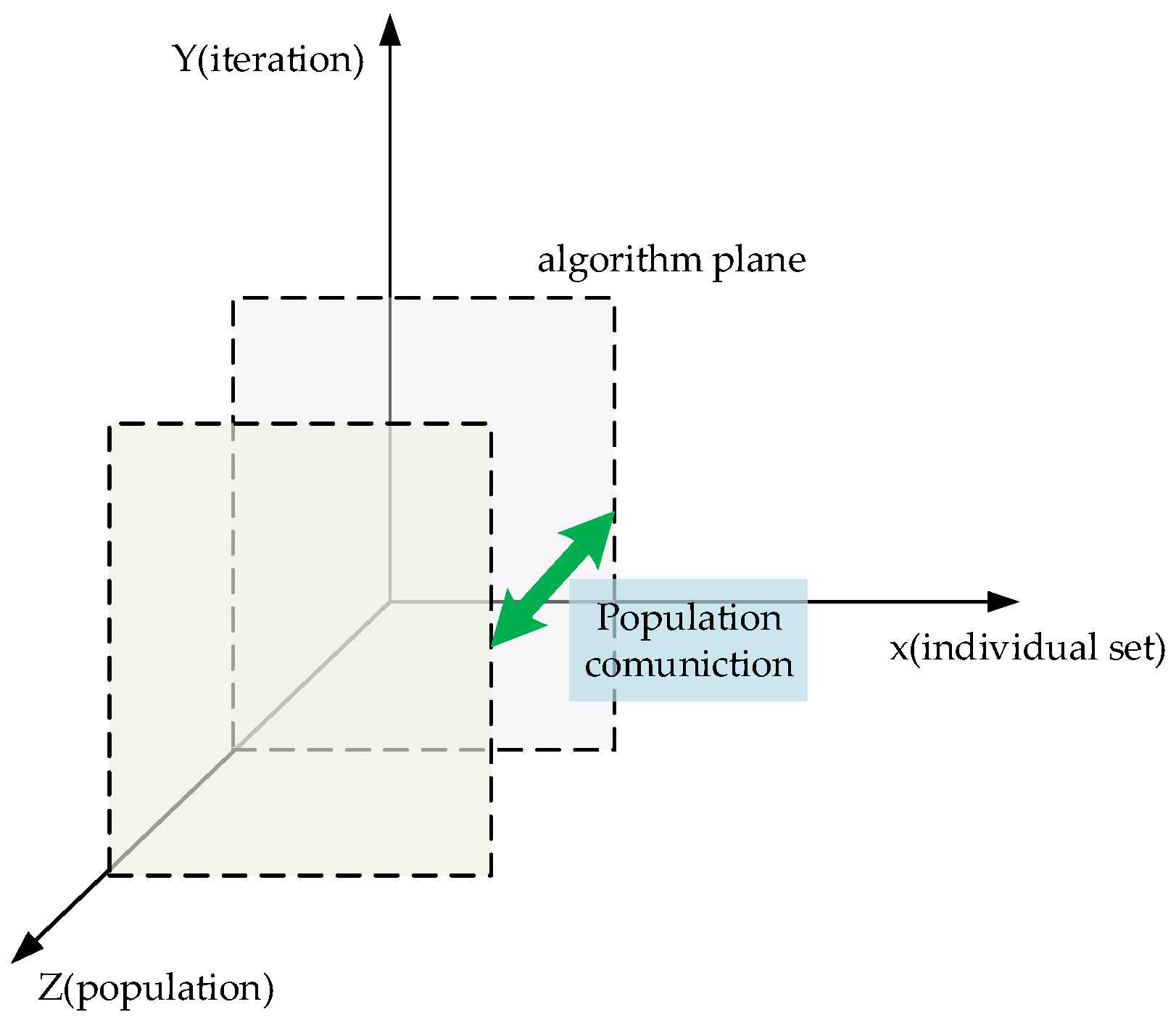
Any population-based intelligent optimization algorithm requires a population with multiple individuals. The algorithm needs to perform iteration in the search process. The individual of the population evolves according to the algorithm mechanism in each iteration. Some algorithms simulate complex multi-population model, and multiple populations coexist and communicate by specific communication mechanisms. Therefore, a population-based intelligent optimization algorithm can be considered as a three-dimensional model, as shown in Figure 1. We consider the population-based optimization algorithm to be a three dimensional structure: x-dimension, y-dimension, and z-dimension; where x represents the individual dimension of the population, y represents the iterative dimension of the loop, and z represents the parallel population dimension. The x-y forms an algorithm plane that can search independently. Multiple algorithm planes are parallel on the z-dimension and influence each other by exchange individuals. A simple algorithm degenerates to a point in the z-dimension, meaning a single population, and has the same behavior in both the x- and y-dimensions, representing that the algorithm has only one behavior. Current algorithm research tends to improve algorithm performance and robustness through a combination of multiple behaviors. From the three-dimensional model, it can be seen that each dimension can be combined with different behaviors, and a combination of behaviors in different dimensions contains a different optimization idea that should bring different effects. This article divides the multi-behavior combination into three levels:
- (1)
- Individual level: the combination of multiple behaviors at individual level refers to that individuals of a population may have different behaviors. Each individual selects a specific behavior according to certain rules. Individual level combination is a combination of ways to bring richer behaviors in a population and can make the entire population more diverse.
- (2)
- Iteration level: the combination of multiple behaviors at iteration level means that different evolutionary generations may use different behaviors during evolutionary process. The multiple behaviors can be related to different stages according to their evolutionary state, or be executed alternately.
- (3)
- Population level: the combination of multiple behaviors at the population level means that each sub-population may have its own behavior. In this combination, each sub-population is independent, and a sub-population communication mechanism is needed.
2.2. Behavior
Different algorithms or algorithm components are used to represent particular behaviors. The combination of multiple behaviors can be a combination of algorithms or algorithm components. Algorithm component is constituent element of the algorithm. For multi-behavior combination, it is necessary to extract the behavior pattern from the algorithms in unit of one iteration which we called the operator of an algorithm. Since the algorithm is a population-based algorithm, the core operator is individual (population) evolution operator, which represents an evolutionary behavior from the parent individuals (population) to the child individuals (population). Some algorithms can be further decomposed to extract the auxiliary operators, which are the certain technological elements of an algorithm such as parameter control strategy, constraint processing technology, etc., and can also be used as the combination elements. This paper categorizes the behaviors into the following six types of operator:
- (1)
- Individual (population) evolution operator: individual (population) evolution operator is the core operator of various algorithms. Most algorithms are based on individual evolution, and a small number of algorithms are the overall population evolution, such as CMA-ES [49]. The operator directly operates on the individuals or population to generate the offspring.
- (2)
- Parent individual selection operator: the parent individual is the individual which applies in individual evolution operation; therefore, it is an auxiliary operator for an individual evolution operator, such as random selection, selection based on individual topology, selection based on fitness, selection based on distance, etc.
- (3)
- Population selection operator: the operator selects the individuals entering the next generation between the parent population and the offspring population. A variety of population selection strategies have been adopted in the algorithms. The PSO algorithm directly uses the offspring population as the next generation population, the DE algorithm adopts the binary selection, the GA adopts the fitness-based selection, and some studies improve the population selection with considering the diversity.
- (4)
- Parameter control operator: the parameter control operator is used to set the parameter values of the algorithm. The parameter control operator also acts as a behavior because different parameter values can cause different search trajectory. The current research has proposed a variety of parameter control strategies. Some algorithms use fixed parameters, and some use only simple strategies, such as random values, descending linearly by evolution generation. Some studies proposed adaptive parameter control strategies. Some of these strategies are general and can be extracted as operators.
- (5)
- Population size control operator: population size is also a parameter of the algorithm, but it has great difference from the operation related parameters. It can also affect the population behavior. Thus, population size control strategy can also be extracted as an operator.
- (6)
- Constraint processing operator: the population-based intelligent optimization algorithm is suitable for solving single-object unconstrained (boundary constraint) optimization problems. Additional mechanisms are needed for constraint processing when solving constrained optimization problems. The most straightforward approach is to discard the infeasible solution, but this approach may lose performance, because infeasible solutions also carry valid information, and when the search space is not continuous, the intelligent optimization algorithm may fall into local extrema. Therefore, some studies explore constraint processing techniques. Generally, constraint processing occurs at the population selection step, therefore, it can be embedded into the population selection operator to construct the constraint-based population selection operator.
The multi-behavior combination can be an ensemble of multiple individual evolution operators, or multiple auxiliary operators, or an ensemble of multi-type multiple operators.
2.3. Combination Strategy
In addition to three combination modes, a combination of multiple behaviors also needs to establish corresponding combination strategies. For individual level combination, each individual’s behavior is needed to be determined; and for the combination at iteration level, each evolutionary generation is needed to determine the behavior for it; and the combination at population levels should determine sub-population behavior, and establish sub-population communicate mechanism. In this paper, we adopt the reverse thinking to take the behavior as the core. For an ensemble of behaviors, if individual level combination is used, individual groups should be determined for each behavior, including group size and grouping methods; if an iteration level combination is used, evolutionary generations should be determined for each behavior; and if population level combination is used, sub-population (is also an individual group) should be determined for each behavior including communication mechanism. Thus, each behavior has its individual group, evolutionary generations, and change strategy. Thereby, the behavior combination can be unified in a general framework. The combination of multiple behaviors can be in a competitive or collaborative manner.
2.3.1. Collaborative Strategy
The collaborative strategy means that the related behaviors have a cooperative relationship, that they will support each other. The collaborative relationship is generally pre-customized, and the goal of collaboration is achieved through different search characteristics of multiple behaviors. Therefore, according to the behavior characteristic, the individual group, or generations, or communicating mechanism can be defined under specific combination mode. The communication mechanism of individual groups can be re-grouping (which is more suitable for individual level combination), or migrating and mixing individuals between different individual groups (which is more suitable for population level combination).
2.3.2. Competitive Strategy
The competition strategy means that multiple behaviors compete with each other and decide the winner. The winner would acquire more resources as the reward. The competitive resource of the individual level combination is the number of individuals, and the resource of the iteration level combination is execution probabilities. The population level combination is generally suitable for the collaborative strategy, but the sub-populations can also compete for the amount of communication resources.
Although the resources to be competed are different, they can be unified. We define the resources for competition as probability, that is, the resource occupancy rate of each behavior. It is defined as a vector P = {P1, P2,... Pm}, m is the number of behaviors, and Pi is the resource occupancy of the ith behavior, 1 ≤ i ≤ m. The basis of the competition strategy is the evaluation model of behavior. Define evaluation model data for all behaviors as a vector soState = {soState1, soState2, …, soStatem}, soStatei is the model score for the ith behavior, and soStatebest is the score for the optimal behavior.
The paper gives two competing strategies, one is a full-competitive strategy and the other is a semi-competitive strategy. The full-competitive strategy maximizes the resources of the excellent behavior set, and the definition of the excellent behavior set is shown in Equation (1), Pi is adjusted according to Equations (2) and (3) [50], rate is the maximum adjustment ratio.
The semi-competitive strategy defines a base ratio vector Pbase = {Pbase,1, Pbase,2,.., Pbase,m}, and Pbase,i defines the resource ratio that the ith behavior at least occupies. The remaining ratios are proportionally assigned based on the model scores of the behaviors. The adjustment method of Pi is as follows:
2.4. Evaluation Model
Two kinds of evaluation may be needed in the process of behavior combination. One type of evaluation is to evaluate the population in order to understand the evolution state and select the appropriate algorithm. The other type of evaluation is the evaluation of behavior since the optimization performance of each behavior needs to be known for the competitive strategy. It may be necessary to decide which behavior is the winner based on the relative performance of multiple behaviors. Both types of evaluation are judged according to the population. Various evaluation mechanisms are established through the relevant information of the parent population and its offspring population. We divide the evaluation mechanism into two categories:
2.4.1. Fitness Based Evaluation
The evaluation mechanism based on fitness is a more intuitive evaluation mechanism. Obtaining the optimal fitness is the goal of the algorithm. Therefore, the fitness evaluation mechanism is suitable for evaluating the performance of the behavior.
(a) Success rate (SR). The SR refers to the successful improvement rate for offspring to parent population. It is as follows:
where NP is the individual number of the population, SI is the set of individuals which enter the next generation from offspring population, and |SI| means the individual number of SI.
(b) Successful individual fitness improvement mean (SFIM). The SFIM is a mean value for all successful individual. If the population selection operator is binary selection as DE used, it can be computed as Equation (7). If the population selection operator is not binary selection, the Equation (8) can be used.
where ∆fk is the fitness improvement value of the offspring individual uk,g to the parent individual xk,g. f is the fitness function (objective function), SI has the same meaning with Equation (5), and PI is the set of parent individuals being replaced.
2.4.2. Evaluation Based on Other Information
Although the evaluation mechanism based on fitness is the most direct and effective method, it lacks other state information of the reference population. Considering the population performing the optimization as a stochastic system, information entropy can be used to evaluate the state of the population. Information entropy can be seen as a measure of system ordering, and the changes in entropy can be used to observe changes in populations. We also adopt an evaluation model based on information entropy measurement in the target space. The information entropy for discrete information is shown as follows:
where n represents the number of discrete random variables, and pi represents the probability of the ith discrete random variable, pi ∈ [0,1], and p1 + p2 +...+ pn = 1.
Let NP to be the individual number of the population, and the maximum and minimum objective values of the population are fmin, fmax. Divide [fmin, fmax] in the target space into NP sub-domains as the NP discrete random variables. Then pi is the individual percentage of the ith sub-domain.
where ci represents the number of individuals with objective values in the ith sub-domain. H is the information entropy of the population representing the population diversity.
According to the multi-behavior combination model, a multi-behavior combination algorithm can be defined according to Table 1.
3. Agent-based General Algorithm Combination Framework
In order to customize the multi-behavior combination algorithm conveniently, the model needs to be designed as a framework. In this section we construct an agent-based general framework.
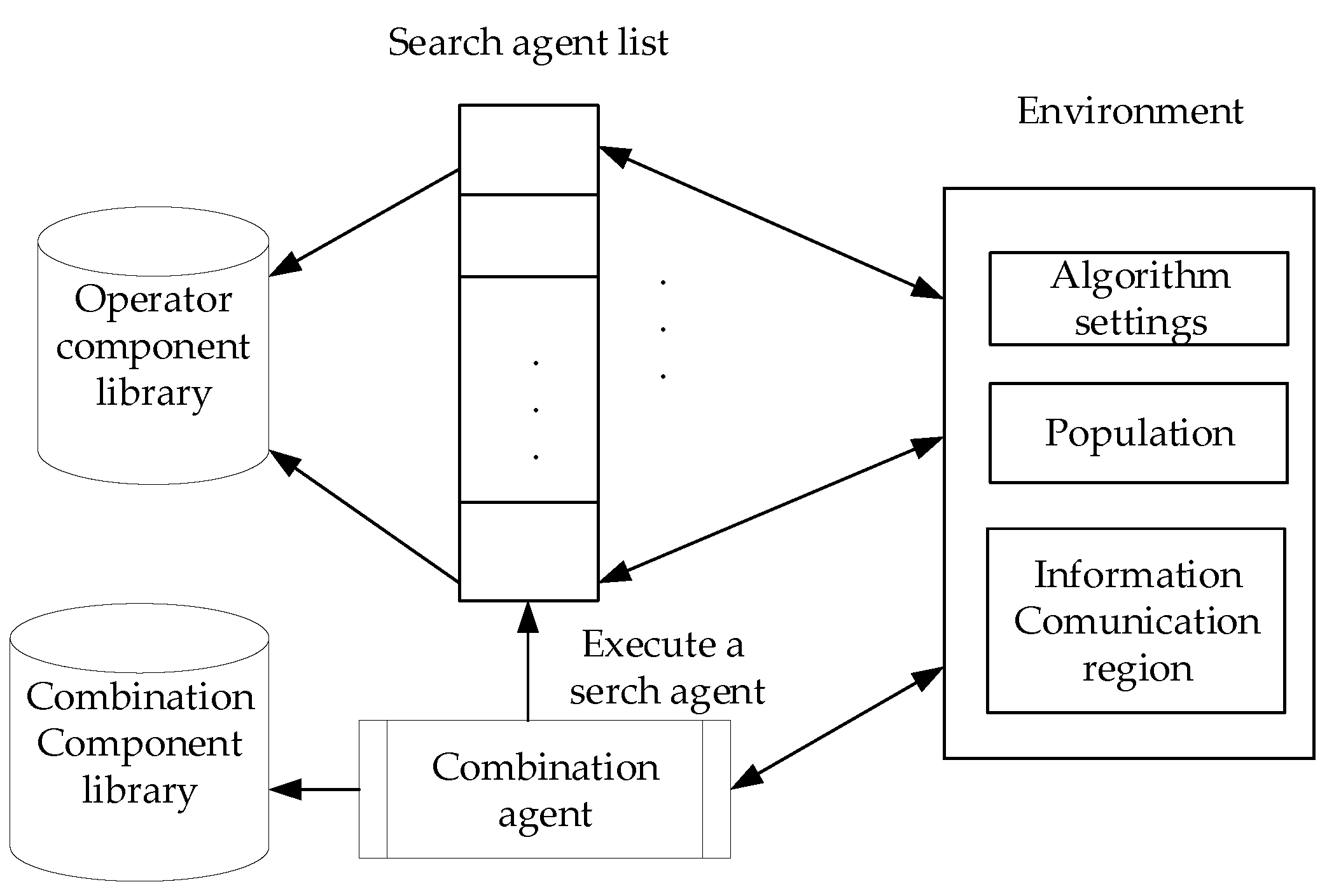
First, an operator component library is built for the operators that represent various candidate behaviors. The core of the framework is to construct the search agent which represents a behavior in runtime. Multiple behavior set are expressed by a search agent list. Therefore, operators that implement a behavior are encapsulated in a search agent. Each search agent is autonomous and can perform the search in a centralized or distributed environment independently. The combination of algorithms or combination of operator components is transformed into a combination of search agents. Multi-behavior combination is modeled by a combination agent which describes the combination scheme and determines the execution logic in order to schedule the search agents. The combination component library includes some related combination modes and strategies. A multi-agent system environment is defined for information exchange among search agents, including the entire population information, general settings of algorithm, information communication region. The framework structure is shown in Figure 2.
3.1. Operator Component Library
The operator components in the operator component library are designed or extracted from existing algorithms. The six types of operators summarized in Section 2.2 can be embedded in the framework. A uniform interface for each type of operator is defined. Each operator takes one iteration as the extraction unit. The data structure corresponding to an operator component should be constructed if some information needs to be maintained between the two iterations of the operator. Most algorithms have the same structure on evolution operation: at first parent individual selection, then individual evolution to generate offspring, finally population selection. These algorithms can be decomposed into the three types of operator components if they are general and can be reused. And these algorithms can be assembled by the corresponding operator components when in runtime. There are also algorithms that cannot be decomposed to general components, thus, the entire evolution operation in one iteration can be extracted into an independent individual evolution operator component.
3.2. Search Agent
Each search agent represents a behavior that can search independently, and therefore, it is an iterative unit of a complete algorithm. It contains the information needed by a complete algorithm, and is defined as a five-tuple:
SAinfo = (AlInfo, GroupInfo, RuntimeInfo, OffspringInfo, ModelInfo)
- AlInfo is a data structure for algorithm information. The algorithm information describes its corresponding operator combination. The individual evolution operator is the core operator. According to the core operator, the auxiliary operators (parent individual selection operator, the population selection operator) are selected if needed, then the parameters of the algorithm can be determined, and the parameter control operator can be selected.
- GroupInfo is a data structure for individual group information. It means the population of an algorithm, including the group size, individual set, individual type.
- RuntimeInfo is a data structure for runtime information. Runtime information comes from the algorithm running process, because some information should be retained during the iteration. Various operator components may require their specific information; thus, the related runtime information structure is constructed when the operator component is executed for the first time.
- OffspringInfo is the result of search behavior, and it represents the set of offspring individuals.
- ModelInfo is the evaluation data of the behavior. It is a vector including one or more selected evaluation models from {SR, SFIM, Entropy}.
A single-step search behavior is defined to enable the search agent to run step by step. The algorithm is identical for all search agents, and the difference is the operators and group. The algorithm is showed in Algorithm 1.
| Algorithm 1. Single-step behavior of search agent. |
| Input: AlInfo, GroupInfo, RuntimeInfoOutput: OffspringInfo, ModelInfo foreach parameter strategy in AlInfo Execute the parameter strategy operator component to generate the parameter value set. end foreach Execute the evolution operation (including an operator list in AlInfo) and return the offspring set. Compute the objective of the offspring. foreach parameter strategy in AlInfo Execute the parameter strategy component to collect information and construct the parameter strategy model. end foreach Collect the algorithm information to generate ModelInfo. |
3.3. Combination Agent
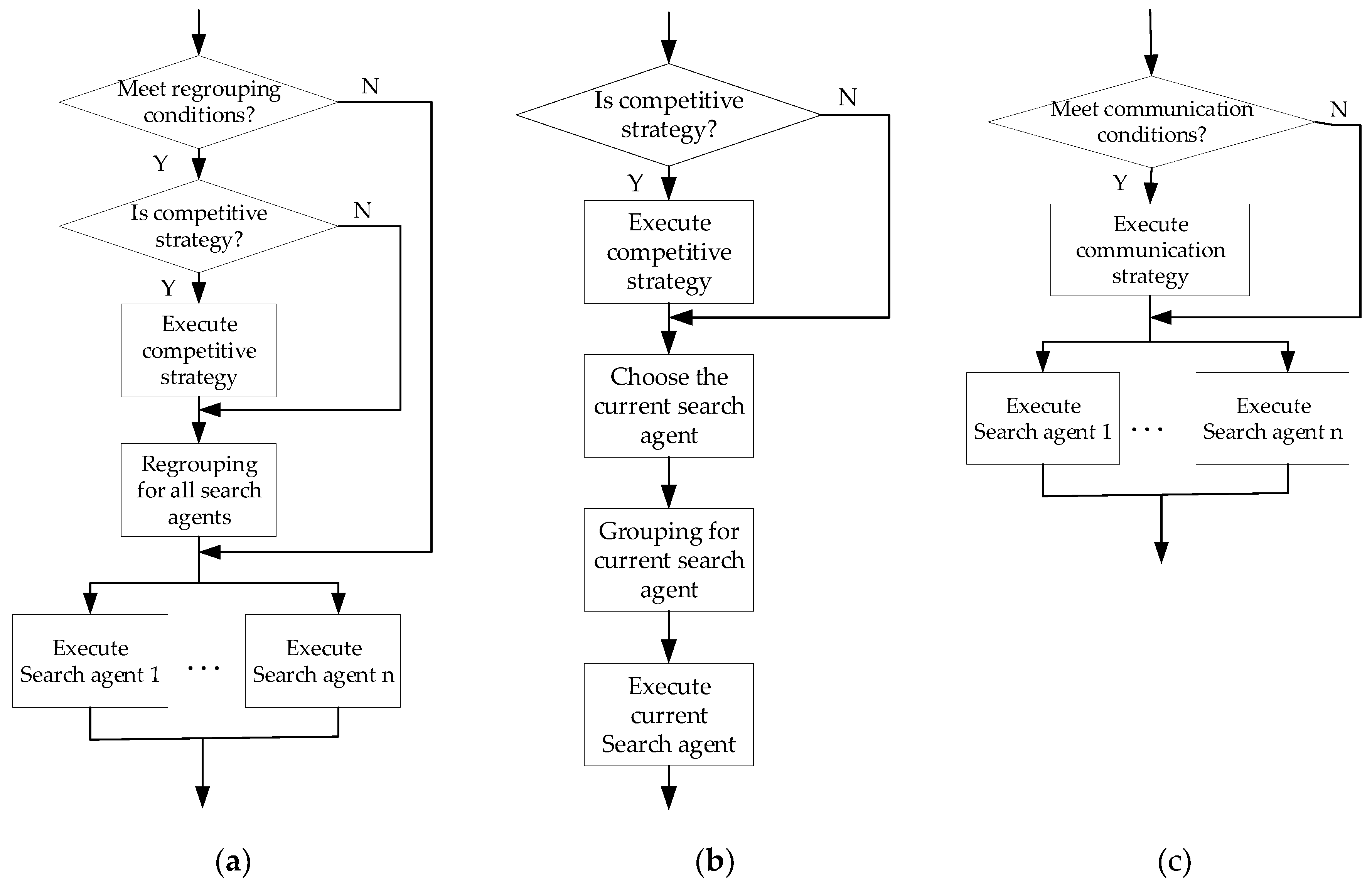
The combination agent includes the data structure for describing the combination scheme and the algorithm for executing the combination mechanism. Each search agent represents a specific behavior. The combination scheme defines the combination mode and combination strategy for multiple behaviors (multiple search agents). In the framework, we predefined three basic combination modes as {individual level combination, iteration level combination, population level combination}. Each combination mode needs to define its population grouping strategy and execution strategy, which determines the individual group and execution manner for all search agents in a combination mode. The predefined strategies are shown in the Table 2 and are supported by the combination component library which includes the three combination mode components, grouping components, competitive strategy components, group communication components. The flow chart of three combination mode components in one iteration is shown in Figure 3. It can be seen that the other strategy components are called by the combination mode components. The combination agent executes corresponding combination mode components according to the combination scheme described.
3.4. Algorithm Reuse and Algorithm Customization under the Framework
Most population-based optimization algorithms can be integrated into the framework. In this paper, an algorithm that adopts the same behavior in three dimensions is called a single-behavior algorithm. An algorithm that adopts different behaviors in any dimension is called a multi-behavior combination algorithm. Most existing algorithms can be classified as single-behavior algorithms or multi-behavior combination algorithms.
Both single-behavior and multi-behavior algorithms can be decomposed to extract the six types of technical unit operators if they have. For the multi-behavior combination algorithms, the combination modes adopted by the algorithms generally belong to the three basic combination modes. However, the combination strategy may be various. We predefined some combination strategies, which may also be extracted as components from the current multi-behavior algorithms and reused by the combination agent.
By analyzing the behaviors and the combination method of the existing algorithms, the operator components and the combination strategy components are extracted, and the existing algorithms can be recombined in the framework. More importantly, the new algorithm can be customized under the framework.
Customizing an algorithm first requires the determination of the optimization idea of multi-behavior combination, selection of the corresponding operators, and the combination of related operators into multiple search agents. Then, the combination scheme is designed, including combination mode, combination strategy, grouping strategy, and some fixed parameters. Then, the algorithm can be executed by the framework. The algorithm of the framework is as Algorithm 2.
| Algorithm 2. Algorithm of the framework. |
| Initialize the algorithm settings (population size, max evaluation number, boundary constraint). Construct the data structure of combination scheme. Construct the data structure of each search agent and generate search agent list. Initialize the population and evaluation by objective function. while (not satisfied the termination condition) execute combination agent acquire the combination mode according to combination scheme data structure. execute the corresponding combination mode component (Figure 3). end combination agent record the best result end while |
To demonstrate the working principle of this framework, we give the examples on introducing DE and its variants jDE [51], SHADE [52], and teaching-learning-based optimization algorithm (TLBO) [29] into the framework:
3.4.1. DE, jDE and SHADE
At first, the individual evolution operator, the parent individual selection operator, the population selection operator, and the parameter control operator can be extracted from the three algorithms as operator components. The DE and jDE has the same individual evolutionary operator: DE/rand/1 mutation strategy and the binomial crossover strategy. The individual evolution operator of the SHADE algorithm adopts the DE/current-to-pBest/1 mutation strategy and binomial cross strategy. The DE and jDE also have the same parent individual selection operator: random selection. The parent individual of SHADE has two types, one is the best parent individual, the other is the ordinary parent individual. The best parent individual selection operator adopts a random selection among the top p% individuals (sorted by fitness), and the ordinary parent individual selection operator adopts a random selection among population and failure individual archive. For the population selection operator, the three algorithms all use binary greedy selection. For the parameter control operator, DE uses the fixed value strategy, jDE and SHADE use adaptive parameter control strategies [51,52], which can be reused and are suitable to be extracted as operator components.
The three algorithms are all single-behavior algorithms. When using one of them, the related operator components can be selected and assembled into a search agent. For example, the SHADE algorithm has four operator components. The identifier (ID) of each component is specified in the AlInfo structure of the search agent. Algorithm 1 automatically calls the corresponding component for an iterative execution. The predefined execution order of operator components is: (1) execute the parameter components for the first call and generate the parameter value set, (2) execute the best parent individual selection component to generate the optimal parent individual set, (3) execute the ordinary parent individual selection component to generate other parent individual set, (4) execute the individual evolution component to generate the offspring, (5) execute the population selection component to generate the population of next generation, (6) execute the second call of the parameter control component to generate the parameter strategy model (needed by adaptive parameter control strategy), and (7) execute the algorithm evaluation component and generate algorithm evaluation model. If any step is not required, the component ID is set to 0, and the step is skipped. The search agent is called by the framework iteratively; thus, the SHADE algorithm can be supported by the framework.
3.4.2. Teaching-Learning-Based Optimization (TLBO)
TLBO algorithm is a multi-behavior combination algorithm. It contains two behaviors in the iteration level, one is teaching behavior and the other is learning behavior. It can be introduced into the framework by four steps: (1) extract operators for each behavior; (2) select the operator components and construct the search agent for each behavior with description in AlInfo of each search agent; and (3) define the combination method of the two behaviors and describe it in the data structure of the combination agent. For the TBLO algorithm, the combination mode is an iteration level combination. For this combination mode, it does not need to divide the population for the search agents. It only needs to assign individuals according to the GroupInfo of the search agent. The group of the two behaviors in the TLBO algorithm is the entire population which can be described by the GroupInfo. The multi-behavior combination strategy is a collaborative strategy, the search agents are executed in a predefined fixed order: one by one. (4) The framework executes the combination agent iteratively, and the combination agent calls the component for iteration level combination. The algorithm flow of the component for iteration level combination is showed in Figure 3b.
Most of the algorithms adopt one combination mode for multiple behavior and can be customized by simple settings under the framework. However, a few studies explore the more complex combination, which can be seen as a further combination of these three basic combination modes. The components of the framework can also be reused to construct complex multi-level combination algorithm; however, the combination agent may need some modification.
4. Economic Load Dispatch Model and Algorithm Customizing
4.1. The Model of Economic Load Dispatch Problem
Economic load dispatch is a typical optimization problem in power systems. The goal is to minimize fuel costs by rationally arranging the active power output of each generating unit in a power plant or power system on the premise of meeting system load demand and operational constraints.
4.1.1. Problem Definition
The objective function of the optimization problem is as follows:
where F is total fuel cost, Ng is the total number of online generating units of the system, Pi is the power output (in MW) of ith generator, Fi(Pi) is the cost function of the ith generator as Equation (12), if the valve point effect is considerd, Fi(Pi) can be described as Equation (13).
where ai, bi, ci, ei, fi is the cost coefficients of the ith generator.
In addition to the objective function, the problem needs to meet some constraints:
4.1.2. Generator Output Constraint
4.1.3. Power Balance Constraints
4.1.4. Ramp Rate Limit Constraints
4.1.5. Prohibited Operating Zones Constraints
The generating units may have certain zones where operation is restricted. Consequently, the feasible operating zones are discontinuities as follows:
where ni is the total number of prohibited operating zones, Pi,jpzl and Pi,jpzu are the lower and upper limits of the jth prohibited zone for the ith generating unit respectively.
4.2. Customizing Multi-Behavior Combination Algorithm
The algorithm we customized for ELD problem is a multi-behavior combination algorithm. The behaviors come from the operator component library. At present, we only give small number of operators including some individual evolution operators (mainly DE algorithm operator and its invariants including mutation step and crossover step), some parent individual selection operators, some parameter control operators, and a population selection operator (just DE adopted) and its two constraint-based version with penalty functions method [45] and ε-constraint handling method [45].
The ε-constraint handling method gives the constraints a relaxation scope, and if the constraint violation value of individuals are less than ε, the individuals are considered feasible. Then in the population selection operator (an operator of one-to-one choice between parent individual and offspring individual), two feasible individuals are compared and selected according to objective value, and in the other case, individuals are selected according to constraint violation degree. The ε is varied as follows [45]:
where ε(0) is the initial ε value, Xθ is the top θth individual and θ = (0.05 × NP), v is constraint violation function. cp and Tc are parameters, and Tc is a specific generation in iteration.
For the multi-behavior algorithm, we give three behaviors which come from DE algorithm and its variants jDE [51], SHADE [52], etc. The three behaviors are constructed with the operators in the operator component library. The design for behaviors is showed in Table 3. Behavior1 and behavior2 have the similar algorithms with difference in parameter control operator. Behavior2 and behavior3 have the similar parameter control operator with difference in algorithm operation. Behavior 1 is used for randomness and diversity. Behavior2 is a fitness improvement instructed search because its parameter control strategy tends to the parameter values which bring larger fitness improvement. Behavior 3 is an optimal individual set instructed search, and is used for gathering in the optimal regions. The combination method of the three behaviors is designed as Table 4. Based on the combination method in Table 4, the three behaviors are executed in a fixed order from behavior 1 to 3 for the iteration level, so the search process is a repeated local small loop from diversity exploration to exploitation.
Just like the example in Section 3.4, the three behaviors are organized as search agents. It only needs to describe the operator components designed in Table 3 with AlInfo of search agent, then the search agent can execute these components in order with one iteration. However, the execution manner of multiple search agents is determined by the design in Table 4. The combination agent interprets the combination design and executes the search agents in a designed manner. The combination method is similar to the TLBO algorithm, but we have three behaviors. The behavior combination happens at the iteration level and the combination strategy is collaborative strategy which adopts the fixed execution manner: the three behaviors are executed one by one.
The algorithm of this paper is a general constrained optimization algorithm. The optimization objective is Equation (11). Xi = {Pi,1, Pi,2,…Pi,Ng} is an individual vector, and is also a solution of the ELD problem, which means the power outputs of all the online generating units. In the current population-based intelligent optimization algorithm for solving ELD problems, the constraint processing can be divided into two categories. One is to process the individuals that violate the constraints and use the problem-specific knowledge to modify the individuals and satisfy the constraints as much as possible. However, because the constraints are more difficult to fully satisfy, the algorithm still needs to provide constraint processing technology. Another type of algorithm does not perform special processing, but only uses general constraint processing techniques. In this paper, the constraint of Equation (14) is processed as boundary. When the transmission loss is not considered, the equality constraint is simply processed according to Equation (15) by recomputing the power output of the last generating unit, and the other inequality constraints are not processed. When considering the transmission loss, the constraint relationship is complicated, and we do not make special treatment, the constraints are processed only through the ε-constraint handling method. The tolerance of the equality constraint is set as 10–4, which can be updated according to the problem. In order to facilitate the comparison, the algorithm proposed by this paper is named as multi-behavior combination differential evolution algorithm (MBC-DE).
5. Experiment and Discussion
In this section, the proposed algorithm and framework is applied in ELD problems. The ELD problem is a non-convex, nonlinear, discontinuous constrained optimization problem. The equality constraint involved is power balance constraint, inequality constraints are ramp rate limit constraints, and prohibited operating zones constraints. The valve point effect may or may not be considered in the objective function, and transmission losses may or may not be considered in the equality constraint. The transmission losses are calculated by B-coefficient method. We use four test system which varies with different difficulty levels. For each test case, 20 independent runs are performed and the results of the best, worst and mean fuel costs are recorded and compared with other algorithms. Each behavior of the multi-behavior algorithm is tested independently in order to analyze the effects of the multi-behavior combination. The three single-behavior algorithms are named as Behavior1~Behavior3. The population size is set as 50 for all cases, and the max iteration is 2000 generation.
(1) Test Case 1: Test case 1 is a small system. The system is comprising six generators, and the ramp rate limit, prohibited operating zone and transmission losses are all considered without valve point loading effect. The system data is from [2,3]. The load demand is 1263 MW.
Table 5 gives the best output for this case, it can be seen that the equality constraint accuracy is less than 10-4, and all the inequality constraints are satisfied (see the system data in [2]). Table 6 give the comparison between single behavior and multi-behavior algorithm. Among the three behaviors, Behavior3 performs best, and MBC-DE inherits its characteristics and obtains a smaller standard deviation. Table 7 give the comparison between MBC-DE and other algorithms. From the data in the table, the algorithm MBC-DE goes beyond some algorithms, but there are also some algorithms that are better than MBC-DE. In test case 1, MBC-DE falls into a local extremum. The three sub-algorithms of MBC-DE are all differential evolution and the search trajectory is similar. No behavior can help MBC-DE to jump out of this local extremum. This also give us the confidence on algorithm combination research by introducing new algorithm or algorithm components into the framework, to enrich the algorithm behaviors.
(2) Test Case 2: Test case 2 is a 15 units system. The ramp rate limit and transmission losses are considered. There are 4 generators having prohibited operating zone. The valve point loading effect is neglected. The system data is also from [2,3]. The load demand of the system is 2630MW.
Table 8 gives the best output of MBC-DE for this case, it can be seen that the equality constraint accuracy is also less than 10-4, and all the inequality constraints are satisfied (see the system data in [2]). Table 9 give the comparison between single behavior and multi-behavior algorithm. Among the three behaviors, Behavior3 still performs best, and MBC-DE is better than Behavior3 in mean and worst value. We believe this is due to the combination of multiple behavior, although Behavior2 and 1 is worse than Behavior3. Table 10 shows the comparison between MBC-DE and other algorithms. The data in the table shows that the algorithm we proposed achieved better results than others in case 2.
(3) Test Case 3: test case 3 is a 40 units system with valve point effect being considered. The ramp rate limit and transmission losses are neglected. The load demand is 10,500 MW. The system data is from [4].
Table 11 gives the best output of MBC-DE for this case; it can be seen that the equality constraint is satisfied. Table 12 give the comparison between single behavior and multi-behavior algorithm. Among the three behaviors, Behavior1 and Behavior2 all performs well, and MBC-DE is better than them. We think the Behavior3 act as the supporting role, although it works poorly on its own. Table 13 give the comparison between MBC-DE and other algorithms. The data in the table show that the algorithm we proposed achieved better results. For the best value, MBC-DE is better than others, but for the mean value, MDE and DE/BBO are better.
(4) Test Case 4: test case 4 is a large-scale power system with 140 generators. The valve point effect is considered. The ramp rate limit and transmission losses are neglected. The load demand is 49,342 MW. The system data is from [59].
Table 14 gives the best output of MBC-DE for this case; and the equality constraint is satisfied. Table 15 give the comparison between single behavior and multi-behavior algorithm. Among the three behaviors, Behavior3 has the best result and the worst result, this means that the algorithm has large fluctuations and instability. MBC-DE has improved in both the optimal value and stability which represents the effect of algorithm combination. Table 16 gives the comparison between MBC-DE and other algorithms. The data in the table show that the algorithm we proposed achieved better results.
Implementing the algorithm in the form of a framework maybe lose some efficiency. The reason is that in order to achieve generality and easy assemblage, various technical units need to be designed as components which can be implemented as functions in Matlab, and thus the overhead of function call is generated. This gap can be reduced through programming technology. In fact, the running time of the algorithm is less than 30s with Matlab R2018a environment on a 1.99 GHz, 16 GB RAM Notebook computer. The time is feasible for some online systems. If the system has strict real-time requirements, the framework can also be used as a debugging tool to determine the algorithm. Then, code refactoring can be performed. The algorithm we proposed is not restricted by the constraint form and has a certain versatility.
6. Conclusions
Through the experiments in this paper, we can see that the performance of the population-based intelligent optimization algorithm can be improved by appropriate multi-behavior combination. A behavior has specific search trajectory, so it is easy to trap into the same local extremum. Multiple behaviors have different search trajectories, and can lead to more diversity, so the combination of multiple behaviors is more likely to be suitable for complex optimization problems. The ELD Problem has a complex solution space caused by multiple constraints, the algorithms are prone to trap into the local extremum. From the related research, it can be seen that different algorithms are gradually improving the optimization results, which also shows that the previous algorithm has fallen into the local extremum. Therefore, combining the search characteristics of different algorithms makes it possible to obtain good results. The algorithm in this paper is a combination of three DE variants. From the test results, the proposed algorithm with multiple behaviors is better than the single behavior used by the algorithm. However, the sub-algorithms all belong to the DE algorithm, thus, their search trajectories are similar, the algorithm results are improved only a little, and some studies have yielded better values. This makes us more convinced of the significance of implementing a multi-behavior combination framework. With more candidate behaviors, the algorithm may be improved further. Therefore, our follow-up work is to introduce more algorithms into the framework to enrich the candidate behaviors. Another research opportunity involves improving the multi-behavior combination strategy.
Multi-behavior combination is an important research idea of current intelligent optimization algorithms. This article hopes to introduce this idea into practical applications. Different from the traditional research, the focus of this paper is to realize the idea as a general framework. Various algorithm components can be extracted from the all kinds algorithm and introduced into the framework. By performing behavior design and the combination method design, the new algorithm can be assembled. It brings convenience to the customization of new algorithms and to algorithm combination research more generally. Although the algorithm is tailored to solve the ELD problem, it is obvious that the framework can apply to other practical problems with simple customization.
Author Contributions
J.Z. did the programming and writing; Z.D. instructed the idea and writting.
Funding
This research received no external funding.
Conflicts of Interest
The authors declare no conflict of interest.
References
- Chiang, C.-L. Genetic-based algorithm for power economic load dispatch. IET Gener. Transm. Distrib. 2007, 1, 261–269. [Google Scholar] [CrossRef]
- Gaing, Z.-L. Particle swarm optimization to solving the economic dispatch considering the generator constraints. IEEE Trans. Power Syst. 2003, 18, 1187–1195. [Google Scholar] [CrossRef]
- Gaing, Z.-L. Closure to Discussion of ‘Particle swarm optimization to solving the economic dispatch considering the generator constraints. IEEE Trans. Power Syst. 2004, 19, 2122–2123. [Google Scholar] [CrossRef]
- Sinha, N.; Chakrabarti, R.; Chattopadhyay, P.K. Chattopadhyay. Evolutionary Programming Techniques for Economic Load Dispatch. IEEE Trans. Evol. Comput. 2003, 7, 83–94. [Google Scholar] [CrossRef]
- Chiang, C.L. Improved genetic algorithm for power economic dispatch of units with valve-point effects and multiple fuels. IEEE Trans. Power Syst. 2005, 20, 1690–1699. [Google Scholar] [CrossRef]
- He, D.K.; Wang, F.L.; Mao, Z.Z. Hybrid genetic algorithm for economic dispatch with valve-point effect. Electr. Power Syst. Res. 2008, 78, 626–633. [Google Scholar] [CrossRef]
- Mahdi, F.P.; Vasant, P. Quantum particle swarm optimization for economic dispatch problem using cubic function considering power loss constraint. IEEE Trans. Power Syst. 2002, 17, 108–112. [Google Scholar]
- Selvakumar, A.I.; Thanushkodi, K. A new particle swarm optimization solution to nonconvex economic dispatch problems. IEEE Trans. Power Syst. 2007, 22, 42–51. [Google Scholar] [CrossRef]
- Khamsawang, S.; Jiriwibhakorn, S. DSPSO–TSA for economic dispatch problem with nonsmooth and noncontinuous cost functions. Energy Convers. Manag. 2010, 51, 365–375. [Google Scholar] [CrossRef]
- Pothiya, S.; Ngamroo, I.; Kongprawechnon, W. Ant colony optimization for economic dispatch problem with non-smooth cost functions. Int. J. Electr. Power Energy Syst. 2010, 32, 478–487. [Google Scholar] [CrossRef]
- Noman, N.; Iba, H. Differential evolution for economic load dispatch problems. Electr. Power Syst. Res. 2008, 78, 1322–1331. [Google Scholar] [CrossRef]
- Panigrahi, B.K.; Yadav, S.R.; Agrawal, S.; Tiwari, M.K. A clonal algorithm to solve economic load dispatch. Electr. Power Syst. Res. 2007, 77, 1381–1389. [Google Scholar] [CrossRef]
- Secui, D.C. A new modified artificial bee colony algorithm for the economic dispatch problem. Energy Convers. Manag. 2015, 89, 43–62. [Google Scholar] [CrossRef]
- Dos Santos Coelho, L.; Mariani, V.C. An improved harmony search algorithm for power economic load dispatch. Energy Convers. Manag. 2009, 50, 2522–2526. [Google Scholar] [CrossRef]
- Al-Betar, M.A.; Awadallah, M.A.; Khader, A.T.; Bolaji, A.L. Tournament-based harmony search algorithm for non-convex economic load dispatch problem. Appl. Soft Comput. 2016, 47, 449–459. [Google Scholar] [CrossRef]
- Bhattacharya, A.; Chattopadhyay, P.K. Biogeography-based optimization for different economic load dispatch problems. IEEE Trans. Power Syst. 2010, 25, 1064–1077. [Google Scholar] [CrossRef]
- He, X.Z.; Rao, Y.Q.; Huang, J.D. A novel algorithm for economic load dispatch of power systems. Neurocomputing 2016, 171, 1454–1461. [Google Scholar] [CrossRef]
- Pradhan, M.; Roy, P.K.; Pal, T. Grey wolf optimization applied to economic load dispatch problems. Int. J. Electr. Power Energy Syst. 2016, 83, 325–334. [Google Scholar] [CrossRef]
- Lu, H.; Sriyanyong, P.; Song, Y.H.; Dillon, T. Experimental study of a new hybrid PSO with mutation for economic dispatch with non smooth cost function. Int. J. Electr. Power Energy Syst. 2010, 32, 921–935. [Google Scholar] [CrossRef]
- Niknam, T.; Azizipanah-Abarghooee, R.; Aghaei, J. A new modified teaching learning algorithm for reserve constrained dynamic economic dispatch. IEEE Trans. Power Syst. 2013, 28, 749–763. [Google Scholar] [CrossRef]
- Niknam, T.; Mojarrad, H.D.; Meymand, H.Z. A novel hybrid particle swarm optimization for economic dispatch with valve-point loading effects. Energy Convers. Manag. 2011, 52, 1800–1809. [Google Scholar] [CrossRef]
- Wang, L.; Li, L.P. An effective differential harmony search algorithm for the solving non-convex economic load dispatch problems. Int. J. Electr. Power Energy Syst. 2013, 44, 832–843. [Google Scholar] [CrossRef]
- Bhattacharya, A.; Chattopadhyay, P.K. Hybrid differential evolution with biogeography-based optimization for solution of economic load dispatch. IEEE Trans. Power Syst. 2010, 25, 1955–1964. [Google Scholar] [CrossRef]
- Mirjalili, S.; Lewis, A. The Whale Optimization Algorithm. Adv. Eng. Softw. 2016, 95, 51–67. [Google Scholar] [CrossRef]
- Meng, X.B.; Gao, X.Z.; Lu, L.H.; Liu, Y. A new bio-inspired optimisation algorithm: Bird Swarm Algorithm. J. Exp. Theor. Artif. Intell. 2016, 28, 673–687. [Google Scholar] [CrossRef]
- Meng, X.; Liu, Y.; Gao, X.Z.; Zhang, H.Z. A New Bio-inspired Algorithm: Chicken Swarm Optimization. In International Conference in Swarm Intelligence (ICSI 2014); Springer: Cham, Switzerland, 2014; pp. 86–94. [Google Scholar]
- Chu, S.C.; Tsai, P.W.; Pan, J.S. Cat Swarm Optimization. In Proceedings of the 9th Pacific Rim International Conference on Artificial Intelligence (PRICAI 2006): Trends in Artificial Intelligence, Guilin, China, 7–11 August 2006. [Google Scholar]
- Mirjalili, S.; Mirjalili, S.M.; Hatamlou, A. Multi-Verse Optimizer: A nature-inspired algorithm for global optimization. Neural Comput. Appl. 2015, 27, 495–513. [Google Scholar] [CrossRef]
- Rao, R.V.; Savsani, V.J.; Vakharia, D.P. Teaching-learning-based optimization: A novel method for constrained mechanical design optimization problems. Comput. Aided Des. 2011, 43, 303–315. [Google Scholar] [CrossRef]
- Yang, X. Flower pollination algorithm for global optimization. In International Conference on Unconventional Computation and Natural Computation (UCNC2012); Springer: Berlin/Heidelberg, Germany, 2012; pp. 240–249. [Google Scholar]
- Guohua, W.; Rammohan, M.; Nagaratnam, S.P. Ensemble strategies for population-based optimization algorithms—A survey. Swarm Evol. Comput. 2018, 9, 1–17. [Google Scholar]
- Wang, Y.; Cai, Z.X.; Zhang, Q.F. Differential Evolution with Composite Trial Vector Generation Strategies and Control Parameters. IEEE Trans. Evol. Comput. 2011, 15, 55–66. [Google Scholar] [CrossRef]
- Qin, A.K.; Huang, V.L.; Suganthan, P.N. Differential Evolution Algorithm with Strategy Adaptation for Global Numerical Optimization. IEEE Trans. Evol. Comput. 2009, 13, 398–417. [Google Scholar] [CrossRef]
- Li, X.T.; Ma, S.J.; Hu, J.H. Multi-search differential evolution algorithm. Appl. Intell. 2017, 47, 231–256. [Google Scholar] [CrossRef]
- Wang, S.C. Differential evolution optimization with time-frame strategy adaptation. Soft Comput. 2017, 21, 2991–3012. [Google Scholar] [CrossRef]
- Yi, W.C.; Gao, L.; Li, X.Y.; Zhou, Y.Z. A new differential evolution algorithm with a hybrid mutation operator and self-adapting control parameters for global optimization problems. Appl. Intell. 2015, 42, 642–660. [Google Scholar] [CrossRef]
- Elsayed, S.M.; Sarker, R.A.; Essam, D.L. Training and testing a self-adaptive multi-operator evolutionary algorithm for constrained optimization. Appl. Soft Comput. 2015, 26, 515–522. [Google Scholar] [CrossRef]
- Fan, Q.Q.; Zhang, Y.L. Self-adaptive differential evolution algorithm with crossover strategies adaptation and its application in parameter estimation. Chemom. Intell. Lab. Syst. 2016, 151, 164–171. [Google Scholar] [CrossRef]
- Wang, C.; Liu, Y.C.; Chen, Y.; Wei, Y. Self-adapting hybrid strategy particle swarm optimization algorithm. Soft Comput. 2016, 20, 4933–4963. [Google Scholar] [CrossRef]
- Gou, J.; Guo, W.P.; Wang, C.; Luo, W. A multi-strategy improved particle swarm optimization algorithm and its application to identifying uncorrelated multi-source load in the frequency domain. Neural Comput. Appl. 2017, 28, 1635–1656. [Google Scholar] [CrossRef]
- Wang, H.; Wang, W.; Sun, H. Multi-strategy ensemble artificial bee colony algorithm for large-scale production scheduling problem. Int. J. Innov. Comput. Appl. 2015, 6, 128–136. [Google Scholar] [CrossRef]
- Xiong, G.J.; Shi, D.Y.; Duan, X.Z. Multi-strategy ensemble biogeography-based optimization for economic dispatch problems. Appl. Energy 2013, 111, 801–811. [Google Scholar] [CrossRef]
- Cai, Y.Q.; Sun, G.; Wang, T.; Tian, H.; Chen, Y.H.; Wang, J.H. Neighborhood-adaptive differential evolution for global numerical optimization. Appl. Soft Comput. 2017, 59, 659–706. [Google Scholar] [CrossRef]
- Zhang, A.Z.; Sun, G.Y.; Ren, J.C.; Li, X.D.; Wang, Z.J.; Jia, X.P. A dynamic neighborhood learning-based gravitational search algorithm. IEEE Trans. Cybern. 2018, 48, 436–447. [Google Scholar] [CrossRef] [PubMed]
- Wang, Y.; Cai, Z.X. A Dynamic Hybrid Framework for Constrained Evolutionary Optimization. IEEE Trans. Cybern. 2012, 42, 203–217. [Google Scholar] [CrossRef] [PubMed]
- Wu, G.H.; Shen, X.; Li, H.F.; Chen, H.K.; Lin, A.P.; Suganthan, P.N. Ensemble of differential evolution variants. Inf. Sci. 2018, 423, 172–186. [Google Scholar] [CrossRef]
- Zhou, J.J.; Yao, X.F. Multi-population parallel self-adaptive differential artificial bee colony algorithm with application in large-scale service composition for cloud manufacturing. Appl. Soft Comput. 2017, 56, 379–397. [Google Scholar] [CrossRef]
- Wolpert, D.H.; Macready, W.G. No free lunch theorems for optimization. IEEE Trans. Evol. Comput. 1997, 1, 67–82. [Google Scholar] [CrossRef] [Green Version]
- Hansen, N.; Ostermeier, A. Completely Derandomized Self-Adaptation in Evolution Strategies. Evol. Comput. 2001, 9, 159–195. [Google Scholar] [CrossRef] [PubMed]
- LaTorre, A. A Framework for Hybrid Dynamic Evolutionary Algorithms: Multiple Offspring Sampling (MOS). Ph.D. Thesis, Universidad Polite’cnica de Madrid, Madrid, Spain, 2009. [Google Scholar]
- Brest, J.; Greiner, S.; Boskovic, B.; Mernik, M.; Zumer, V. Self-adapting control parameters in differential evolution: A comparative study on numerical benchmark problems. IEEE Trans. Evol. Comput. 2006, 10, 646–657. [Google Scholar] [CrossRef]
- Tanabe, R.; Fukunaga, A. Success-history based parameter adaptation for differential evolution. In Proceedings of the IEEE Congress on Evolutionary Computation 2013, Cancún, México, 20–23 June 2013. [Google Scholar]
- Chaturvedi, K.T.; Pandit, M.; Srivastava, L. Self organizing hierarchical particle swarm optimization for nonconvex economic dispatch. IEEE Trans. Power Syst. 2008, 23, 1079–1087. [Google Scholar] [CrossRef]
- Hosseinnezhad, V.; Babaei, E. Economic load dispatch using θ-PSO. Int. J. Electr. Power Energy Syst. 2013, 49, 160–169. [Google Scholar] [CrossRef]
- Yu, J.T.; Kim, C.H.; Wadood, A.; Khurshiad, T.; Rhee, S.B. A Novel Multi-Population Based Chaotic JAYA Algorithm with Application in Solving Economic Load Dispatch Problems. Energies 2018, 11, 1946. [Google Scholar] [CrossRef]
- Safari, A.; Shayegui, H. Iteration particle swarm optimization procedure for economic load dispatch with generator constraints. Expert Syst. Appl. 2011, 38, 6043–6048. [Google Scholar] [CrossRef]
- Hosseinnezhad, V.; Rafiee, M.; Ahmadian, M.; Ameli, M.T. Species-based quantum particle swarm optimization for economic load dispatch. Int. J. Elect. Power Energy Syst. 2014, 63, 311–322. [Google Scholar] [CrossRef]
- Amjady, N.; Sharifzadeh, H. Solution of non-convex economic dispatch problem considering valve loading effect by a new modified Differential Evolution algorithm. Int. J. Elect. Power Energy Syst. 2010, 32, 893–903. [Google Scholar] [CrossRef]
- Park, J.B.; Jeong, Y.W.; Shin, J.R.; Lee, K.Y. An improved particle swarm optimization for nonconvex economic dispatch problems. IEEE Trans. Power Syst. 2010, 25, 156–166. [Google Scholar] [CrossRef]
- Reddya, A.S.; Vaisakh, K. Shuffled differential evolution for large scale economic dispatch. Electr. Power Syst. Res. 2013, 96, 237–245. [Google Scholar] [CrossRef]
Figure 1.
A three-dimensional model for population-based intelligent optimization algorithm.

Figure 2.
Agent-based framework structure.

Figure 3.
The flow charts of three combination mode components in one iteration: (a) Individual level combination; (b) Iteration level combination; (c) Population level combination.
Figure 3.
The flow charts of three combination mode components in one iteration: (a) Individual level combination; (b) Iteration level combination; (c) Population level combination.


Table 1.
Multi-behavior combination algorithm attributes.
| Algorithm Attributes | Attributes Value Range |
|---|---|
| combination method | {individual level, iteration level, population level} |
| combination strategy | {collaborative strategy, competition strategy} |
| behavior operator set | {six categories of operators} |
| evaluation model | {SR, SFIM, Entropy, Compound model, none} |
Table 2.
Combination Scheme Settings.
| Combination Mode | Individual Group | Iteration (Execution Manner) | ||
|---|---|---|---|---|
| Group Size | Grouping Method | Group Communication | ||
| individual level | fixed full-competition semi-competition | Split the population | Regrouping (Every few generations) | every generation |
| iteration level | fixed | share the population | none | fixed full-competition semi-competition |
| population level | fixed | Split the population | migration of individuals (Every few generations) | every generation |
Table 3.
The multi-behavior design with operators.
| Behavior | Operator Components | Design |
|---|---|---|
| 1 | Individual evolution operator: | DE/rand/1 mutation strategy, Binomial crossover strategy (comes from DE algorithm). |
| Parent individual selection operator: | Random selection strategy. | |
| Population selection operator: | Binary selection (come from DE algorithm) with ε-constraints handling method (cp = 5, Tc = 0.7). | |
| parameter control operator: | F and CR: jDE algorithm strategy with parameter domain in [0,1]. | |
| other operators: | none | |
| 2 | Individual evolution operator: | The same as behavior 1 |
| Parent individual selection operator: | The same as behavior 1 | |
| Population selection operator: | The same as behavior 1 | |
| parameter control operator: | F and CR: SHADE algorithm strategy with parameter domain in [0,1]. | |
| other operators: | none | |
| 3 | Individual evolution operator: | DE/current-to-pBest/1 mutation strategy with archive, Binomial crossover strategy (come from SHADE algorithm) |
| Parent individual selection operator: | Best individual: random selection from %p top individual set with fitness sorting Other individuals: random selection from population and archive | |
| Population selection operator: | The same as behavior 1. | |
| parameter control operator: | p: linear decreasing strategy based on generation from 0.5 to 0F and CR: SHADE parameter control strategy with domain in [0,1] | |
| other operators: | none |
Table 4.
Behavior Combination design.
| Combination Settings | Design |
|---|---|
| combination mode | Iteration level combination. |
| group size | Fixed (NP: population size). |
| grouping method | Share (The entire population). |
| group communication | None. |
| iteration | Collaborative strategy: fixed (executed one by one) |
Table 5.
Best outputs for test case 1 with PD = 1263 MW (6-units system).
| Unit | 1 | 2 | 3 | 4 | 5 | 6 |
|---|---|---|---|---|---|---|
| Output power (MW) | 446.716 | 173.145 | 262.797 | 143.490 | 163.918 | 85.3562 |
| Total Power output (MW) | 1275.42190006 | |||||
| Transmission loss (MW) | 12.422 | |||||
| Fuel cost($/h) | 15,444.185 | |||||
Table 6.
Algorithm comparison between multi-behavior and single-behavior for test case 1.
| Algorithm | Cost ($/h) | std | ||
|---|---|---|---|---|
| best | mean | worst | ||
| Behavior1 | 15,444.185 | 15,451.853 | 15,489.857 | 1.4515660 × 10 |
| Behavior2 | 15,444.185 | 15,445.892 | 15,461.454 | 4.5020314 |
| Behavior3 | 15,444.185 | 15,444.185 | 15,444.185 | 1.3139774 × 10⁻⁶ |
| MBC-DE | 15,444.185 | 15,444.185 | 15,444.185 | 8.8040610 × 10⁻⁷ |
Table 7.
Algorithm comparison between MBC_DE and other algorithms for test case 1.
| Algorithm | Cost ($/h) | std | ||
|---|---|---|---|---|
| best | mean | worst | ||
| GA [6] | 15,459.00 | 15,469.00 | 15,469.00 | 41.58 |
| PSO [2] | 15,450.00 | 15,454.00 | 15,492.00 | 14.86 |
| NPSO-LRS [8] | 15,450.00 | 15,450.50 | 15,452.00 | NA |
| AIS [12] | 15,448.00 | 15,459.70 | 15,472.00 | NA |
| DE [11] | 15,449.77 | 15,449.78 | 15,449.87 | NA |
| DSPSO-TSA [9] | 15,441.57, | 15,443.84 | 15,446.22 | 1.07 |
| BBO [16] | 15,443.096 | 15,443.096 | 15,443.096 | NA |
| SOH-PSO [53] | 15,446.02 | 15,497.35 | 15,609.64 | NA |
| θ-PSO [54] | 15,443.1830 | 15,443.2117 | 15,443.3548 | 0.0291 |
| MABC [13] | 15,449.8995 | 15,449.8995 | 15,449.8995 | NA |
| MP-CJAYA [55] | 15,446.17 | 15,451.68 | 15,449.23 | NA |
| CTLBO [16] | 15,441.697 | 15,441.9753 | 15,441.7638 | 1.94 × 10⁻² |
| MBC-DE | 15,444.185 | 15,444.185 | 15,444.185 | 8.8040610 × 10⁻⁷ |
NA: Not available.
Table 8.
Best outputs for test case 2 with PD = 2630 MW (15-units system).
| Unit | Output Power (MW) | Unit | Output Power (MW) | Unit | Output Power (MW) |
|---|---|---|---|---|---|
| 1 | 455.000 | 6 | 460.000 | 11 | 79.9997 |
| 2 | 380.000 | 7 | 430.000 | 12 | 79.9999 |
| 3 | 130.000 | 8 | 690.829 | 13 | 25.0001 |
| 4 | 130.000 | 9 | 605.011 | 14 | 15.0005 |
| 5 | 169.999 | 10 | 160.000 | 15 | 15.0003 |
| Total Power output (MW) | 2659.58290292 | ||||
| Transmission loss (MW) | 29.58300000 | ||||
| Fuel cost ($/h) | 32692.399 | ||||
Table 9.
Algorithms comparison between multi-behavior and single-behavior for test case 2.
| Algorithm | Cost ($/h) | std | ||
|---|---|---|---|---|
| best | mean | worst | ||
| behavior1 | 32,696.300 | 32,721.648 | 32,766.651 | 1.9540042 × 10 |
| behavior2 | 32,692.645 | 32,697.776 | 32,741.991 | 1.0539320× 10 |
| behavior3 | 32,692.399 | 32,694.789 | 32,740.250 | 1.0700474 × 10 |
| MBC-DE | 32,692.399 | 32,692.509 | 32,692.815 | 1.2095983 × 10⁻¹ |
Table 10.
Algorithms comparison between MBC_DE and other algorithms for test case 2.
| Algorithm | Cost ($/h) | std | ||
|---|---|---|---|---|
| best | mean | worst | ||
| GA [8] | 33,113.00 | 33,228.00 | 33,337.00 | 49.31 |
| PSO [2] | 32,858.00 | 33,105.00 | 33,331.00 | 26.59 |
| SOH-PSO [53] | 32,751.39 | 32,878 | 32,945 | NA |
| DSPSO-TSA [9] | 32,715.06 | 32,724.63 | 32,730.39 | 8.4 |
| IPSO [56] | 32,709 | 32,784.5 | NA | NA |
| SQPSO [57] | 32,704.5710 | 32,707.0765 | 32,711.6179 | 1.077 |
| θ-PSO [54] | 32,706.6856 | 32,711.4955 | 32,744.0306 | 9.8874 |
| AIS [9] | 32,854.00 | 32,892.00 | 32,873.25 | NA |
| MDE [58] | 32,704.9 | 32,708.1 | 32,711.5 | NA |
| MP-CJAYA [55] | 32,706.5158 | 32,708.8736 | 32,706.7150 | NA |
| MBC-DE | 32,692.399 | 32,692.509 | 32,692.815 | 1.2095983 × 10⁻¹ |
NA: Not available.
Table 11.
Best outputs for test case 3 with PD = 10,500 MW (40-units system).
| Unit | Output Power (MW) | Unit | Output Power (MW) | Unit | Output Power (MW) |
|---|---|---|---|---|---|
| 1 | 110.800 | 15 | 394.279 | 29 | 10.000 |
| 2 | 110.800 | 16 | 394.279 | 30 | 87.800 |
| 3 | 97.400 | 17 | 489.279 | 31 | 190 |
| 4 | 179.733 | 18 | 489.279 | 32 | 190 |
| 5 | 87.800 | 19 | 511.279 | 33 | 190 |
| 6 | 140 | 20 | 511.279 | 34 | 164.800 |
| 7 | 259.600 | 21 | 523.279 | 35 | 194.398 |
| 8 | 284.600 | 22 | 523.279 | 36 | 200 |
| 9 | 284.600 | 23 | 523.279 | 37 | 110 |
| 10 | 130.000 | 24 | 523.279 | 38 | 110 |
| 11 | 94.000 | 25 | 523.279 | 39 | 110 |
| 12 | 94.000 | 26 | 523.279 | 40 | 511.279 |
| 13 | 214.760 | 27 | 10.000 | ||
| 14 | 394.279 | 28 | 10.000 | ||
| Total power output (MW) | 10,500 | ||||
| Fuel cost ($/h) | 121,412.5355 | ||||
Table 12.
Algorithm comparison between multi-behavior and single-behavior for test case 3.
| Algorithm | Cost ($/h) | std | ||
|---|---|---|---|---|
| best | mean | worst | ||
| Behavior1 | 121,420.90 | 121,453.58 | 121,506.89 | 3.0363190 × 10 |
| Behavior2 | 121,412.54 | 121,456.32 | 121,517.82 | 3.0129673 × 10 |
| Behavior3 | 121,424.15 | 121,498.80 | 121,695.91 | 6.6662083 × 10 |
| MBC-DE | 121,412.54 | 121,450.32 | 121,481.33 | 2.1658087 × 10 |
Table 13.
Algorithm comparison between MBC_DE and other algorithms for test case 3.
| Algorithm | Cost ($/h) | std | ||
|---|---|---|---|---|
| best | mean | worst | ||
| SOH-PSO [53] | 121,501.14 | 121,853.07 | 122,446.30 | NA |
| SQPSO [57] | 121,412.5702 | 121,455.7003 | 121,709.5582 | NA |
| BBO [16] | 121,426.953 | 121,508.0325 | 121,688.6634 | NA |
| DE/BBO [23] | 121,420.8948 | 121,420.8952 | 121,420.8963 | NA |
| MDE [58] | 121,414.79 | 121,418.44 | NA | NA |
| MP-CJAYA [55] | 121,480.10 | 121,861.08 | NA | NA |
| MBC-DE | 121,412.54 | 121,450.32 | 121,481.33 | 2.1658087 × 10 |
NA: Not available.
Table 14.
Best outputs for test case 4 with PD = 49342 MW (140-units system).
| Unit | Power Output (MW) | Unit | Power Output (MW) | Unit | Power Output (MW) | Unit | Power Output (MW) |
|---|---|---|---|---|---|---|---|
| 1 | 118.667 | 36 | 500.000 | 71 | 137.693 | 106 | 953.998 |
| 2 | 188.994 | 37 | 241.000 | 72 | 325.495 | 107 | 951.999 |
| 3 | 189.997 | 38 | 241.000 | 73 | 195.039 | 108 | 1006.00 |
| 4 | 189.997 | 39 | 773.999 | 74 | 175.038 | 109 | 1013.00 |
| 5 | 168.540 | 40 | 768.999 | 75 | 175.180 | 110 | 1021.00 |
| 6 | 189.790 | 41 | 301.105 | 76 | 175.627 | 111 | 1015.00 |
| 7 | 489.999 | 42 | 300.797 | 77 | 175.552 | 112 | 94.0000 |
| 8 | 489.997 | 43 | 245.412 | 78 | 330.048 | 113 | 94.0006 |
| 9 | 496.000 | 44 | 242.746 | 79 | 531.000 | 114 | 94.0003 |
| 10 | 495.996 | 45 | 246.348 | 80 | 530.990 | 115 | 244.009 |
| 11 | 496.000 | 46 | 249.979 | 81 | 400.966 | 116 | 244.003 |
| 12 | 495.999 | 47 | 244.958 | 82 | 560.012 | 117 | 244.274 |
| 13 | 506.000 | 48 | 249.639 | 83 | 115.000 | 118 | 95.0021 |
| 14 | 509.000 | 49 | 249.960 | 84 | 115.000 | 119 | 95.0003 |
| 15 | 506.000 | 50 | 249.282 | 85 | 115.000 | 120 | 116.000 |
| 16 | 505.000 | 51 | 165.348 | 86 | 207.007 | 121 | 175.000 |
| 17 | 506.000 | 52 | 165.000 | 87 | 207.000 | 122 | 2.00007 |
| 18 | 505.997 | 53 | 165.002 | 88 | 175.634 | 123 | 4.00695 |
| 19 | 505.000 | 54 | 165.281 | 89 | 175.017 | 124 | 15.0000 |
| 20 | 504.998 | 55 | 180.002 | 90 | 175.255 | 125 | 9.00339 |
| 21 | 505.000 | 56 | 180.000 | 91 | 175.048 | 126 | 12.0054 |
| 22 | 505.000 | 57 | 103.628 | 92 | 580.000 | 127 | 10.0026 |
| 23 | 504.999 | 58 | 198.001 | 93 | 645.000 | 128 | 112.030 |
| 24 | 505.000 | 59 | 311.997 | 94 | 983.997 | 129 | 4.00002 |
| 25 | 537.000 | 60 | 282.396 | 95 | 978.000 | 130 | 5.00497 |
| 26 | 536.999 | 61 | 163.000 | 96 | 682.000 | 131 | 5.00042 |
| 27 | 548.997 | 62 | 950.044 | 97 | 719.998 | 132 | 50.0405 |
| 28 | 549.000 | 63 | 160.040 | 98 | 717.999 | 133 | 5.00001 |
| 29 | 501.000 | 64 | 170.063 | 99 | 720.000 | 134 | 42.0004 |
| 30 | 501.000 | 65 | 489.868 | 100 | 964.000 | 135 | 42.0006 |
| 31 | 506.000 | 66 | 198.341 | 101 | 958.000 | 136 | 41.0030 |
| 32 | 505.999 | 67 | 474.705 | 102 | 1007.00 | 137 | 17.0039 |
| 33 | 505.994 | 68 | 489.234 | 103 | 1006.00 | 138 | 7.06653 |
| 34 | 506.000 | 69 | 130.002 | 104 | 1013.00 | 139 | 7.00002 |
| 35 | 500.000 | 70 | 234.746 | 105 | 1020.00 | 140 | 26.0098 |
| Total power output (MW) | 49342 | ||||||
| Fuel Cost ($/h) | 1559810.6 | ||||||
Table 15.
Algorithms comparison between multi-behavior and single-behavior for test case 4.
| Algorithm | Cost ($/h) | std | ||
|---|---|---|---|---|
| best | mean | worst | ||
| behavior1 | 1,560,264.0 | 1,561,026.0 | 1,562,979.2 | 6.1392827 × 10² |
| behavior2 | 1,560,336.3 | 1,561,104.0 | 1,562,181.8 | 5.6010767 × 10² |
| behavior3 | 1,560,080.0 | 1,562,559.7 | 1,565,170.9 | 1.4819202 × 10³ |
| MBC-DE | 1,559,810.6 | 1,560,195.7 | 1,561,194.1 | 3.3572187 × 10² |
© 2019 by the authors. Licensee MDPI, Basel, Switzerland. This article is an open access article distributed under the terms and conditions of the Creative Commons Attribution (CC BY) license (http://creativecommons.org/licenses/by/4.0/).
Share and Cite
MDPI and ACS Style
Zhang, J.; Dong, Z. A General Intelligent Optimization Algorithm Combination Framework with Application in Economic Load Dispatch Problems. Energies 2019, 12, 2175. https://doi.org/10.3390/en12112175
AMA Style
Zhang J, Dong Z. A General Intelligent Optimization Algorithm Combination Framework with Application in Economic Load Dispatch Problems. Energies. 2019; 12(11):2175. https://doi.org/10.3390/en12112175
Chicago/Turabian StyleZhang, Jinghua, and Ze Dong. 2019. "A General Intelligent Optimization Algorithm Combination Framework with Application in Economic Load Dispatch Problems" Energies 12, no. 11: 2175. https://doi.org/10.3390/en12112175
Note that from the first issue of 2016, this journal uses article numbers instead of page numbers. See further details here.