Optimal Design of Heat-Integrated Water Allocation Networks

Abstract

Industrial operations consume energy and water in large quantities without accounting for potential economic and environmental burdens on future generations. Consumption of energy (mainly in the form of high pressure steam) and water (in the form of process water and cooling water) are essential to all processes and are strongly correlated, which requires development of systematic methodologies to address their interconnectivity. To this end, the subject of heat-integrated water allocation network design has received considerable attention within the research community in recent decades while further growth is expected due to imposed national and global regulations within the context of sustainable development. The overall mathematical model of these networks has a mixed-integer nonlinear programming formulation. As discussed in this work, proposed models in the literature have two main difficulties dealing with heat–water specificities, which result in complex formulations. These difficulties are addressed in this work through proposition of a novel nonlinear hyperstructure and a sequential solution strategy. The solution strategy is to solve three sub-problems sequentially and iteratively generate a set of potential solutions through the implementation of integer cut constraints. The novel mathematical approach also lends itself to an additional innovation for proposing multiple solutions balancing various performance indicators. This is exemplified with both a literature test case and an industrial-scale problem. The proposed solutions address a variety of performance indicators which guides decision-makers toward selecting the most appropriate configuration(s) among a large number of potential possibilities. Results exhibit that despite having a sequential solution strategy, better performance can be reached compared to previous approaches with the additional benefit of providing many potential solutions for further consideration by decision-makers to select the best case-specific solution.

1. Introduction

Heat-Integrated Water Allocation Network (HIWAN) design has been extensively studied in the literature in recent decades [1,2,3,4,5]. Multiple water- and energy-related specifications of such systems have been addressed by the literature [5], including multi-contaminant problems [6] and interplant operations [7,8,9,10]. Several researchers have also proposed methodologies to incorporate other aspects of an industrial process in the pursuit of exploiting potential synergies between them. Ahmetović et al. [4] and Kermani et al. [5] have carried out systematic review of the available methodologies and have identified several gaps that have received no/little attention within the research community. These include:

• providing systematic holistic methodologies addressing non-water processes [10,11,12,13], thermal utilities [10,14,15], and other energy conversion and heat recovery technologies [15],
• considering multi-period operations and uncertainty analysis of HIWANs addressing variations of operating conditions,
• proposing Multi-Criteria Decision Making (MCDM) tools addressing conflicting set of objectives and providing a set of optimal solutions to guide decision-makers in selecting the most appropriate configuration(s) [15], and
• proposing efficient solution strategies to address the increasing difficulty of solving large-scale cases [16,17].

Kermani et al. [5] further provided a comprehensive analysis of the proposed HIWAN methodologies with particular focus on mathematical approaches. Mathematical methodologies are capable of addressing a variety of water specifications by constructing thorough superstructures that encompass all possible interconnections within the system. The overall problem comprises binary variables and nonlinear (including bilinear) constraints and hence is a non-convex Mixed-Integer Nonlinear Programming (MINLP) problem. To address the aforementioned gaps in a systematic manner using mathematical programming techniques, one of the main difficulties to consider is the interaction between the water network and the Heat Exchanger Network (HEN), that has to be well-understood and investigated. As discussed by Kermani et al. [5], this difficulty can be classified into two distinct problems of:

• selecting water streams that participate in heat exchange, and
• selecting the thermal state of these water thermal streams (i.e., whether they are hot or cold).

Depending on the origin or the destination of a water flow, a water stream can be categorized as freshwater, wastewater, inlet (to a process), outlet (of a process), recycling (among processes), or reuse (within a process). Any of these flows can be subject to thermal duties; however, considering all possibilities within the mathematical formulation introduces computational complexities. Therefore, a subset of these streams can be integrated with HEN. Kermani et al. [5] has shown that all proposed methodologies consider freshwater and wastewater interactions with HEN design while other types may or may not be addressed. Having set the water thermal streams, the second issue is to choose whether the stream is hot or cold as the HEN formulation is generally formulated by knowing these sets in advance. Within the literature, freshwater and wastewater streams are typically modeled as a succession of heat exchangers (modeled as cold streams) and splitters, and heat exchangers (modeled as hot streams) and mixers, respectively. For other types of streams, this procedure is carried out by defining two thermal streams and assigning binary variables and imposing constraints to ensure the activation of only one state. These interactions increase the complexity of the mathematical formulations which necessitates development of robust and efficient solution strategies. Kermani et al. [5] provided a detailed classification of the proposed solution strategies. The main classes can be categorized as follows:

• Simultaneous: These approaches consider all variables and constraints in a single formulation, which are mainly formulated as MINLP models. Ahmetović and Kravanja [18] proposed such an approach by placing the potential heat exchangers on freshwater, wastewater, inlet (after mixer), and outlet (before splitter) streams. They solved the water network model to provide a good initialization point for the subsequent MINLP model. Ahmetović and Kravanja [19] further extended this approach by adding potential heat exchangers on recycling and reuse water streams and essentially extending the heat exchange possibilities to all water streams. Nonetheless, they have only modelled freshwater thermal streams as cold thermal streams and wastewater as hot thermal streams.
• Decomposition: One technique to reduce the complexity of solving large MINLP models is via decomposing the model into two steps. Papalexandri and Pistikopoulos [20] and Leewongtanawit and Kim [21] proposed solution strategies by decomposing the overall MINLP model into a Mixed-Integer Linear Programming (MILP) and a Nonlinear Programming (NLP) model and solved the problem iteratively until no improvement was reached. All binary decision variables, i.e., the network configuration, were allocated to the MILP model. Despite the iterative nature of the solution strategies, only one solution was presented as the optimum one.
• Sequential: Unlike decomposition approaches, sequential approaches lack iterations and hence are considered as uni-directional solution strategies. The problem can be formulated in two or more steps, where each step potentially solves one aspect of the problem. Liao et al. [22] proposed a two-step sequential solution strategy, by optimizing the potential thermal matches and the freshwater consumption in the first step and solving the MINLP model of HEN design in the second step. Kermani et al. [14] used a more decomposed approach by proposing a three-step solution strategy, i.e., by minimizing the utility consumption in the first step and minimizing the number of thermal matches in the second step. The third step of their solution strategy is to apply the Pinch Design Method for HEN synthesis. Hong et al. [23] also proposed a three-step solution strategy by formulating an NLP model as the first step and then solving two subsequent MINLP models. The first step minimizes the freshwater consumption, however, lacks consideration of heat integration. Overall, none of the proposed sequential solution strategies addressed the possibility of having multiple solutions to the problem.
• Transformation: Another technique to reduce the complexity of solving an MINLP model is via transforming and reformulating the problem. Yan et al. [24] proposed such an approach by essentially relaxing the integrality of binary variables and hence providing an NLP formulation. Despite this transformation, the proposed superstructure still possesses the same limitation of other ones, namely, the choice of water thermal streams and their state.

Furthermore, Ibrić et al. [16] and Wang et al. [17] have proposed several heuristic to simplify the overall superstructure via eliminating impractical and/or infeasible interconnections and have shown that these techniques can lessen the burdens of solving large problems. Jeżowski [1] have also highlighted the importance of sequential, decomposition, and combination of meta-heuristic techniques to facilitate finding a global or “good” local optimum.

In the design of HIWANs, there exist several sets of conflicting objective functions (e.g., operating cost vs total investment cost). Due to presence of these types of trade-offs, no single solution can be regarded as the best alternative with respect to all objective values. This necessitates developing multi-criteria optimization methodologies to provide a set of “good” solutions to the problem. Chen and Wang [2] and Kermani et al. [5] have highlighted the importance and benefits of multi-objective optimization techniques in HIWAN synthesis problems. Very few research works have considered these techniques in their methodologies [15,25,26]. Boix et al. [26] selected four objective functions defined as minimizing the freshwater consumption, energy consumption, number of heat exchangers, and number of water interconnections. In the first stage, they solved the problem of water allocation and thermal streams selection by combining the first two objectives using $ϵ$-constraint while fixing the value of the latter two objectives. Although they proposed a Pareto frontier of a set of solutions, they applied the classical TOPSIS method [27,28] to choose the best alternative among all in order to proceed to the second stage. In the second stage, having fixed the water allocation network and extracting the thermal streams, they formulated an MINLP model for minimizing the total HEN cost. Their approach, however, neglects the possibility of mixing and splitting among various water streams.

The innovative aspects included in this work can therefore be summarized as the novel decomposition and sequential solution strategy introduced, a systematic generation and presentation of multiple solutions for MCDM, and the application of these aspects on an industrial case study in addition to validation using a literature test case. The proposed method thus addresses the aforementioned difficulties noted as points 1, 3, and 4, above. The overall HIWAN problem is decomposed into three sub-models. The first two models were introduced in previous work, namely: targeting (problem P1) [14] and Heat Load Distribution (HLD) (problem P2) models [29,30]. Problem P1 is formulated as MILP and its solution provides minimum targets in thermal utilities and freshwater consumption together with potential water thermal streams and their states. Adding integer variables allows all water flows to participate in heat exchange duties. Having solved problem P1, problem P2 provides a feasible set of heat exchange matches among these thermal streams. This work adapts the NLP model of HEN design [31] by including a water network model to solve the total HIWAN synthesis problem as the third model (problem P3). This model is formulated using NLP with the objective of minimizing the annualized capital investment subject to utility targets (results of problem P1, set as upper bound) and heat exchange matches (results of problem P2). To address the trade-offs between resource consumption and investment cost and to further consider non-objective performance indicators, a novel solution strategy is proposed by which the three sub-problems are solved sequentially and iteratively to generate a set of potential solutions through the implementation of integer cut constraints. Furthermore, due to the presence of many other non-objective performance indicators in the system and due to their intertwined interactions, it would be ill-advised to present only a single solution while ignoring other “promising” ones. To this end, MCDM tools which allow decision-makers and practitioners to explore the set of solutions and select the best with respect to their own criteria are promising alternatives to the classical MCDM techniques. They further allow practitioners to understand why they are selecting a specific solution and how this solution’s performance is compared to the rest. Among these tools, parallel coordinates visualization tool [32] is a powerful and practical way for evaluation and decision-making in high-dimensional spaces with applications in urban planning [33,34] and process integration [15]. This tool has been selected to visualize and further select promising alternatives similar to the approach presented by Kermani et al. [15]. The governing equations of problem P3 and the proposed solution strategy are described in Section 3 and Section 4, respectively. The methodology is validated by well-established literature case studies in Section 5.

2. Problem Statement

Two sets of water unit operations (${\mathbf{P}}_{in}^{WAN}$, ${\mathbf{P}}_{out}^{WAN}$) are given. Each unit j in ${\mathbf{P}}_{in}^{WAN}$ requires water at temperature ${\mathrm{T}}_j$, with a maximum allowed inlet contamination level of ${\mathrm{c}}_j^{k,max}$. Each unit i in ${\mathbf{P}}_{out}^{WAN}$ supplies water at temperature ${\mathrm{T}}_i$, with maximum allowed outlet contamination level of ${\mathrm{c}}_i^{k,max}$. In addition, for mass-transfer water unit operations, a mass load of ${\mathrm{L}}_u$ must be removed from unit u. Furthermore, sets of hot and cold non-water process streams (${\mathbf{P}}^H$,${\mathbf{P}}^C$, respectively) are also considered. Thermal hot and cold utilities (${\mathbf{U}}^H$,${\mathbf{U}}^C$, respectively) are also available within the system to close the energy balance. In addition, multiple freshwater sources and wastewater sinks (${\mathbf{U}}_{out}^{WAN}$,${\mathbf{U}}_{in}^{WAN}$) are given. The objective is to design a HIWAN that exhibits minimum Total Annualized Cost (TAC).

3. Mathematical Formulation

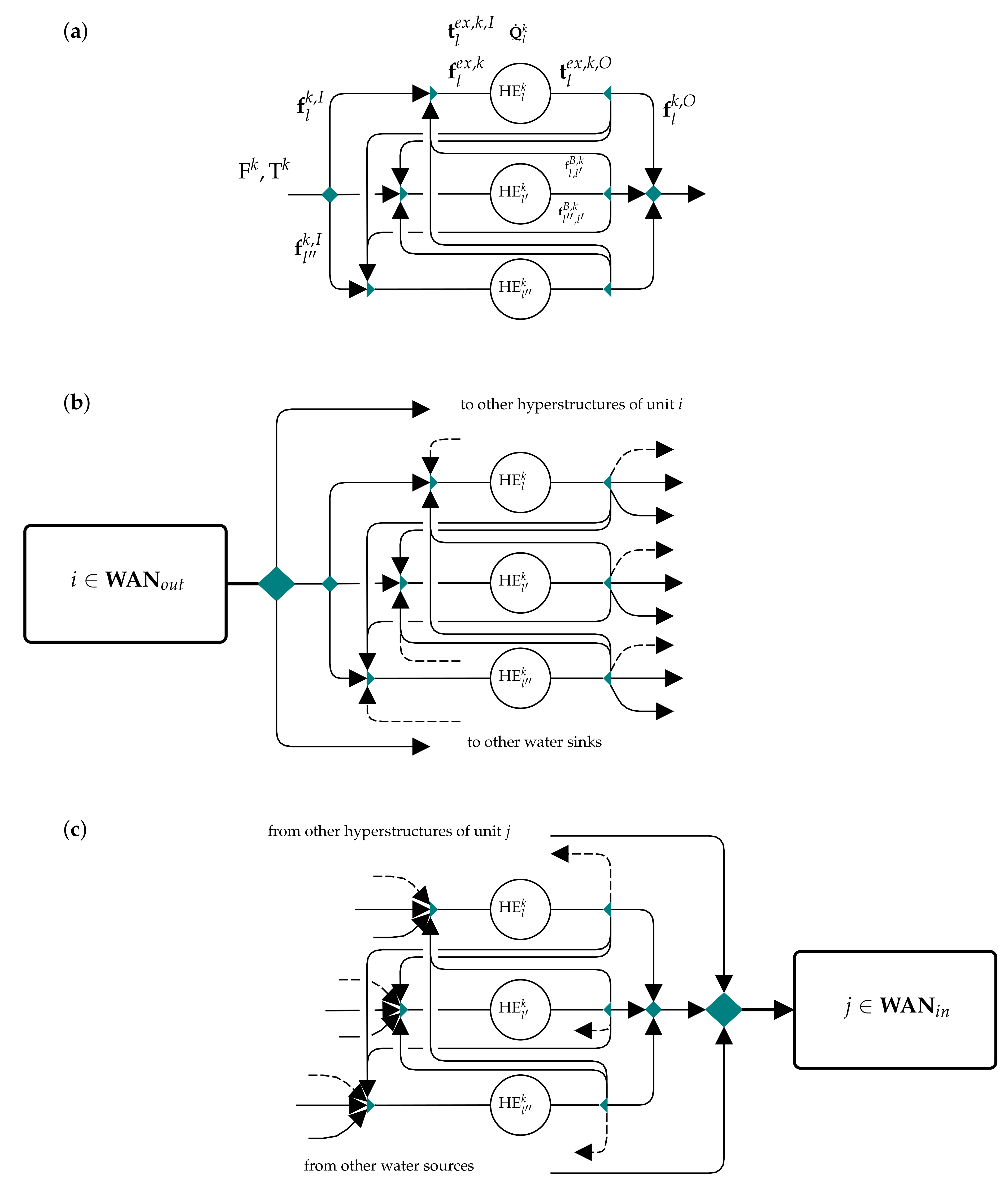
As introduced in Section 1 the overall MINLP formulation of HIWAN is decomposed in three sub-problems denoted P1, P2 and P3. In problem P1, a discretization technique is applied in which any water stream can be heated or cooled from its initial temperature to reach any other temperature in the water network [14]. By assigning binary variables to the existence of each thermal stream, the solution to problem P1 yields the minimum operating cost of the network by selecting potential thermal streams within the water network. This allows cold and hot streams to be selected for both source and sink units. Problem P2 minimizes the number of thermal matches among this set of streams. Appendix A and Appendix B provide the governing equations of problems P1 and P2, respectively. The HIWAN hyperstructure proposed for the third step (Figure 1), and the focus of this paper, is based on the NLP hyperstructure of Floudas and Ciric [31] (Figure 1a) and has been adapted to the HIWAN problem by applying the following modifications:

• Final mixers are removed from superstructures of streams associated with water source units. Hence, the modified superstructure allows for stream splitting from the outlet of any water source unit heat exchanger. (Figure 1b)
• Initial splitters are removed from superstructures of streams associated with water sink units. Hence, the modified superstructure allows for stream mixing at the heat exchanger inlet of sink water units. (Figure 1c)
• Bypass streams are added between different superstructures associated to one source or one sink (shown as dashed arrows in Figure 1b,c). This mimics ${\mathbf{f}}_{l,l^{\prime }}^{B,k}$ in the HEN hyperstructure (Figure 1a), which characterizes the flow from the splitter following the match between k and $l^{\prime }$ to the mixer preceding the match between k and l within the superstructure of stream k.
• As opposed to the HEN hyperstructure for which heat loads of each match (${\dot{\mathbf{Q}}}_l^k$) are fixed at their optimal values from the HLD model, the proposed HIWAN hyperstructure relaxes this constraint; hence, ${\dot{\mathbf{Q}}}_l^k$ can become zero indicating that the match is no longer necessary. For non-water thermal streams (cold or hot), the sum over hot or cold streams, respectively, is fixed to the stream heat load. In essence, ${\dot{\mathbf{Q}}}_l^k$ for non-water thermal streams are allowed to deviate from their optimal values determined by the HLD model.
• An important assumption in the proposed hyperstructure is the value of Heat Recovery Approach Temperature (HRAT) for which problem P1 and problem P2 are solved. This value affects the targeting values of thermal utilities as well as the set of potential thermal streams and their matches; therefore, the model is solved iteratively for several HRATs. The NLP hyperstructure is then solved for Heat Exchanger Minimum Approach Temperature (ΔT_min) values equal to HRAT.
• An initial solution to the HEN hyperstructure model is used as an initialization point for the HIWAN problem.

These modifications produce the following novelties:

• Freshwater and wastewater streams can have hot or cold thermal duties. This addition treats situations in which freshwater cooling or wastewater heating is required.
• In most superstructures proposed in the literature, only one thermal stream is assigned to the outlet of a source water unit operation. As a result, no water stream can be split at the outlet of a heat exchanger for mixing with other streams. This issue is handled in the proposed HIWAN hyperstructure by removing the final mixers of source units. This issue is also treated for sink units by removing their initial splitters.

In order to present the constraints in a coherent way, similar set definitions of Floudas and Ciric [31] have been adapted to represent stream superstructures and matches:

(1)

Set $\mathbf{MA}$ is the set of thermal matches $(k,l)$:

$$\mathbf{MA}=\left\{(k,l)\mid k\in \mathbf{HS}\mathrm{and}l\in \mathbf{CS}\mathrm{and}{\mathbf{y}}_{k,l}^{\mathrm{hld}}=1\right\}$$

(1)

(2)

Set $\mathbf{HCS}$ is the set of all thermal streams:

$$\mathbf{HCS}=\mathbf{HS}\cup \mathbf{CS}$$

(2)

where HS and CS are the sets of hot and cold streams, respectively.

(3)

Set ${\mathbf{SM}}_k$ is the set of streams, $k^{\prime }$, matching with stream $k\in \mathbf{HCS}$ [31], i.e., set of all streams, $k^{\prime }$, so that either of the two matches $(k,k^{\prime })$ or $(k,k^{\prime })$ is in the set of thermal matches, $\mathbf{MA}$:

$$\begin{array}{c}\hfill {\mathbf{SM}}_k=\{k^{\prime }\mid (k\in \mathbf{HS}\wedge k^{\prime }\in \mathbf{CS}\wedge (k,k^{\prime })\in \mathbf{MA})\vee \\ \hfill (k\in \mathbf{CS}\wedge k^{\prime }\in \mathbf{HS}\wedge (k^{\prime },k)\in \mathbf{MA})\}\end{array}$$

(3)

(4)

Set ${\mathbf{SM}}_{i,k}$ is the set of streams matching with stream $k\in {\mathbf{S}}_i$ of water unit $i\in \mathbf{WAN}$, where, ${\mathbf{S}}_i$ is the set of all water thermal streams related to water unit i:

$$\begin{array}{c}\hfill {\mathbf{SM}}_{i,k}=\left\{k^{\prime }\mid i\in \mathbf{WAN}\wedge k\in {\mathbf{S}}_u\wedge k^{\prime }\in {\mathbf{SM}}_k\right\}\end{array}$$

(4)

For mass flow variables, superscripts I, O, and B denote heat exchanger inlet, outlet, and bypass streams, respectively.

3.1. Objective Function

The objective function is the total network investment cost, $C^{inv}$, which is the sum of investment costs over all heat exchangers:

$$\mathbf{P}\mathbf{3}:min{C}^{inv}=\sum _{(i,j)\in \mathbf{MA}}\left\{{\alpha }_1+{\alpha }_2{\left(\frac{{\mathbf{Q}}_{i,j}}{{\mathrm{U}}_{i,j}{\mathbf{LMTD}}_{i,j}}\right)}^{\beta }\right\}=\sum _{(i,j)\in \mathbf{MA}}\left\{{\alpha }_1+{\alpha }_2{\left({\mathbf{A}}_{i,j}\right)}^{\beta }\right\}$$

(5)

where, ${\mathbf{Q}}_{i,j}$ is the heat load of match $(i,j)$ which, as stated before, is not fixed at its optimal value from problem P2 but rather defined as a variable. This makes the objective function non-convex. Parameters ${\alpha }_1$, ${\alpha }_2$, and $\beta$ are fixed, area, and exponential cost parameters for heat exchangers. The ${\mathbf{LMTD}}_{i,j}$ is the logarithmic mean temperature difference of match $(i,j)$ defined as:

$${\mathbf{LMTD}}_{i,j}=\frac{\Delta \mathbf{T}{\mathbf{1}}_{i,j}-\Delta \mathbf{T}{\mathbf{2}}_{i,j}}{ln\frac{\Delta \mathbf{T}{\mathbf{1}}_{i,j}}{\Delta \mathbf{T}{\mathbf{2}}_{i,j}}}$$

(6)

where, $\Delta \mathbf{T}{\mathbf{1}}_{i,j}$ and $\Delta \mathbf{T}{\mathbf{2}}_{i,j}$ are the temperature differences at the two ends of heat exchanger of match $(i,j)$. Equation (6) is simplified using Chen’s approximation [35]:

$${\mathbf{LMTD}}_{i,j}={\left(\Delta \mathbf{T}{\mathbf{1}}_{i,j}·\Delta \mathbf{T}{\mathbf{2}}_{i,j}·\frac{\Delta \mathbf{T}{\mathbf{1}}_{i,j}+\Delta \mathbf{T}{\mathbf{2}}_{i,j}}{2}\right)}^{1/3}$$

(7)

3.2. Constraints

Figure 1 illustrates the basics of the proposed hyperstructure for a water source, a water sink, and a non-water thermal stream which are governed by the equations presented in this sub-section.

3.2.1. Water Network Mass and Energy Balances

(1)

Mass balance at the initial splitter of source unit $i\in {\mathbf{WAN}}_{out}$:

$${\dot{\mathbf{m}}}_i=\sum _{k\in {\mathbf{S}}_i}\sum _{l\in {\mathbf{SM}}_{i,k}}{\dot{\mathbf{m}}}_{i,l}^{k,I}+\sum _{j\in {\mathbf{WAN}}_{in}}\left({\dot{\mathbf{m}}}_{i,j}+\sum _{k\in {\mathbf{S}}_j}\sum _{l\in {\mathbf{SM}}_{j,k}}{\dot{\mathbf{m}}}_{i,j,l}^{k,I}\right)$$

(8)

where, ${\dot{\mathbf{m}}}_i$ is the flow rate of source unit i, ${\dot{\mathbf{m}}}_{i,l}^{k,I}$ is the flow rate from source unit i towards the inlet of heat match $(k,l)$ in the superstructure of stream k, ${\dot{\mathbf{m}}}_{i,j}$ is the flow rate between source unit i and sink unit j, and ${\dot{\mathbf{m}}}_{i,j,l}^{k,I}$ is the flow rate from source unit i towards the inlet of heat match $(k,l)$ in the superstructure of stream k of sink unit j.

(2)

Mass balance at the splitter following a match of source unit $i\in {\mathbf{WAN}}_{out}$ ($k\in {\mathbf{S}}_i$, $l\in {\mathbf{SM}}_{i,k}$):

$${\dot{\mathbf{m}}}_{i,l}^{ex,k}=\sum _{k^{\prime }\in {\mathbf{S}}_i}\sum _{\begin{array}{c}{l}^{\prime }\in {\mathbf{SM}}_{i,k^{\prime }}\\ k\ne k^{\prime }\bigvee l\ne l^{\prime }\end{array}}{\dot{\mathbf{m}}}_{i,l^{\prime },l}^{B,k^{\prime },k}+\sum _{j\in {\mathbf{WAN}}_{in}}\left({\dot{\mathbf{m}}}_{i,l,j}^{k,O}+\sum _{k^{\prime }\in {\mathbf{S}}_j}\sum _{l^{\prime }\in {\mathbf{SM}}_{j,k^{\prime }}}{\dot{\mathbf{m}}}_{i,l,j,l^{\prime }}^{k,O,k^{\prime },I}\right)$$

(9)

where, ${\dot{\mathbf{m}}}_{i,l}^{ex,k}$ is the flow rate through heat exchanger of match $(k,l)$ in the superstructure of stream k of source unit i, ${\dot{\mathbf{m}}}_{i,l^{\prime },l}^{B,k^{\prime },k}$ is the flow rate from the outlet of heat exchanger of match $(k,l)$ in the superstructure of stream k towards the heat exchanger inlet of match $(k^{\prime },l^{\prime })$ in the superstructure of stream $k^{\prime }$ where both heat exchangers belong to source unit i, ${\dot{\mathbf{m}}}_{i,l,j}^{k,O}$ is the flow rate towards sink unit j, and ${\dot{\mathbf{m}}}_{i,l,j,l^{\prime }}^{k,O,k^{\prime },I}$ is the flow rate towards the inlet of heat exchanger of match $(k^{\prime },l^{\prime })$ in the superstructure of sink unit j.

(3)

Mass balance at the mixer preceding a match of source unit $i\in {\mathbf{WAN}}_{out}$ ($k\in {\mathbf{S}}_i$, $l\in {\mathbf{SM}}_{i,k}$):

$${\dot{\mathbf{m}}}_{i,l}^{ex,k}=\sum _{k^{\prime }\in {\mathbf{S}}_i}\sum _{\begin{array}{c}{l}^{\prime }\in {\mathbf{SM}}_{i,k^{\prime }}\\ k\ne k^{\prime }\bigvee l\ne l^{\prime }\end{array}}{\dot{\mathbf{m}}}_{i,l,l^{\prime }}^{B,k,k^{\prime }}+{\dot{\mathbf{m}}}_{i,l}^{k,I}$$

(10)

where, ${\dot{\mathbf{m}}}_{i,l}^{ex,k}$ is the flow rate through heat exchanger of match $(k,l)$ in the superstructure of stream k of source unit i, ${\dot{\mathbf{m}}}_{i,l,l^{\prime }}^{B,k,k^{\prime }}$ is the flow rate from the outlet of heat exchanger of match $(k^{\prime },l^{\prime })$ in the superstructure of stream $k^{\prime }$ towards the heat exchanger inlet of match $(k,l)$ in the superstructure of stream k where both heat exchangers belong to source unit i, and ${\dot{\mathbf{m}}}_{i,l}^{k,I}$ is the flow rate from source unit i towards the inlet of heat match $(k,l)$ in the superstructure of stream k.

(4)

Energy balance at the mixer preceding a match of source unit $i\in {\mathbf{WAN}}_{out}$ ($k\in {\mathbf{S}}_i$, $l\in {\mathbf{SM}}_{i,k}$):

$${\dot{\mathbf{m}}}_{i,l}^{ex,k}·{\mathbf{t}}_{i,l}^{ex,k,I}=\sum _{k^{\prime }\in {\mathbf{S}}_i}\sum _{\begin{array}{c}{l}^{\prime }\in {\mathbf{SM}}_{i,k^{\prime }}\\ k\ne k^{\prime }\bigvee l\ne l^{\prime }\end{array}}{\dot{\mathbf{m}}}_{i,l,l^{\prime }}^{B,k,k^{\prime }}·{\mathbf{t}}_{i,l^{\prime }}^{ex,k^{\prime },O}+{\dot{\mathbf{m}}}_{i,l}^{k,I}·{\mathrm{T}}_i$$

(11)

where ${\mathbf{t}}_{i,l}^{ex,k,I}$ (${\mathbf{t}}_{i,l^{\prime }}^{ex,k^{\prime },O}$) is the temperature at the inlet (outlet) of heat exchanger of match $(k,l)$ ($(k^{\prime },l^{\prime })$) in the superstructure of stream k($k^{\prime }$), and ${\mathrm{T}}_i$ is the temperature of source unit i.

(5)

Mass balance at the final mixer of sink unit $j\in {\mathbf{WAN}}_{in}$:

$${\dot{\mathbf{m}}}_j=\sum _{k\in {\mathbf{S}}_j}\sum _{l\in {\mathbf{SM}}_{j,k}}{\dot{\mathbf{m}}}_{j,l}^{k,O}+\sum _{i\in {\mathbf{WAN}}_{out}}\left({\dot{\mathbf{m}}}_{i,j}+\sum _{k\in {\mathbf{S}}_i}\sum _{l\in {\mathbf{SM}}_{i,k}}{\dot{\mathbf{m}}}_{i,l,j}^{k,O}\right)$$

(12)

where, ${\dot{\mathbf{m}}}_j$ is the flow rate of sink unit j, ${\dot{\mathbf{m}}}_{j,l}^{k,O}$ is the flow rate from the outlet of heat match $(k,l)$ in the superstructure of stream k towards sink unit j, ${\dot{\mathbf{m}}}_{i,j}$ is the flow rate between source unit i and sink unit j, and ${\dot{\mathbf{m}}}_{i,l,j}^{k,O}$ is the flow rate from the outlet of heat match $(k,l)$ in the superstructure of stream k of source unit i towards sink unit j.

(6)

Mass balance at the splitter following a match of sink unit $j\in {\mathbf{WAN}}_{out}$ ($k\in {\mathbf{S}}_j$, $l\in {\mathbf{SM}}_{j,k}$):

$${\dot{\mathbf{m}}}_{j,l}^{ex,k}=\sum _{k^{\prime }\in {\mathbf{S}}_j}\sum _{\begin{array}{c}{l}^{\prime }\in {\mathbf{SM}}_{j,k^{\prime }}\\ k\ne k^{\prime }\bigvee l\ne l^{\prime }\end{array}}{\dot{\mathbf{m}}}_{j,l^{\prime },l}^{B,k^{\prime },k}+{\dot{\mathbf{m}}}_{j,l}^{k,O}$$

(13)

where, ${\dot{\mathbf{m}}}_{j,l}^{ex,k}$ is the flow rate through heat exchanger of match $(k,l)$ in the superstructure of stream k of sink unit j and ${\dot{\mathbf{m}}}_{j,l^{\prime },l}^{B,k^{\prime },k}$ is the flow rate from the outlet of heat exchanger of match $(k,l)$ in the superstructure of stream k towards the heat exchanger inlet of match $(k^{\prime },l^{\prime })$ in the superstructure of stream $k^{\prime }$ where both heat exchangers belong to sink unit j.

(7)

Mass balance at the mixer preceding a match of sink unit $j\in {\mathbf{WAN}}_{out}$ ($k\in {\mathbf{S}}_j$, $l\in {\mathbf{SM}}_{j,k}$):

$${\dot{\mathbf{m}}}_{j,l}^{ex,k}=\sum _{k^{\prime }\in {\mathbf{S}}_j}\sum _{\begin{array}{c}{l}^{\prime }\in {\mathbf{SM}}_{j,k^{\prime }}\\ k\ne k^{\prime }\bigvee l\ne l^{\prime }\end{array}}{\dot{\mathbf{m}}}_{j,l,l^{\prime }}^{B,k,k^{\prime }}+\sum _{i\in {\mathbf{WAN}}_{out}}\left({\dot{\mathbf{m}}}_{i,j,l}^{k,I}+\sum _{k^{\prime }\in {\mathbf{S}}_i}\sum _{l^{\prime }\in {\mathbf{SM}}_{i,k^{\prime }}}{\dot{\mathbf{m}}}_{i,l^{\prime },j,l}^{k^{\prime },O,k,I}\right)$$

(14)

where, ${\dot{\mathbf{m}}}_{j,l,l^{\prime }}^{B,k,k^{\prime }}$ is the flow rate from the outlet of heat exchanger of match $(k^{\prime },l^{\prime })$ in the superstructure of stream $k^{\prime }$ towards the heat exchanger inlet of match $(k,l)$ in the superstructure of stream k where both heat exchangers belong to sink unit j, ${\dot{\mathbf{m}}}_{i,j,l}^{k,I}$ is the flow rate from source unit i towards the inlet of heat match $(k,l)$ in the superstructure of stream k of sink unit j, and ${\dot{\mathbf{m}}}_{i,l^{\prime },j,l}^{k^{\prime },O,k,I}$ is the flow rate from the outlet of heat match $(k^{\prime },l^{\prime })$ in the superstructure of stream $k^{\prime }$ of source unit i towards the inlet of heat exchanger of match $(k,l)$ in the superstructure of stream k of sink unit j.

(8)

Energy balance at the mixer preceding a match of sink unit $j\in {\mathbf{WAN}}_{out}$ ($k\in {\mathbf{S}}_j$, $l\in {\mathbf{SM}}_{j,k}$):

$$\begin{array}{cc}\hfill {\dot{\mathbf{m}}}_{j,l}^{ex,k}·{\mathbf{t}}_{j,l}^{ex,k,I}& =\sum _{k^{\prime }\in {\mathbf{S}}_j}\sum _{\begin{array}{c}{l}^{\prime }\in {\mathbf{SM}}_{j,k^{\prime }}\\ k\ne k^{\prime }\bigvee l\ne l^{\prime }\end{array}}{\dot{\mathbf{m}}}_{j,l,l^{\prime }}^{B,k,k^{\prime }}·{\mathbf{t}}_{j,l^{\prime }}^{ex,k^{\prime },O}\hfill \\ & +\sum _{i\in {\mathbf{WAN}}_{out}}\left({\dot{\mathbf{m}}}_{i,j,l}^{k,I}·{\mathrm{T}}_i+\sum _{k^{\prime }\in {\mathbf{S}}_i}\sum _{l^{\prime }\in {\mathbf{SM}}_{i,k^{\prime }}}{\dot{\mathbf{m}}}_{i,l^{\prime },j,l}^{k^{\prime },O,k,I}·{\mathbf{t}}_{i,l^{\prime }}^{ex,k^{\prime },O}\right)\hfill \end{array}$$

(15)

where ${\mathbf{t}}_{j,l}^{ex,k,I}$ (${\mathbf{t}}_{j,l^{\prime }}^{ex,k^{\prime },O}$) is the temperature at the inlet (outlet) of heat exchanger of match $(k,l)$ $(k^{\prime },l^{\prime })$ in the superstructure of stream k ($k^{\prime }$) and ${\mathrm{T}}_j$ is the temperature of sink unit j.

(9)

Energy balance in matches of stream $k\in {\mathbf{S}}_u$ of water unit $u\in \mathbf{WAN}$:

$${\mathbf{Q}}_{k,l}={\dot{\mathbf{m}}}_{i,l}^{ex,k}{\mathrm{c}}_p|{\mathbf{t}}_{i,l}^{ex,k,O}-{\mathbf{t}}_{i,l}^{ex,k,I}|$$

(16)

3.2.2. Contamination Constraints

(10)

Contamination equality constraint at the final mixer of sink unit $j\in {\mathbf{WAN}}_{in}$ for contaminant $k\in \mathbf{C}$:

$$\begin{array}{cc}\hfill {\dot{\mathbf{m}}}_j·{\mathbf{c}}_j^{k,in}& =\sum _{i\in {\mathbf{WAN}}_{out}}({\dot{\mathbf{m}}}_{i,j}+\sum _{k\in {\mathbf{S}}_i}\sum _{l\in {\mathbf{SM}}_{i,k}}{\dot{\mathbf{m}}}_{i,l,j}^{k,O}\hfill \\ & +\sum _{k^{\prime }\in {\mathbf{S}}_j}\sum _{l^{\prime }\in {\mathbf{SM}}_{j,k^{\prime }}}\left({\dot{\mathbf{m}}}_{i,j,l^{\prime }}^{k^{\prime },I}+\sum _{k\in {\mathbf{S}}_i}\sum _{l\in {\mathbf{SM}}_{i,k}}{\dot{\mathbf{m}}}_{i,l,j,l^{\prime }}^{k,O,k^{\prime },I}\right))·{\mathbf{c}}_i^{k,out}\hfill \end{array}$$

(17)

where ${\mathbf{c}}_j^{k,in}$ is the contamination level of contaminant k at the inlet of sink unit j, and ${\mathbf{c}}_i^{k,out}$ is the contamination level of contaminant k at the outlet of source unit i.

(11)

Contamination at the inlet of unit $j\in {\mathbf{WAN}}_{in}$ should be less than a maximum allowed value:

$${\mathbf{c}}_j^{k,in}-{\mathrm{c}}_j^{k,in,max}\le 0$$

(18)

(12)

Mass transfer equality constraint for mass transfer unit $u\in \mathbf{WAN}$:

$$\sum _{j\in {\mathbf{WAN}}_{u,in}}{\dot{\mathbf{m}}}_j·{\mathbf{c}}_j^{k,in}+{\mathrm{L}}_u-\sum _{i\in {\mathbf{WAN}}_{u,out}}{\dot{\mathbf{m}}}_i·{\mathbf{c}}_i^{k,out}=0$$

(19)

where ${\dot{\mathbf{m}}}_j={\dot{\mathbf{m}}}_i$ and ${\mathbf{WAN}}_{u,in}$ (${\mathbf{WAN}}_{u,out}$) is the set of sinks (sources) associated to mass transfer unit u.

(13)

Outlet contamination of unit $i\in {\mathbf{WAN}}_{out}$ should be less than a maximum allowed value:

$${\mathbf{c}}_i^{k,out}-{\mathrm{c}}_i^{k,out,max}\le 0$$

(20)

3.2.3. Mass and Energy Balances in Non-Water Streams Superstructure

The mass and energy balances of non-water thermal streams follow the same constraints of the HEN synthesis problem of Floudas and Ciric [31] (Figure 1a introduces the full set of related variables and parameters):

(14)

Mass balance at the initial splitter of stream $k\in \mathbf{HCS}$:

$${\mathrm{F}}^k-\sum _{l\in {\mathbf{SM}}_k}{\mathbf{f}}_l^{k,I}=0$$

(21)

where, ${\mathrm{F}}^k$ is the heat capacity flow rate of stream k and ${\mathbf{f}}_l^{k,I}$ is the heat capacity flow rate of stream k towards the inlet of heat exchanger of match $(k,l)/(l,k)$ in the superstructure of stream k.

(15)

Mass balance at the mixer preceding a heat exchanger of stream $k\in \mathbf{HCS}$:

$${\mathbf{f}}_l^{ex,k}-{\mathbf{f}}_l^{k,I}-\sum _{\begin{array}{c}{l}^{\prime }\in {\mathbf{SM}}_k,l\ne l^{\prime }\end{array}}{\mathbf{f}}_{l,l^{\prime }}^{B,k}=0\forall l\in {\mathbf{SM}}_k$$

(22)

(16)

Mass balance at the splitter following a heat exchange match of stream $k\in \mathbf{HCS}$:

$${\mathbf{f}}_l^{ex,k}-{\mathbf{f}}_l^{k,O}-\sum _{\begin{array}{c}{l}^{\prime }\in {\mathbf{SM}}_k,l\ne l^{\prime }\end{array}}{\mathbf{f}}_{l^{\prime },l}^{B,k}=0\forall l\in {\mathbf{SM}}_k$$

(23)

(17)

Energy balance at the mixer preceding a heat exchange match of stream $k\in \mathbf{HCS}$:

$${\mathbf{f}}_l^{ex,k}·{\mathbf{t}}_l^{ex,k,I}-{\mathbf{f}}_l^{k,I}·{\mathrm{T}}_k-\sum _{\begin{array}{c}{l}^{\prime }\in {\mathbf{SM}}_k,l\ne l^{\prime }\end{array}}{\mathbf{f}}_{l,l^{\prime }}^{B,k}·{\mathbf{t}}_{l^{\prime }}^{ex,k,O}=0\forall l\in {\mathbf{SM}}_k$$

(24)

(18)

Energy balance of heat exchange match $(k,l)\in \mathbf{MA}$ (as mentioned previously, heat load is defined as a variable in the HIWAN model):

$$\begin{array}{c}\hfill {\mathbf{Q}}_{k,l}={\mathbf{f}}_l^{ex,k}·({\mathbf{t}}_l^{ex,k,I}-{\mathbf{t}}_l^{ex,k,O})\\ \hfill {\mathbf{Q}}_{k,l}={\mathbf{f}}_k^{ex,l}·({\mathbf{t}}_k^{ex,l,O}-{\mathbf{t}}_k^{ex,l,I})\end{array}$$

(25)

(19)

Energy balance of hot and cold non-water thermal streams:

$${\mathrm{Q}}_k=\sum _{l\in {\mathbf{SM}}_k}{\mathbf{Q}}_{k,l}\forall k\in \mathbf{HCS}|k\notin \bigcup _{u\in \mathbf{WAN}}{\mathbf{S}}_u$$

(26)

This constraint holds for all thermal streams $k\in \mathbf{HCS}$ that do not belong to any water unit operation. ${\mathrm{Q}}_k$ is the heat load of non-water thermal stream k.

3.2.4. Temperature Difference Constraints

(20)

Temperature difference at the two ends of heat exchanger $(k,l)\in \mathbf{MA}$:

$$\begin{array}{c}\hfill \Delta \mathbf{T}{\mathbf{1}}_{k,l}={\mathbf{t}}_l^{ex,k,I}-{\mathbf{t}}_k^{ex,l,O}\Delta \mathbf{T}{\mathbf{2}}_{k,l}={\mathbf{t}}_l^{ex,k,O}-{\mathbf{t}}_k^{ex,l,I}\end{array}$$

(27)

(21)

Minimum approach temperature difference:

$$\begin{array}{c}\hfill \Delta \mathbf{T}{\mathbf{1}}_{k,l}\ge \Delta {\mathrm{T}}_{min}=\mathrm{HRAT}\Delta \mathbf{T}{\mathbf{2}}_{k,l}\ge \Delta {\mathrm{T}}_{min}=\mathrm{HRAT}\end{array}$$

(28)

4. Solution Strategy

As discussed in Section 3, the HIWAN synthesis problem is decomposed into three sub-problems:

Step 1—Targeting Model (problem P1): At this step, a value of HRAT is assumed for water thermal streams. For non-water thermal streams, this value depends on the nature of the stream and problem requirements or can be assigned based on general assumptions. A solution of this model provides the utility targets of the HIWAN synthesis problem and a list of water thermal streams with their corresponding heat loads. Moreover, a water allocation network will be generated satisfying the temperature and contamination constraints (Appendix A) [14].

Step 2—Heat Load Distribution Model (problem P2): The input of this model is the list of thermal streams with their corresponding heat loads from Step 1. A solution of this model provides a set of potential thermal matches with their corresponding heat loads which exhibits the minimum number of heat exchangers. Several solutions may exist with the minimum number of heat exchangers. This is addressed in the proposed solution strategy by applying Integer-Cut Constraints (ICCs). The water allocation network is fixed at its solution from Step 1 (Equation (A2)) for this stage.

Step 3—HIWAN Hyperstructure Model (problem P3-NLP): The model takes the water data and utility targets from Step 1, while the thermal matches and their heat loads are provided from Step 2. Since the water allocation network superstructure is embedded in this model, the water allocation network from Step 1 can be changed but provides an initial, feasible solution. Additionally, heat loads of thermal matches are relaxed at this step; hence, heat exchanger flows can reach zero, indicating that the optimized water network flows and temperatures do not require the existence of this exchanger. The variables of this problem, i.e., flows, temperatures, and heat loads of all heat exchangers, are initialized by solving the HEN hyperstructure of Floudas and Ciric [31] (model P3${}^{\mathrm{init}}$-NLP). It should be highlighted that a solution to P3${}^{\mathrm{init}}$-NLP is a feasible solution to the HIWAN synthesis problem.

Solving the above-mentioned steps in sequence provides, at most, two solutions to the HIWAN synthesis problem: the solutions of P3${}^{\mathrm{init}}$-NLP and P3-NLP. Compared to simultaneous approaches, sequential approaches are easier to solve due to reduced problem size at each step. Nevertheless, similar drawbacks observed for sequential solution strategies that are applied in HEN synthesis problems [31] are also valid in this case:

• The trade-off between operating cost and investment cost (i.e., number of matches and area) cannot be fully captured in sequential solution strategies.
• The nature of the HIWAN synthesis problem is non-convex and hence global optimality cannot be guaranteed.
• Problem P2-MILP provides only one feasible solution providing the minimum number of heat exchangers. Therefore, sequentially minimizing the number of heat exchangers followed by HEN synthesis does not guarantee a HIWAN exhibiting the lowest total cost.

To address these drawbacks, an iterative sequential solution strategy is proposed by applying an integer cut constraint on problems P1 and P2. In addition, the problem is solved for different values of HRAT to address the pinch point decomposition of temperature intervals and to get different utility targets with the goal of achieving lower investment costs. Applying integer cut constraints at Steps 1 and 2 provides a double benefit:

►

By assuming the overall synthesis problem encompasses all water thermal streams and states (hot and cold), problems P1 and P2 limit the search space to a specific region, i.e., a specific set of potential thermal streams with their corresponding states and a specific set of thermal matches. This allows for a smaller problem size at Step 3 and hence provides guidance towards a good solution. Applying an integer cut constraint generates several “reduced-size” problems and increases the opportunities for identifying good solutions.

►

By applying, for example, $N_{icc}^{\mathbf{P}\mathbf{1}}$ and $N_{icc}^{\mathbf{P}\mathbf{2}}$ integer cuts at Steps 1 and 2, respectively, $(N_{icc}^{\mathbf{P}\mathbf{1}}+1)(N_{icc}^{\mathbf{P}\mathbf{2}}+1)$ solutions to the HIWAN synthesis problem can be generated. These solutions can be ranked based on different key performance indicators and thus guide the decision-making process toward a “good” solution.

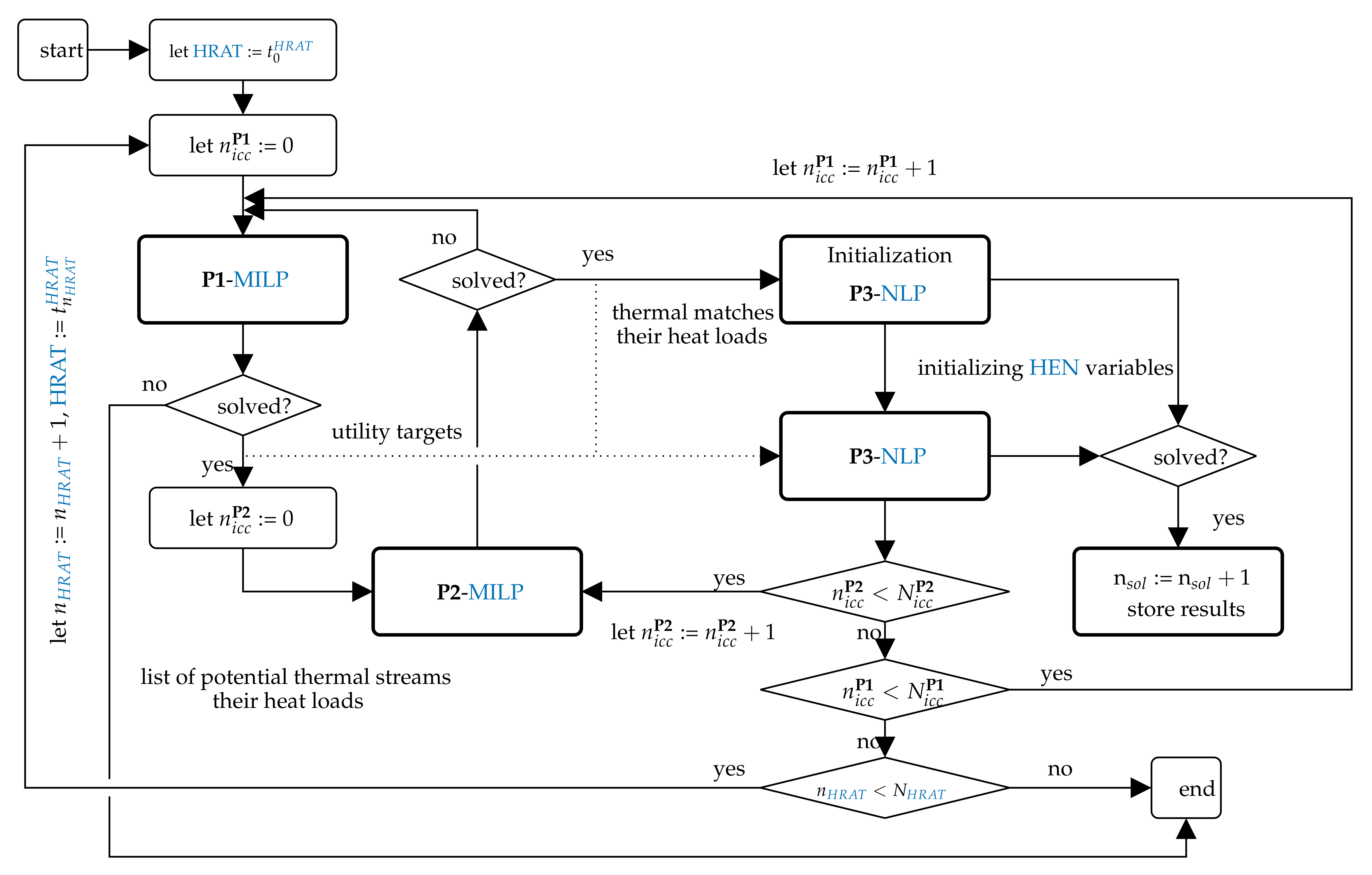
This approach can be regarded as iteratively optimizing the overall MINLP model within different regions of the global search space (as imposed by the formulations of problems P1 and P2 at each iteration). Figure 2 illustrates the proposed solution strategy. It should be noted that, similar to other methodologies, the choice of solver and its options affects the path toward a solution.

5. Illustrative Example

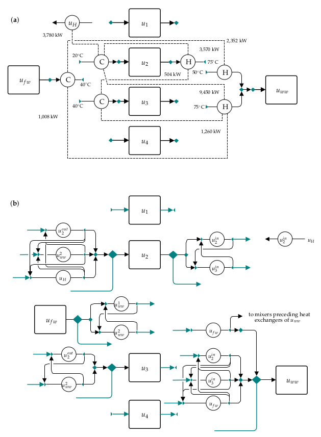
The four-water-unit-operation, single-contaminant case study of Savulescu and Smith [36] was selected to demonstrate the generation of the proposed HIWAN hyperstructure. First, problem P1 is solved providing minimum freshwater, hot, and cold utility consumption of 90 kg/s, 3780 kW, and 0 kW, respectively. Problem P1 also provides a feasible water allocation scheme. Given the list of thermal streams, problem P2 is solved which results in seven matches (Figure 3a). There are several solutions to problem P2 with an objective value of seven. For the sake of illustration, the fourth solution (by applying three integer cuts) is shown in Figure 3a and will be discussed hereafter. The CPLEX solver [37] was used for both MILP problems (

Table 1. Solver options for the illustrative example.

Stage	Options	Value	Description
AMPL [39]	presolve_eps	10${}^{-5}$	maximum difference between lower and upper bounds in constraint violations
P1-MILP	mipgap	10${}^{-4}$	relative improvement in integer solution below which optimization is terminated
	integrality	10${}^{-10}$	a variable is considered to have an integral value if it lies within that of an integer
P2-MILP	mipgap	10${}^{-4}$
	integrality	10${}^{-4}$
P3-HEN-NLP [31]	feas_tol	10${}^{-5}$	satisfying upper and lower bounds of variables and linear constraints
P3-NLP	feas_tol	10${}^{-4}$

). Figure 3b presents the HIWAN hyperstructure constructed based on the results provided in Figure 3a. The HIWAN hyperstructure generation follows the same approach as the HEN hyperstructure [31], as shown in Figure 3a. The inlet of unit $u_2$ has one cold thermal stream which has one match with hot utility $u_H$, one match with wastewater unit $u_{ww}$ and one match with its outlet; hence, one superstructure with three matches is defined for this stream. The Wastewater unit $u_{ww}$ has two cold streams with one and three matches, respectively. This results in a hyperstructure consisting of two stream superstructures as illustrated in Figure 3b. As presented in Figure 1 for the proposed hyperstructure, mass flows can be split from source unit heat exchanger outlets and mixed at sink unit heat exchanger inlets. This has been illustrated in Figure 3b with thicker, colored arrows.

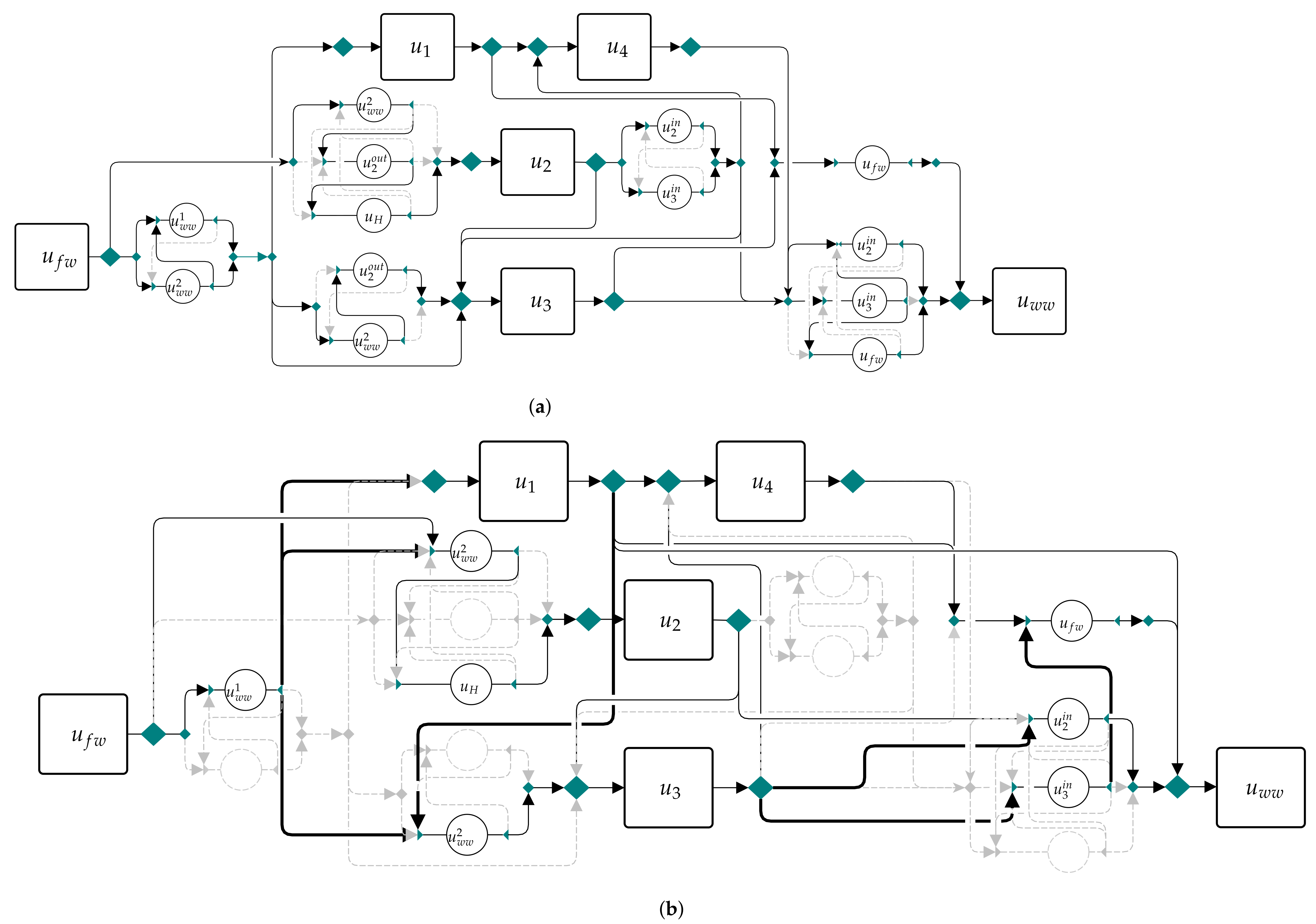
HIWAN synthesis is solved for problem P3 as well as for the HEN model of Floudas and Ciric [31]. SNOPT solver [38] is used to solve both models (Table 1). Its algorithm is based on sequential quadratic programming (SQP) and its solutions are locally optimal. It should be noted that problem P3 is non-convex and hence the global optimality of the solutions cannot be guaranteed. The solution of the NLP hyperstructure of Floudas and Ciric [31] is shown in Figure 4a. Since this solution is based on the results of HLD, all seven heat exchangers are active. The area of heat exchangers 3 (55.4 m${}^2$) and 7 (196.4 m${}^2$) are relatively small compared to the others (

Table 2. Comparison of two approaches based on key HEN indicators ${}^{\left(1\right)}$.

${\mathrm{y}}_{\mathit{i},\mathit{j}}$		${\mathrm{t}}_{\mathit{j}}^{\mathit{ex},\mathit{i},\mathit{I}}$ [${}^{\circ }$C]	${\mathrm{t}}_{\mathit{j}}^{\mathit{ex},\mathit{i},\mathit{O}}$ [${}^{\circ }$C]	${\mathrm{t}}_{\mathit{i}}^{\mathit{ex},\mathit{j},\mathit{I}}$ [${}^{\circ }$C]	${\mathrm{t}}_{\mathit{i}}^{\mathit{ex},\mathit{j},\mathit{O}}$ [${}^{\circ }$C]	${\mathbf{LMTD}}_{\mathit{i},\mathit{j}}$ [${}^{\circ }$C]	${\mathbf{Q}}_{\mathit{i},\mathit{j}}$ [kW]	${\mathbf{A}}_{\mathit{i},\mathit{j}}$ [m${}^2$]	${\mathbf{C}}_{\mathit{i},\mathit{j}}^{\mathit{inv}}$ [USD/yr]
1	$u_H$-$u_2^{in}$ ${}^{\left(2\right)}$	120.00	120.00	81.96	99.96	28.1	3780.0	269.2	42,453
2	$u_2^{out}$-$u_2^{in}$	100.00 (-)	74.61 (-)	64.62 (-)	81.62 (-)	13.8 (-)	3570.0 (-)	518.9 (-)	59,078 (-)
3	$u_2^{out}$-$u_3^{in}$	100.00 (-)	77.70 (-)	64.96 (-)	74.96 (-)	18.2 (-)	504.0 (-)	55.4 (-)	21,342 (-)
4	$u_{ww}^1$-$u_{fw}$	50.00	30.00	20.00	40.00	10.0	2352.0	470.4	56,157
		(50.24)	(30.00)	(20.00)	(40.03)	(10.1)	(3371.4)	(667.3)	(67,398)
5	$u_{ww}^2$-$u_2^{in}$	75.00	30.00	20.00	65.00	10.0	9450.0	1890.0	118,932
		(91.92)	(30.00)	(20.00)	(81.93)	(10.0)	(13,004.7)	(2602.2)	(142,397)
6	$u_{ww}^2$-$u_3^{in}$	75.00	50.52	40.00	65.00	10.3	1260.0	245.7	40,613
		(75.01)	(55.24)	(40.00)	(57.86)	(16.2)	(1782.5)	(220.3)	(38,550)
7	$u_{ww}^2$-$u_{fw}$	50.20 (-)	30.20 (-)	20.00 (-)	39.87 (-)	10.3 (-)	1008.0 (-)	196.4 (-)	36,514 (-)
	Total							3645.9	375,089
								(3759.0)	(290,799)

⁽¹⁾ i and j represent hot and cold streams, respectively. Values in parentheses are results of HIWAN hyperstructure. ⁽²⁾ Same values in both cases.

). This approach, however, does not account for the possibility of stream mixing and splitting. The HIWAN hyperstructure addresses these possibilities by embedding the water allocation network within the HEN hyperstructure. Figure 4b presents the results of the proposed hyperstructure. By considering additional possibilities for stream mixing and splitting, hence increased possibility of non-isothermal mixing, three out of the seven targeted heat exchangers are determined not to be required. The flows in bold illustrate the new possibilities embedded in the proposed HIWAN hyperstructure. Consequently the HEN cost is reduced by 22.47 % (290,799 compared to 375,089 kUSD/yr). Table 2 provides the temperatures, flows and heat loads associated to heat exchangers in both cases.

6. Validation and Discussion

Two test cases from the literature were selected to validate the mathematical formulation and the proposed iterative sequential solution strategy. The cost data are presented in

Table 3. Economic and operating parameters for all test cases [4].

Parameters	Units	Values for Cases Studies
		Test Case I	Test Case II
			(Simplified Kraft)
Cost of freshwater	USD/t	0.375	0.1525
Cost of cold utility	USD/kWyr	189	18.568
Cost of hot utility (steam, 120 ${}^{\circ }$C)	USD/kWyr	377	140.16
Temperatures of cold utility	${}^{\circ }$C	10 → 20	10 → 35
Heat-transfer coefficient	kW/m${}^2$K	1	1
Operating hours	hr/yr	8000	8322
Interest rate	%	8	8
Plant lifetime	yr	25	25
Temperature of freshwater	${}^{\circ }$C	20	10
Temperature of wastewater	${}^{\circ }$C	30	30
Specific heat capacity of water	kJ/kg.K	4.2	4.2
ΔTmin of hot and cold utilities	${}^{\circ }$C	10	10
Heat exchanger cost coefficients (Equation (5)) [4]
${\alpha }_1$	USD/yr	8000
${\alpha }_2$	USD/yr/m${}^{0.6}$	1200
$\beta$	-	0.6

. The maximum number of integer cuts was limited to 50, though one sub-problem (P1 or P2) may become infeasible before reaching its respective limit, at which point the algorithm terminates the corresponding integer cut loop. In combination with the application of integer cut constraints, small minimum sizes were introduced for all water units in problem P1 (0.05 kg/s). Similarly, for problem P2, the minimum allowed heat exchange between hot stream i and cold stream j in pinch interval l is set at a small positive number (${\mathrm{Q}}_{i,j,l}^{min}=0.1$ kW in Equation (A6)). These two additions prevent generation of multiple identical solutions. Furthermore, to investigate the trade-off between investment cost and operating cost, the HRAT in problem P1 was varied between 1 ${}^{\circ }$C and 10 ${}^{\circ }$C with step of 1 ${}^{\circ }$C (N${}_{\mathrm{H}\mathrm{R}\mathrm{A}\mathrm{T}}$ = 10). These values are passed to problem P3 to be used as the value of ΔT_min. Test case I is a threshold problem and hence the value of HRAT does not affect the utility consumption. This, however, becomes a decisive factor for test case II where both hot and cold utilities are required. In this section, only solutions of the HIWAN hyperstructure are presented. A parallel coordinate visualization tool is used to illustrate all solutions and selected key performance indicators. These key performance indicators (KPI)s are listed here:

• Resource indicators: freshwater and thermal utility consumption, ${\dot{\mathbf{m}}}_{fw}$, ${\dot{\mathbf{Q}}}_u^H$, ${\dot{\mathbf{Q}}}_u^C$;
• Network indicators: N${}_s^{th}$ (number of thermal streams), N${}_{\mathrm{H}\mathrm{E}}$ (number of heat exchangers), A${}_{\mathrm{H}\mathrm{E}\mathrm{N}}^{total}$ (total area of heat exchangers), N${}_{mixer}$ (number of mixing points), N${}_{mixer}^{NIM}$ (number of non-isothermal mixing points), N${}_s^m$ (number of mass streams in the water network), and Q${}_{\mathrm{H}\mathrm{E}\mathrm{N}}^{total}$ (total heat load of all heat exchangers);
• Economic indicators: C${}^{\mathrm{H}\mathrm{E}\mathrm{N}}$ (HEN cost) and C${}^{\mathrm{T}\mathrm{A}\mathrm{C}}$ (total annualized cost).

It should be noted that test case I was intentionally designed by the scientific community to validate their mathematical formulations and solution strategies. Due to the complexity of solving non-convex MINLP problems that arise in HIWAN synthesis, and solver tendency toward local optimality in such problems, it can be argued that these test cases are not easily solved without carefully manipulating solvers and their intrinsic options to reach a single, ´´good” solution. Thus, the main goal and contribution of the proposed solution strategy in this work is to solve the HIWAN problem by first reducing the search space, then generating many solutions to the problem. To this end, many solutions can be generated for problem P3 which can be seen as approaching an optimal point from different starting points (solutions of problems P1 and P2).

6.1. Test Case I—Single-Contaminant Problem

This test case in its optimal configuration [14,40,41] exhibits 90 kg/s of freshwater consumption and 3780 kW of hot utility consumption (minimum targets, 2397.0 kUSD/yr in operating cost).

Table A1. Assumption and solver options for test cases I and II.

Solver Option	Value (I)	Value (II)	Description (Mainly from Respective Solver’s Manual)
AMPL
reset_initial_guesses	1	1	Reset variables to their initial values between different calls to solve command (all steps)
presolve_eps	variable	variable	Maximum difference between lower and upper bounds in constraint violations
			P1: 10${}^{-6}$ (test case I), 10${}^{-4}$ (test case II) and 10${}^{-5}$ for all others
presolve	1	1	Simplifying problem prior to the solver by fixing variables and dropping redundant constraints (all steps)
P1 (CPLEX)
mipgap	10${}^{-4}$	10${}^{-5}$	Relative tolerance for optimizing integer variables: stop if abs((best bound) − (best integer)) < mipgap * (1 + abs(best bound)).
integrality	10${}^{-10}$	10${}^{-4}$	Amount by which an integer variable can differ from the nearest integer and still be considered feasible.
P2 (CPLEX)
mipgap	10${}^{-7}$	10${}^{-5}$	See above
integrality	10${}^{-10}$	10${}^{-8}$	See above
P3 (initialization) (SNOPT)
▹ Problem P3 is solved by minimizing the sum of flows between heat exchangers
meminc	1	1	Increment to minimum memory allocation
iterations	10${}^6$	10${}^6$	Minor iteration limit
feas_tol	10${}^{-6}$	10${}^{-4}$	Minor feasibility tolerance for all variables and linear constraints
P3 and P3 HIWAN hyperstructure (SNOPT)
meminc = 1 iterations = 10${}^6$ feas_tol = 10${}^{-4}$ (see above)

HRAT = ΔT_min for each iteration. Enthalpy values of thermal stream are rounded for HEN design to 10${}^{-6}$. Optimality gap of heat balance constraints (HIWAN) at mixing points is set at 0.01%. For problem P1, sum of mass exchanges is added to the objective function (Equation (A1)) to reduce the number of mass exchanges while minimizing the total cost.

provides the assumptions and solver options for this test case. Out of 26,010 potential solutions, 6462 solutions exist to problem P2—this arises from the fact that problem P1 converged for all integer cuts, while problem P2 was found to be infeasible for low HRAT values after relatively few integer cuts. 3611 solutions exist to problem P3. They exhibit a wide spectrum of solutions with HEN cost (the objective function in problem P3) ranging from 255.1 kUSD/yr (the minimum value within the literature [5]) to 660.9 kUSD/yr. Among these, 3506 solutions exhibit HEN cost in the range reported in the literature [5] (the maximum observed cost is 413.0 kUSD/yr). To visualize this set of solutions, several filters were imposed to further reduce the number of solutions:

• ${\mathrm{C}}^{\mathrm{H}\mathrm{E}\mathrm{N}}\le$ 300 kUSD/yr;
• N${}_s^m$ ≤ 15, maximum value reported in the literature for this test case [5];
• N${}_{mixer}$ ≤ 13, maximum value reported in the literature for this test case [5];
• N${}_{mixer}^{NIM}$ ≤ 10, maximum value reported in the literature for this test case in [5];

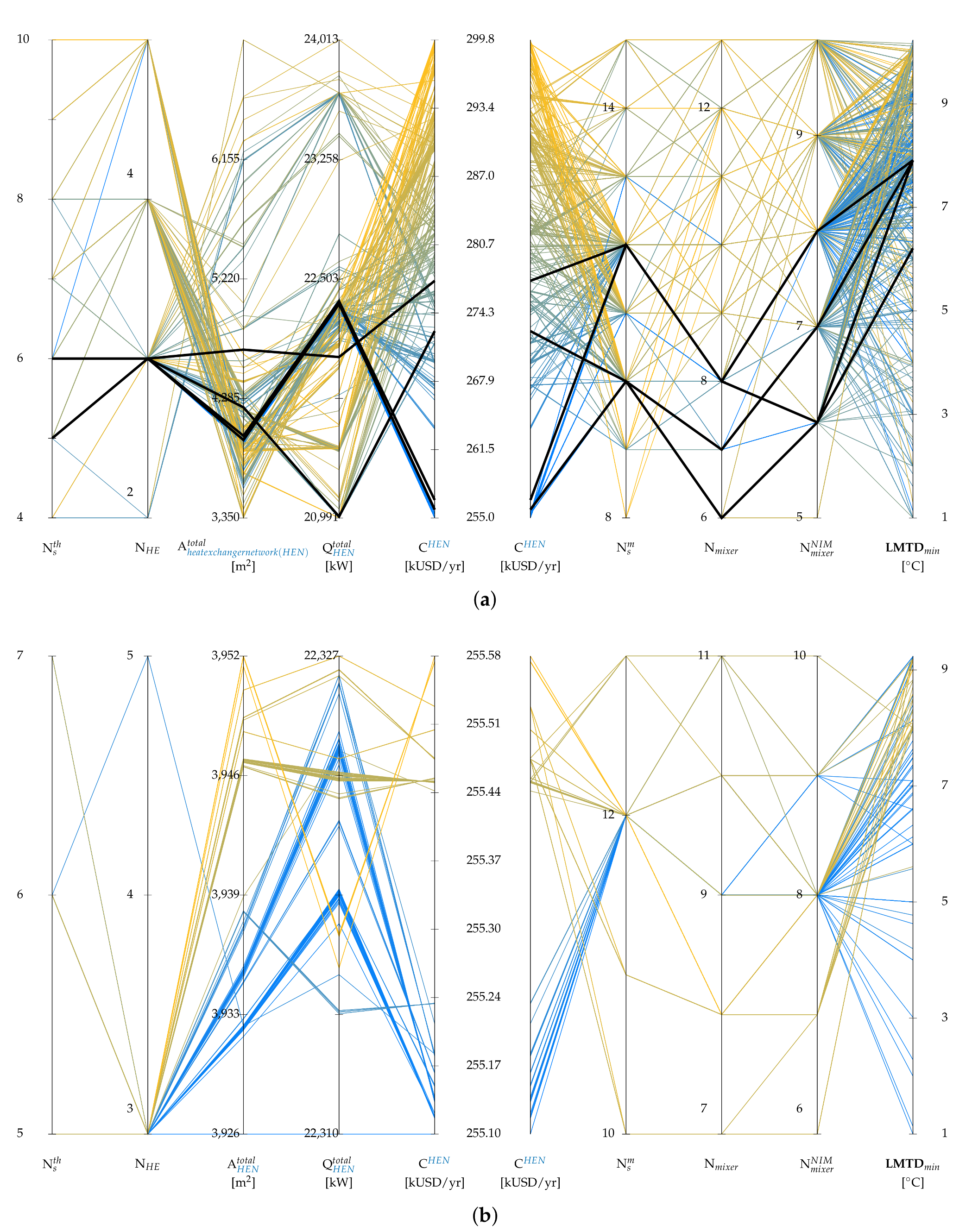
Figure 5 presents 2247 solutions which remain after filtering (the color spectrum is based on HEN cost). Selected results from the literature [5] with HEN cost lower than 300 kUSD/yr are also plotted in this figure in black bold. The number of heat exchangers (N${}_{HE}$) varies between two and five, where two is the lowest number of heat exchangers reported for this test case by the proposed solution strategy. Figure 5a illustrates an inverse correlation between the number of heat exchangers and their total area. The total area (A${}_{\mathrm{H}\mathrm{E}\mathrm{N}}^{total}$) varies between 3350 m${}^2$ and 7090.7 m${}^2$. The total area of heat exchangers reported in the literature varies between 3111 m${}^2$ (Wan Alwi et al. [42]) and 6300 m${}^2$. However, it should be noted that the HEN design reported by Wan Alwi et al. [42] is infeasible due to a violation of ΔT_min.

Figure 5b presents the solutions exhibiting the lowest HEN cost in the range of 255 kUSD/yr. This figure illustrates the vast possibility of solutions with the same minimum HEN cost (375 solutions in this case). Almost all solutions in the literature are present in the list of solutions generated by the sequential solution strategy. It should also be noted that many solutions exist for problem P3 which have the same KPIs and are therefore overlapping in Figure 5a,b.

6.2. Test Case II—Simplified Industrial Case Study

The simplified industrial case study introduced by Kermani et al. [14] is revisited here. Similar to previous case studies, problems P1 and P2 are solved for 50 integer cuts. Table A1 provides all assumptions and solver options for this test case. 3588 solutions exist for problem P3. All solutions reach 80 kg/s of freshwater consumption with 15,645 kW of cold utility. To visualize this set of solutions, several filters are imposed to further reduce the number of solutions:

• ${\mathrm{C}}^{\mathrm{H}\mathrm{E}\mathrm{N}}\le$ 343 kUSD/yr (

  Table A2. Key performance indicators (KPIs) for the simplified kraft pulp case study.

  		Reference	Case a [13] ${}^3$	Case b [13] ${}^3$	Kermani et al. [10] ${}^4$
  Utility indicators
  Freshwater	kg/s	137	89.904	89.904	80
  Hot utility	kW	3392	0	0	0
  Cold utility ${}^1$	kW	14,270	14,813	14,813	15,645
  	kg/s	135.8	141.1	141.1	149.0
  Total water consumption ${}^2$	kg/s	272.8	231.0	231.0	229.0
  Waste outlet temperature	${}^{\circ }$C	54.8	30	30	30
  Network indicators
  N${}_s^{th}$	-	15	9	9	11
  N${}_{HE}$	-	8	6	6	10
  A${}_{\mathrm{HEN}}^{total}$	m${}^2$	2977.9	2891.8	2481.1	2444.9
  N${}_{mixer}$ (N${}_{mixer}^{NIM}$)	-	9 (7)	11 (11)	9 (8)	17 (11)
  N${}_s^m$	-	5	17	16	15
  Financial indicators
  C${}^{op}$	kUSD/yr	1366	685.8	685.8	656.0
  C${}^{\mathrm{HEN}}$	kUSD/yr	0	301.1	285.6	342.4
  C${}^{\mathrm{TAC}}$	kUSD/yr	1341	986.9	971.4	998.4

  ${}^1$—For reference case, cold utility is required to cool waste streams to 30 ${}^{\circ }$C (The cold utility was assumed as freshwater from 10 ${}^{\circ }$C to 35 ${}^{\circ }$C). A counter-current heat exchanger was assumed. ${}^2$—Sum of freshwater and cooling water. ${}^3$—Ibrić et al. [13]: Case a is solved by fixing the temperatures of tanks at current values. Case b was solved by optimizing these temperatures: warm water tank at 50 ${}^{\circ }$C and hot water tank at 78.15 ${}^{\circ }$C. ${}^4$—The solution with lowest C${}^{\mathrm{HEN}}$ is presented here ($n_{icc}^{\mathbf{P}\mathbf{1}}$ = 1, $n_{icc}^{\mathbf{P}\mathbf{2}}$ = 41).

  );
• N${}_s^m$ ≤ 20;
• N${}_{mixer}$ ≤ 17 (Table A2);
• N${}_{mixer}^{NIM}$ ≤ 11 (Table A2);

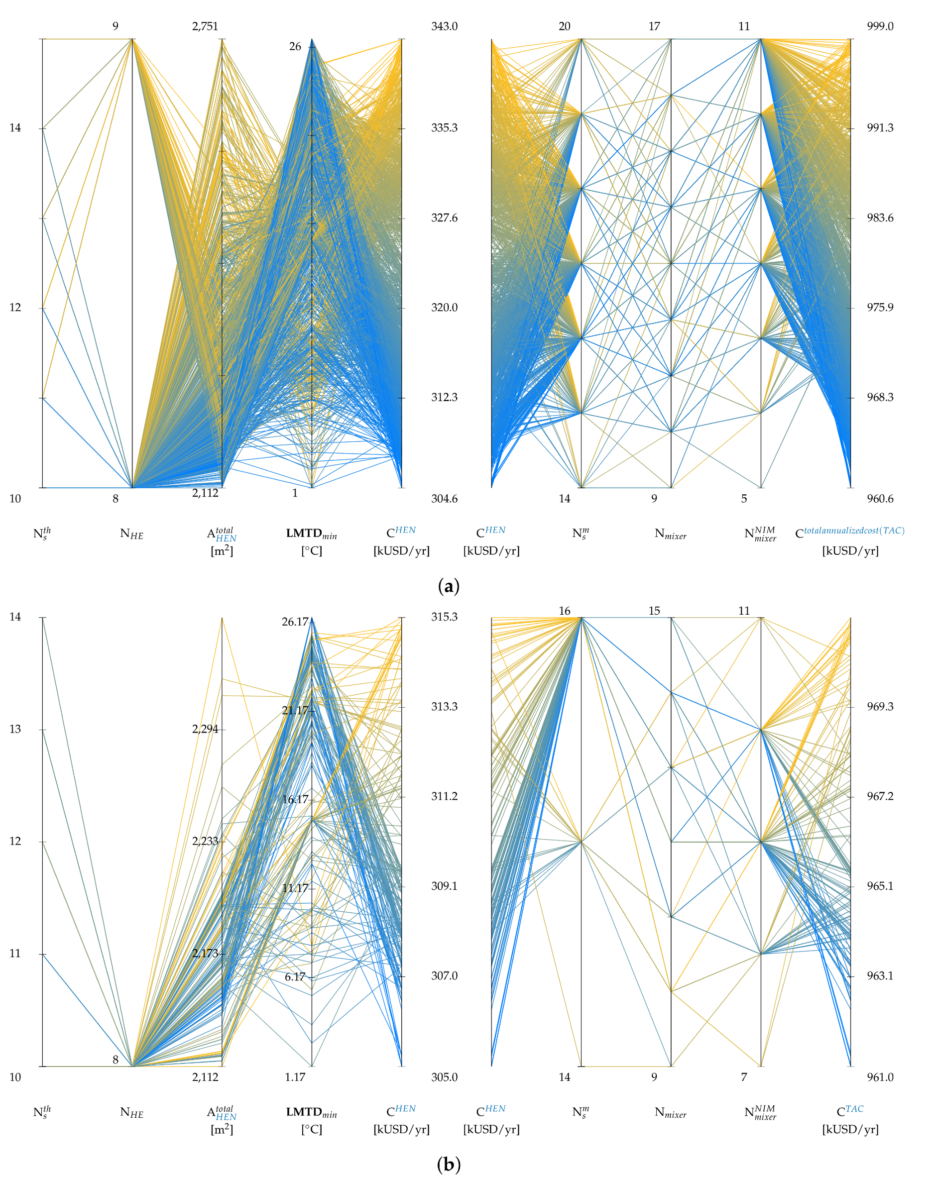
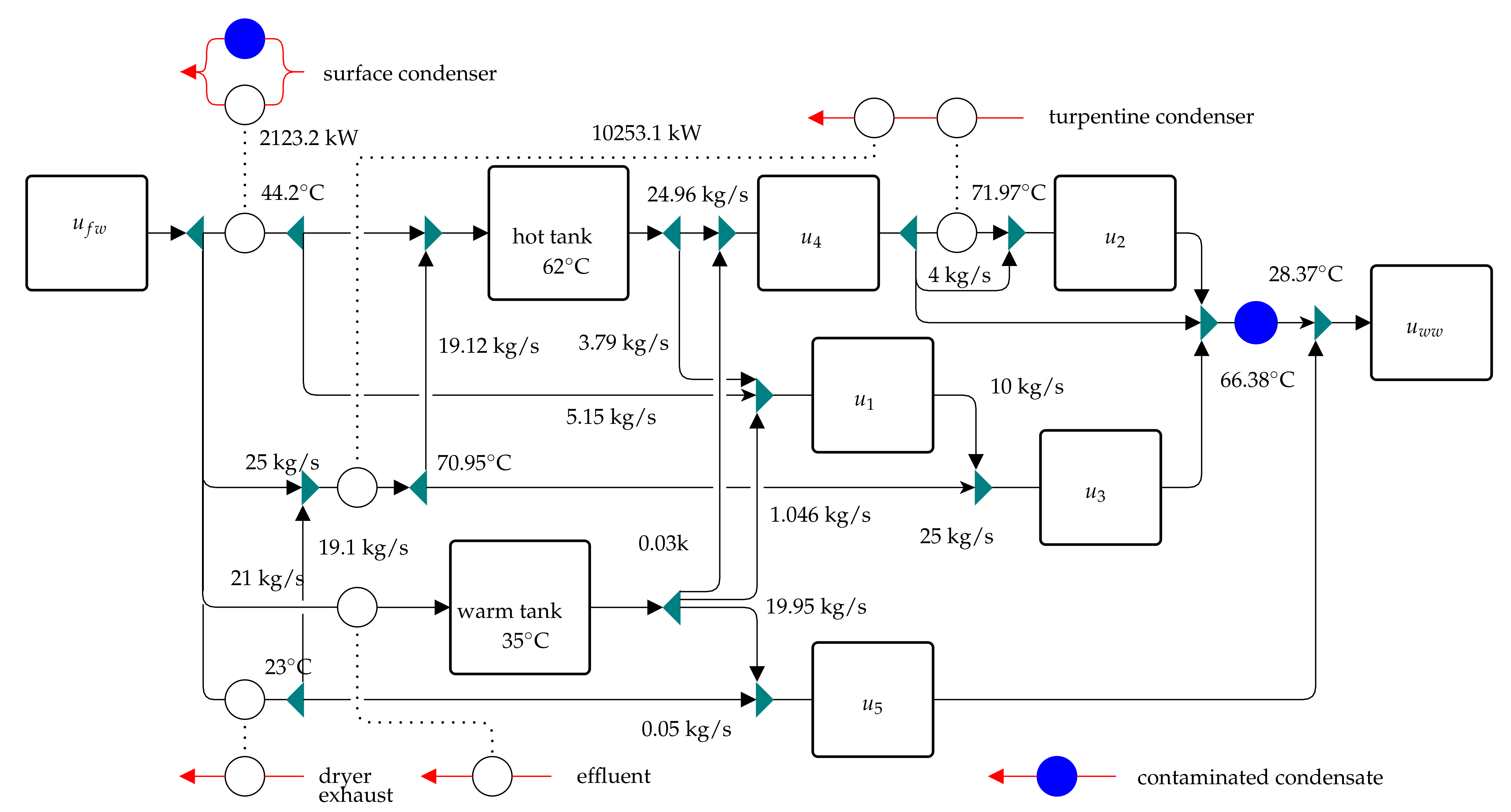
Overall, 2053 solutions satisfy the above criteria which are visualized in Figure 6a (the color spectrum is based on HEN cost). The number of heat exchangers is limited to being 8 or 9, while the area varies between 2100 and 2750 m${}^2$. It can be observed from this figure that, for a given number of mixers and mass streams, the HEN cost varies over the entire range which enunciates that minimizing HEN cost and providing a single solution would not satisfy other important criteria. The lowest total cost reached by the proposed solution strategy is 960.6 kUSD/yr which is less than the lowest reported in the literature (971.4 kUSD/yr [13]). It should also be highlighted that the solution proposed by Ibrić et al. [13] considered the optimization of tank temperatures, while these temperatures are fixed for the analysis presented herein. Moreover, all proposed solutions in this work exhibit 11% lower freshwater consumption than the solutions reported in the literature. Figure 6b illustrates all of the solutions (240) proposed by the sequential solution strategy which exhibit lower total cost than 971.4 kUSD/yr. Figure 6b shows that for a given number of heat exchangers (8 for these solutions), increasing the number of non-isothermal mixing points lowers the total cost. Figure 7 presents one of the optimal HIWAN designs.

Table 4. Comparison of results from the HLD solution (problem P2) and HIWAN hyperstructure (problem P3) based on thermal matches and their heat loads for the optimal solution shown in Figure 7.

Thermal Match	${\mathbf{Q}}_{\mathit{i},\mathit{j}}$ (Problem P2) [kW]	${\mathbf{Q}}_{\mathit{i},\mathit{j}}$ (Problem P3) [kW]
surface condenser → $u_C$	5418.1	5436.8
surface condenser → $u_{fw}^{{70}^{\circ }\mathrm{C}}$	2141.9	2123.2
turpentine condenser → $u_{2,in}^{{62}^{\circ }\mathrm{C}}$	671.9	666.9
turpentine condenser → $u_{fw}^{{70}^{\circ }\mathrm{C}}$	10,248.1	10,253.1
contaminated condensate → $u_C$	630.0	630.0
effluent → $u_{1,out}^{{62}^{\circ }\mathrm{C}}$	105.0	0
effluent → $u_{fw}^{{70}^{\circ }\mathrm{C}}$	2100.0	2205.0
dryer exhaust → $u_{fw}^{{70}^{\circ }\mathrm{C}}$	1050.0	1050.0
$u_{5,in}^{{30}^{\circ }\mathrm{C}}$ → $u_C$	213.9	0
$u_{ww}^{{62}^{\circ }\mathrm{C}}$→$u_C$	9383.1	9578.3

also provides a comparison between problems P2 and P3 in terms of thermal matches and their heat loads for the selected solutions. As described in Section 5, the HLD model and consequently HEN hyperstructure model do not consider stream mixing. The proposed HIWAN model takes these possibilities into account while optimizing the temperatures and flows of heat exchangers. This increases the possibility of replacing a heat exchanger by non-isothermal mixing which led to the elimination of the two smallest heat exchangers as highlighted in Table 4. In both cases, the total heat load of each non-water thermal stream remained constant, while the flow and temperature of water thermal streams adapted to address the shift in the heat load of non-water thermal streams.

7. Conclusions

Two main complexities have been observed within the HIWAN methodologies in the literature. One difficulty is selecting the state of water thermal streams in the HEN design, as this choice affects the overall mathematical formulation in MINLP models. This, in turn, introduces the second difficulty of selecting thermal matches with undefined states of water thermal streams; thus, resulting in a complex MINLP formulation. These two complexities have been addressed by solving problems P1 (targeting model) and P2 (HLD) in sequence prior to the final HIWAN design which identify the states and potential thermal matches, respectively.

A novel HIWAN hyperstructure with NLP formulation has been proposed in this work for the final design of HIWANs which exhibits higher degrees of non-isothermal mixing and lower investment costs. In addition, an iterative sequential solution strategy is proposed in this work by solving the sub-problems with integer cut constraints applied in both problems P1 and P2. As discussed, this approach can be viewed as a technique of reducing the search space at each iteration to a set of potential water thermal streams and a set of potential matches followed by solving the HIWAN synthesis problem for the reduced space.

Applying the proposed methodology on two test cases from the literature illustrated that it is not only able to reach the minimum total system cost (the only objective function used in the literature), but also generates a set of alternative “good” solutions exhibiting various results with respect to other key performance indicators. The first test case, a well-known problem in the literature, yielded 375 solutions with the same (minimum) value of the single objective used. This highlights the plethora of solutions which could be selected by decision-makers to achieve cost targets but with distinguishing features in non-objective or non-quantifiable goals. The second test case yielded 240 alternatives with lower cost than the minimum reported in the literature with an additional benefit of reducing the freshwater consumption by 11%. Similar to the first test case, this reinforces the approach by proposing many “good” solutions which can then be evaluated by engineers or decision-makers based on their other merits. Complexities related to application of the proposed solution strategy and associated MCDM tool on real industrial cases, as the one in a kraft pulp process [15], is limited to characterizing the industrial plant, its specifications, and collecting relevant data.

The proposed approach is intended for the grassroot design of HIWANs and cannot be directly applied to retrofit problems; however, as shown for problem P3, the operating conditions of a water allocation network (i.e., temperatures, flow rates, and heat exchange areas) can be optimized for a given set of thermal matches. Thus, for retrofit cases in which additional heat exchangers are not envisaged, the proposed superstructure can be applied at the current level. For investigating the addition of new heat exchangers, problem P2 can be reformulated by adding new constraints. Multi-period operation of HIWANs (by considering daily/seasonal variations in process operating conditions, temperatures of freshwater, etc.) and uncertainty analysis of HIWANs (to find the most resilient networks given system uncertainties, including costs and operating conditions) should be addressed in future work.

The choice of HEN cost as the main objective in the literature cases should not be the sole measure of optimality, as the basic functions for heat exchanger cost reflect average, observed correlations for overall networks and hence should not be used as the decisive factor in proposing a final design. The proposed approach in this work overcomes this limitation by generating and analyzing a set of solutions and applying multi-criteria optimization to propose competing solutions considering multiple decision criteria.

References

- Jeżowski, J. Review of Water Network Design Methods with Literature Annotations. Ind. Eng. Chem. Res. 2010, 49, 4475–4516. [Google Scholar] [CrossRef]
- Chen, Z.; Wang, J. Heat, mass, and work exchange networks. Front. Chem. Sci. Eng. 2012, 6, 484–502. [Google Scholar] [CrossRef]
- Klemeš, J.J. Industrial water recycle/reuse. Curr. Opin. Chem. Eng. 2012, 1, 238–245. [Google Scholar] [CrossRef]
- Ahmetović, E.; Ibrić, N.; Kravanja, Z.; Grossmann, I.E. Water and energy integration: A comprehensive literature review of non-isothermal water network synthesis. Comput. Chem. Eng. 2015, 82, 144–171. [Google Scholar] [CrossRef]
- Kermani, M.; Kantor, I.D.; Maréchal, F. Synthesis of Heat-Integrated Water Allocation Networks: A Meta-Analysis of Solution Strategies and Network Features. Energies 2018, 11, 1158. [Google Scholar] [CrossRef]
- Karuppiah, R.; Grossmann, I.E. Global optimization for the synthesis of integrated water systems in chemical processes. Comput. Chem. Eng. 2006, 30, 650–673. [Google Scholar] [CrossRef] [Green Version]
- Chew, I.M.L.; Tan, R.; Ng, D.K.S.; Foo, D.C.Y.; Majozi, T.; Gouws, J. Synthesis of Direct and Indirect Interplant Water Network. Ind. Eng. Chem. Res. 2008, 47, 9485–9496. [Google Scholar] [CrossRef]
- Zhou, R.J.; Li, L.J. Simultaneous Optimization of Property-Based Water-Allocation and Heat-Exchange Networks with State-Space Superstructure. Ind. Eng. Chem. Res. 2015. [Google Scholar] [CrossRef]
- Ibrić, N.; Ahmetović, E.; Kravanja, Z.; Maréchal, F.; Kermani, M. Synthesis of single and interplant non-isothermal water networks. J. Environ. Manag. 2017, 203, 1095–1117. [Google Scholar] [CrossRef] [PubMed] [Green Version]
- Kermani, M.; Wallerand, A.S.; Kantor, I.D.; Maréchal, F. A Hybrid Methodology for Combined Interplant Heat, Water, and Power Integration. In Computer Aided Chemical Engineering; Espuña, A., Graells, M., Puigjaner, L., Eds.; Elsevier: Amsterdam, The Netherlands, 2017; Volume 40, pp. 1969–1974. [Google Scholar] [CrossRef]
- Du, J.; Meng, X.; Du, H.; Yu, H.; Fan, X.; Yao, P. Optimal Design of Water Utilization Network with Energy Integration in Process Industries. Chin. J. Chem. Eng. 2004, 12, 247–255. [Google Scholar]
- Kermani, M.; Périn-Levasseur, Z.; Benali, M.; Savulescu, L.; Maréchal, F. An Improved Linear Programming Approach for Simultaneous Optimization of Water and Energy. In Computer Aided Chemical Engineering; Elsevier: Amsterdam, The Netherlands, 2014; Volume 33, pp. 1561–1566. [Google Scholar]
- Ibrić, N.; Ahmetović, E.; Kravanja, Z.; Maréchal, F.; Kermani, M. Simultaneous synthesis of non-isothermal water networks integrated with process streams. Energy 2017. [Google Scholar] [CrossRef]
- Kermani, M.; Périn-Levasseur, Z.; Benali, M.; Savulescu, L.; Maréchal, F. A novel MILP approach for simultaneous optimization of water and energy: Application to a Canadian softwood Kraft pulping mill. Comput. Chem. Eng. 2017, 102, 238–257. [Google Scholar] [CrossRef]
- Kermani, M.; Kantor, I.D.; Wallerand, A.S.; Granacher, J.; Ensinas, A.V.; Maréchal, F. A Holistic Methodology for Optimizing Industrial Resource Efficiency. Energies 2019, 12, 1315. [Google Scholar] [CrossRef]
- Ibrić, N.; Ahmetović, E.; Kravanja, Z. Mathematical programming synthesis of non-isothermal water networks by using a compact/reduced superstructure and an MINLP model. Clean Technol. Environ. Policy 2016, 18, 1779–1813. [Google Scholar] [CrossRef]
- Wang, Y.; Li, R.; Feng, X. Rule-based optimization strategy for energy efficient water networks. Appl. Therm. Eng. 2017, 110, 730–736. [Google Scholar] [CrossRef]
- Ahmetović, E.; Kravanja, Z. Simultaneous synthesis of process water and heat exchanger networks. Energy 2013, 57, 236–250. [Google Scholar] [CrossRef]
- Ahmetović, E.; Kravanja, Z. Simultaneous optimization of heat-integrated water networks involving process-to-process streams for heat integration. Appl. Therm. Eng. 2014, 62, 302–317. [Google Scholar] [CrossRef]
- Papalexandri, K.P.; Pistikopoulos, E.N. A multiperiod MINLP model for the synthesis of flexible heat and mass exchange networks. Comput. Chem. Eng. 1994, 18, 1125–1139. [Google Scholar] [CrossRef]
- Leewongtanawit, B.; Kim, J.K. Synthesis and optimisation of heat-integrated multiple-contaminant water systems. Chem. Eng. Process. Process Intensif. 2008, 47, 670–694. [Google Scholar] [CrossRef]
- Liao, Z.W.; Rong, G.; Wang, J.; Yang, Y. Systematic Optimization of Heat-Integrated Water Allocation Networks. Ind. Eng. Chem. Res. 2011, 50, 6713–6727. [Google Scholar] [CrossRef]
- Hong, X.; Liao, Z.; Sun, J.; Jiang, B.; Wang, J.; Yang, Y. Energy and water management for industrial large-scale water networks: a systematic simultaneous optimization approach. ACS Sustain. Chem. Eng. 2017. [Google Scholar] [CrossRef]
- Yan, F.; Wu, H.; Li, W.; Zhang, J. Simultaneous optimization of heat-integrated water networks by a nonlinear program. Chem. Eng. Sci. 2016, 140, 76–89. [Google Scholar] [CrossRef]
- Sharma, S.; Rangaiah, G.P. Multi-objective Optimization of Heat Integrated Water Networks in Petroleum Refineries. In Computer Aided Chemical Engineering; Elsevier: Amsterdam, The Netherlands, 2014; Volume 33, pp. 1531–1536. [Google Scholar]
- Boix, M.; Pibouleau, L.; Montastruc, L.; Azzaro-Pantel, C.; Domenech, S. Minimizing water and energy consumptions in water and heat exchange networks. Appl. Therm. Eng. 2012, 36, 442–455. [Google Scholar] [CrossRef] [Green Version]
- Hwang, C.L.; Yoon, K. Multiple Attribute Decision Making: Methods and Applications A State-of-the-Art Survey; Lecture Notes in Economics and Mathematical Systems; Springer: Berlin/Heidelberg, Germany, 1981. [Google Scholar]
- García-Cascales, M.S.; Lamata, M.T. On rank reversal and TOPSIS method. Math. Comput. Model. 2012, 56, 123–132. [Google Scholar] [CrossRef]
- Papoulias, S.A.; Grossmann, I.E. A structural optimization approach in process synthesis—II: Heat recovery networks. Comput. Chem. Eng. 1983, 7, 707–721. [Google Scholar] [CrossRef]
- Marechal, F.; Boursier, I.; Kalitventzeff, B. Synep1: A methodology for energy integration and optimal heat exchanger network synthesis. Comput. Chem. Eng. 1989, 13, 603–610. [Google Scholar] [CrossRef]
- Floudas, C.A.; Ciric, A.R. Strategies for overcoming uncertainties in heat exchanger network synthesis. Comput. Chem. Eng. 1989, 13, 1133–1152. [Google Scholar] [CrossRef]
- Inselberg, A. The plane with parallel coordinates. Vis. Comput. 1985, 1, 69–91. [Google Scholar] [CrossRef]
- Cajot, S.; Mirakyan, A.; Koch, A.; Maréchal, F. Multicriteria Decisions in Urban Energy System Planning: A Review. Front. Energy Res. 2017, 5. [Google Scholar] [CrossRef] [Green Version]
- Cajot, S.; Schüler, N.; Peter, M.; Koch, A.; Maréchal, F. Interactive Optimization With Parallel Coordinates: Exploring Multidimensional Spaces for Decision Support. Front. ICT 2019, 5. [Google Scholar] [CrossRef] [Green Version]
- Chen, J.J.J. Comments on improvements on a replacement for the logarithmic mean. Chem. Eng. Sci. 1987, 42, 2488–2489. [Google Scholar] [CrossRef]
- Savulescu, L.E.; Smith, R. Simultaneous energy and water minimisation. In Proceedings of the 1998 AIChE Annual Meeting, Miami Beach, FL, USA, 15–20 November 1998; pp. 13–22. [Google Scholar]
- IBM ILOG CPLEX V12.2: User’s manual for CPLEX; Technical report; IBM Corporation: Armonk, NY, USA, 2010.
- Gill, P.E.; Murray, W.; Saunders, M.A. User’s Guide for SNOPT Version 7: Software for Large-Scale Nonlinear Programming; Technical report; Center for Computational Mathematics; University of California: San Diego, CA, USA, 2008. [Google Scholar]
- Fourer, R.; Gay, D.M.; Kernighan, B.W. AMPL: A Modeling Language for Mathematical Programming, 2nd ed.; Cengage Learning: Boston, MA, USA, 2003. [Google Scholar]
- Savulescu, L.; Kim, J.K.; Smith, R. Studies on simultaneous energy and water minimisation—Part I: Systems with no water re-use. Chem. Eng. Sci. 2005, 60, 3279–3290. [Google Scholar] [CrossRef]
- Savulescu, L.; Kim, J.K.; Smith, R. Studies on simultaneous energy and water minimisation—Part II: Systems with maximum re-use of water. Chem. Eng. Sci. 2005, 60, 3291–3308. [Google Scholar] [CrossRef]
- Wan Alwi, S.R.; Ismail, A.; Manan, Z.A.; Handani, Z.B. A new graphical approach for simultaneous mass and energy minimisation. Appl. Therm. Eng. 2011, 31, 1021–1030. [Google Scholar] [CrossRef]
- Maréchal, F.; Kalitventzeff, B. Process integration: Selection of the optimal utility system. Comput. Chem. Eng. 1998, 22 (Suppl. 1), S149–S156. [Google Scholar] [CrossRef]
- Kermani, M.; Wallerand, A.S.; Kantor, I.D.; Maréchal, F. Generic superstructure synthesis of organic Rankine cycles for waste heat recovery in industrial processes. Appl. Energy 2018, 212, 1203–1225. [Google Scholar] [CrossRef]
Figure 1.
Schematic of the proposed source and sink hyperstructures based on HEN hyperstructure [31] (dashed arrows indicate flows among hyperstructures of the same source or the same sink similar to the definition of and ). (a) HEN hyperstructure; (b) Source hyperstructure for HIWAN; (c) Sink hyperstructure for HIWAN.
Figure 2.
Iterative sequential solution strategy proposed for solving HIWAN synthesis problems.
Figure 3.
Illustrative case: (a) results of problem P1 and P2, (b) construction of the HIWAN hyperstructure.
Figure 4.
Comparison of two approaches for HEN design in water networks (dashed lines are unselected options of the related hyperstructure). (a) HEN design using NLP-hyperstructure of Floudas and Ciric [31]; (b) HEN design using NLP-hyperstructure of HIWAN proposed in this work.
Figure 5.
Visualization of key indicators of test case I using parallel coordinates for (a) all solutions and (b) solutions with lowest HEN cost. (The color spectrum is based on HEN cost which varies from blue (the lowest) to yellow (the highest)). (a) All 2247 solutions (test case I); (b) Solutions with the lowest HEN cost (test case I).
Figure 6.
Visualization of key indicators of the simplified kraft case using parallel coordinates for (a) all solutions and (b) solutions with lowest HEN cost (The color spectrum is based on HEN cost which varies from blue (the lowest) to yellow (the highest)). (a) All 2053 solutions; (b) Solutions with lower TAC cost than the value reported in the literature (240 solutions).
Figure 7.
One of the optimal solutions for the simplified kraft test case exhibiting improved performance: = 80 kg/s, = 15,645 kW, N = 8, A = 2147.9 m, = 26.46 C, C = 306.78 kUSD/yr, C = 656.0 kUSD/yr, C = 962.8 kUSD/yr, N = 16, N = 11, N = 9.