Automatic Coordination of Internet-Connected Thermostats for Power Balancing and Frequency Control in Smart Microgrids

Abstract

This paper proposes a novel feedback control strategy, so-called clock-like controller (CLC), to balance power supply and demand in smart microgrids by adjusting the setpoint temperatures of air conditioning (AC) loads. In the CLC algorithm, the grid operator communicates with the individual thermostats via the Internet and adjusts their setpoints by discrete temperature intervals (e.g., ±0.5 °C). Numerical simulations indicate that the proposed algorithm is able to deliver a smooth controllability of the aggregate AC power despite discrete temperature offsets. It can also be used for peak load shedding to mitigate the power generation cost. The CLC algorithm is then integrated into the grid frequency control problem, in which both power generators and loads in the network attempt to regulate the frequency of the system despite disturbances from demand, renewable sources, and local weather conditions. An autonomous microgrid model including a steam and a hydro generator, a solar energy source, and a large number of thermostatic loads is developed to evaluate and demonstrate the proposed method. Simulation results indicate that the AC loads with CLC algorithm can help maintain the power system frequency during extreme events when demand exceeds the maximum generation capacity available to the network. Under normal conditions, the contribution of demand-side control is marginalized by the fast responding generators, because of time delays in the frequency measurement and internet communication network.

1. Introduction

This paper addresses the problem of power balancing and frequency control in smart autonomous microgrids using the setpoint adjustment of internet-connected thermostats. Due to the large thermal capacity of residential buildings, and relative flexibility in their temperature setpoints, heating and cooling loads offer a great potential for energy management in smart grids. This paper contributes to the literature in at least three different ways. First, unlike most previous methods which adjust the setpoint temperatures of the loads concurrently and continuously, the proposed control scheme offsets the setpoints in discrete intervals, e.g., ±0.5 °C, to facilitate implementation through the currently available infrastructure, i.e., the Internet. Secondly, the proposed algorithm provides a systematic mechanism to call the loads without any random selection process, to enable fair and equal contribution of all participating loads. Last, this paper develops a grid frequency control system for thermostatic loads in the presence of active automatic generation control, and investigates scenarios in which demand-side frequency control can be effective.

Demand-side energy management has been the subject of many research studies in the past few decades. Since the emergence of smart grid, electric vehicles and thermostatically-controlled thermal loads have been at the center of attention for demand-side energy management [1,2]. Various types of thermostatic loads have been investigated in the literature, including air conditioning systems [3,4], water heaters [5,6], and refrigerators [7]. In most of these studies, setpoint temperature has been selected as the primary control variable, through which the grid operator can access the loads and alter their thermal response based on the grid needs. Renewable energy balancing by power tracking [3,4], frequency regulation [7,8,9], and peak load shedding [10,11] are the most commonly-adopted control objectives. Direct on-off scheduling using a predicted electricity price signal [12,13], energy management based on packet scheduling algorithms [14,15], and privacy preserving-based management strategies [16] have also been studied in the recent literature.

Aggregate power of thermostatic loads has been generally modeled in at least four different ways. The first approach is to simulate a large number of individual load dynamics with randomized parameters and initial conditions, and then aggregate them to replicate a realistic system [3,4,17]. This method, also known as the Monte Carlo approach, is the closest approximation to practice for validating the performance of demand-side controllers. For controller design, however, some studies have looked into developing control-oriented partial differential equation models for the distribution of loads on the thermostatic on and off states. These models are either represented in the form of diffusion [3,17,18] or transport PDE [4], and can be used directly or in the discrete form for stability analysis. The third modeling approach is to approximate the aggregated power dynamics using a linear second order transfer function. These models are developed for both setpoint temperature offset [19] and ambient temperature [20] as the external system inputs. Finally, state queuing [21,22] or stochastic Markov chain [23] models have been developed, which discretize the thermostatic temperature range in a finite number of states and capture load distribution dynamics using matrix-based state transition formula. These models are primarily developed for heterogeneous loads, and tend to provide good approximation of the Monte Carlo model.

Grid frequency control is one of the main operations targeted by demand-side energy management studies. Traditionally, power generators on the grid are responsible for correcting frequency deviations through a process called frequency droop control [24]. In multi-area power networks, automatic generation control (AGC) is used to simultaneously regulate frequency and tie-line power flows between neighboring areas through area control error (ACE) signal [24]. Under AGC, a selected number of generators are equipped with integral controllers, which gradually lift the burden from the initially responding generators, thereby allowing them to return to their scheduled setpoints. The frequency droop controllers stabilize frequency within 3–5 s upon an event. For the demand-side frequency controllers to be effective, a similar or faster response time is required. Given the time delays present in the communication infrastructure and internal load dynamics, competing with the generation-side controllers seems to be a very challenging task.

For microgrids with energy storage recourses such as electric vehicles, different frequency control methods have been proposed, such as model-free sliding mode control [25] and fuzzy logic-based optimal PID controllers [26,27]. Moreover, other load types such as household air conditioning systems and refrigerators have been adopted for grid frequency stabilization [7,9]. These methods are primarily developed around the assumption that the setpoint temperatures of the responding loads can be varied continuously and simultaneously using a centrally broadcast signal or an onboard measurement device for grid frequency. Presently, the market is being dominated by smart internet-connected thermostats under different brand names such as Honeywell, Nest or Ecobee. These thermostats are connected to a central server and can be managed by the user via the thermostat’s controls or a computer application. Moreover, the users may opt in to a demand-response program and allow the central server to temporarily control the system in exchange for an economic incentive.

The setpoint temperatures in the smart thermostats can only be shifted by discrete intervals (e.g., ±0.5 °C or ±1 °F) due to sensor limitations and simplicity of operation. Therefore, many control logics that have been developed based on continuous temperature offset strategy cannot be employed in the current infrastructure. This paper attempts to address this problem by proposing a systematic control framework for internet-connected smart thermostats, building significantly on an earlier publication [28]. The control logic is reformulated for a variety of control problems such as power tracking, peak load shedding, and frequency regulation in the presence of AGC. Several microgrid-level simulations are presented to demonstrate the strengths and deficiencies of the proposed method in different real-word scenarios.

The remainder of the paper is organized as follows: Section 2 presents the model used for simulating the aggregate power of a large number of air conditioning loads. Section 3 formulates the proposed controllers for power tracking and peak-load shedding, along with a mechanism for protecting user comfort. Section 4 formulates the frequency regulation problem in the presence of an automatic generation control system. Numerical simulations are included in all the three sections to evaluate and validate the proposed models and algorithms. Finally, Section 5 summarizes the paper’s key conclusions.

2. Aggregate AC Load Model

In this section, an aggregate AC load model is developed by modeling each AC system with a first-order thermal differential equation as follows [3]:

$${\dot{T}}_i=\frac{1}{C_i{R}_i}\left(T_{\infty }-T_i-s_i\left(t\right)R_i{Q}_i\right),i=1,2,\dots ,N_{AC}$$

(1)

where i is the load index, $T$ and $T_{\infty }$ represent the indoor and ambient temperatures, respectively, C and R are the thermal capacity and thermal resistance of the building, Q is the energy transfer rate by the AC system, and s is the thermostatic switching controller described as:

$$s_i\left(t\right)=\{\begin{array}{cc}0,& if{s}_i\left(t-\epsilon \right)=1and{T}_i\left(t\right)\le T_{min,i}\\ 1,& if{s}_i\left(t-\epsilon \right)=0and{T}_i\left(t\right)\ge T_{max,i}\\ s_i\left(t-\epsilon \right),& otherwise\end{array}$$

(2)

where ε is an infinitesimal time delay to facilitate the formulation of the thermostatic switching (relay) function in continuous time. $T_{min}$ and $T_{max}$ represent the lower and upper temperature bounds of the thermostat, respectively. These quantities are related to the setpoint temperature ($T_{sp}$) and the thermostat’s dead-band ${\delta }_{db}$.

$$T_{min,i}=T_{sp,i}-\frac{{\delta }_{db}}{2},T_{max,i}=T_{sp,i}+\frac{{\delta }_{db}}{2}$$

(3)

The aggregate AC power is the summation of individual AC powers adjusted by their respective coefficient of performance (η):

$$P_{Agg}\left(t\right)={\displaystyle \sum }_{i=1}^{N_{AC}}{s}_i\frac{Q_i}{{\eta }_i}$$

(4)

In this study, we assume that the grid operator is able to communicate with the individual thermostats and offset the setpoint temperatures up or down by a limited amount applied separately to each thermostat:

$$T_{sp,i}\left(t\right)=T_{sp0,i}+u_i\left(t\right)T_{step,i}$$

(5)

where $T_{sp,0}$ represents the user-specified setpoint value, $T_{step}$ is the temperature step (e.g., 0.5 °C, 1 °C, or larger), and u is a signed integer determining the number of temperature steps away from the user setpoint.

Simulink provides a simple way to simulate the system in the block diagram form as shown in Figure 1. All the parameters and signals have been vectorized to simplify the Simulink model. The AC temperatures are initialized inside the integrator, and a custom relay function is developed based on Equation (2) to allow arbitrary initial values for the switching state, s. The 1st order Euler ODE solver is used to enable simulation of discrete-time clock-like controller discussed in the next section. The parameters of the system are adopted from [3] and given in

Table 1. System parameters adopted from [3].

Parameter	Mean Value	Unit	Rel. Stand. Deviation
R, Thermal Resistance	2	°C/kW	0.1
C, Thermal Capacitance	10	kWh/°C	0.1
η, Coefficient of Performance	$2.5$	-	0.0
δdb, Thermostat Deadband	0.5	°C	0.0
Q, Energy Transfer Rate	14	kW	0.1

. The table also contains a column on the relative standard deviation of the parameters used to create a realistic population from normal parameter distributions.

To simulate the aggregate system response, a 24-h ambient temperature profile is created based on temperature data for the city of San Jose, California, in a warm summer day. The number of loads (N_AC) is set to be 5000 to create a smooth aggregate response. The setpoint temperatures are distributed normally with 21.0 °C (~70 °F) mean value and 10% relative standard deviation. These values are then rounded to the nearest half degree value to create a discrete distribution with 0.5 °C intervals. The system is simulated first with temperatures initially set to be the same as the initial ambient temperature. The simulation is then repeated by setting the initial temperature values same as the final temperature values from the first run. This would represent a more realistic simulation, as the initial temperatures are dependent on the historical ambient temperature trajectory and the user setpoints.

Figure 2 shows the simulation result, with the ambient temperature, aggregate AC power, and five sample indoor temperature trajectories with five different setpoint values plotted. As can be seen, the aggregate power (divided by the number of loads) increases as the ambient temperature rises. However, there is a time delay of around 1–2 h between the ambient temperature peak and the aggregate AC power peak due to the thermal capacitance of the loads. During peak time, the aggregate AC power reaches to around 30% of the maximum power the ACs can possibly demand (1.6 kW vs. 5.6 kW max power per AC unit). This is because of the fact that the loads turn on and off at different times due to different initial conditions and thermal properties. For this simulation, an outdoor-indoor temperature difference of around 28 °C can push the AC to remain always on, according to Equation (1) when $\dot{T}$ = 0, and using the nominal values in Table 1.

The simulation in this section shows that the setpoint temperature impacts the AC demand. From the sample temperature trajectories in Figure 2, we can see that the total power-on duration is longer for loads with lower setpoint temperatures. This behavior motivates us to develop an algorithm that provides controllability over the aggregate AC demand through adjustment of the setpoint temperatures via internet-connected smart thermostats.

3. Aggregate Power Control using Clock-Like-Controller

Since temperature intervals are discrete in smart thermostats, the aggregate power controller cannot send temperature step commands to all AC units simultaneously. Otherwise, large power fluctuations will occur with all AC units turning off or on simultaneously. Therefore, the setpoints must be adjusted selectively at different times based on the system needs. In this study, a clock-like control (CLC) framework is introduced for the systematic management of aggregate AC power. The goal of the CLC method is to (i) provide a smooth control over the aggregate AC power, and (ii) avoid randomized selection schemes, and engage all the participating loads in a fair and equal way.

The CLC system includes a clock face (dial) whose periphery is numbered from 1 through the total number of AC units, N_AC (see Figure 3). The clock has two hands that can rotate in the clock-wise direction only, and meet all of the AC units in one full turn. When one of the clock hands crosses an AC unit sector, it increases its setpoint temperature by one temperature step (e.g., 0.5 °C). The other clock hands steps down the setpoint temperature of the AC unit it crosses. We can therefore modify the aggregate AC power response by increasing and decreasing the setpoint temperatures of the individual ACs through the rotation of the two clock hands. A feedback control algorithm can provide the required angular positions of the clock hands to deliver the ultimate aggregate power tracking objective.

3.1. Feedback Control Formulation Using the CLC Method

The objective of the CLC scheme is to balance the power supply and demand within the microgrid when AC units are active. We assume that the controller is only provided with the tracking error, defined as:

$$e\left(k\right)=\{\begin{array}{c}{P}_{Sup}\left(k\right)-P_{Dem}\left(k\right),Heating\\ P_{Dem}\left(k\right)-P_{Sup}\left(k\right),Cooling\end{array}$$

(6)

The determination of heating or cooling mode is based on the majority of the loads. It is reasonable to assume that the demand-side control is only effective during sufficiently warm or cold days, when the AC units are actively heating or cooling. When there is a mix of heating and cooling loads in moderately warm or cool days, the aggregate power will be insignificant, and therefore not useful for demand-side control.

To develop a control law for the two clock hands, we first define the positive and negative error signal as:

$$e_p\left(t\right)=\{\begin{array}{c}e\left(t\right),ife\left(t\right)>0\\ 0,ife\left(t\right)\le 0\end{array}$$

(7)

$$e_n\left(t\right)=\{\begin{array}{c}e\left(t\right),ife\left(t\right)<0\\ 0,ife\left(t\right)\ge 0\end{array}$$

(8)

An integral controller is then used to rotate the clock hands based on the positive or negative error:

$${\theta }_p\left(t\right)=K_{i,p}{{\displaystyle \int }}_0^t{e}_p\left(\tau \right)d\tau$$

(9)

$${\theta }_n\left(t\right)=-K_{i,n}{{\displaystyle \int }}_0^t{e}_n\left(\tau \right)d\tau$$

(10)

where K_i,p and K_i,n are the integral gains, determining the rotation rate of the clock hands based on the power error. These gains must be positive for the cooling, and negative for the heating loads, for the CLC to function correctly.

To link the clock hand positions to the AC units on the clock periphery, a certain time interval must be dedicated to observe the rotation of the clock hands. Therefore, the CLC scheme has to be implemented in the discrete-time form.

At a given time, t, the index of the AC unit pointed by the positive or the negative clock hand can be calculated from:

$$z_p\left(t\right)=\lceil \left(\frac{{\theta }_p\left(t\right)}{2\pi }-\lfloor \frac{{\theta }_p\left(t\right)}{2\pi }\rfloor \right)N_{AC}\rceil$$

(11)

$$z_n\left(t\right)=\lceil \left(\frac{{\theta }_n\left(t\right)}{2\pi }-\lfloor \frac{{\theta }_n\left(t\right)}{2\pi }\rfloor \right)N_{AC}\rceil$$

(12)

where $\lfloor ·\rfloor$ and $\lceil ·\rceil$ indicate the floor and ceiling operations, respectively.

The setpoint temperature change for AC unit $i,\left(i\in \left\{1,\dots ,N_{AC}\right\}\right)$ can be calculated from:

$$\begin{gathered} \Delta u_i\left(k\right)\{\begin{array}{cc}1& if{z}_p(k-1)<i\le z_p\left(k\right)or \\ i\le z_p\left(k\right)<z_p(k-1)or \\ {z}_p\left(k\right)<z_p(k-1)<i\\ -1& if{z}_n(k-1)<i\le z_n\left(k\right)or \\ i\le z_n\left(k\right)<z_n(k-1)or \\ {z}_n\left(k\right)<z_n(k-1)<i\\ 0& otherwise\end{array} \end{gathered}$$

(13)

where $\Delta u_i\left(k\right)=u_i\left(k\right)-u_i\left(k-1\right)$, with k being the discrete time index (k = t/Δt). Note that f(k) is the simplified version of f(kΔt), representing the discrete-time function at time t or time step k.

Equation (13) summarizes the formulation of the CLC algorithm. When the AC unit index is swept by one of the clock hands within a certain time interval Δt, the setpoint temperature for that load is changed by one temperature step up or down. The reason we have three conditions for the setpoint offsets is due to the fact that we wrap θ between 0 to 2π in the computation of AC index, z. Although z is a normally increasing signal, i.e., $z\left(k\right)\ge z\left(k-1\right)$, there are times when the value of z(k) is reset because of the clock hand crossing 2π, thereby dropping below $z\left(k-1\right)$. In such events, one portion of the covered load sectors lie between $z\left(k-1\right)$ to N_AC, and another part between 1 to z(k), adding two more conditions per clock hand to the setpoint offset event.

3.2. Accounting for End-User Comfort

To ensure positive end-user response, a certain limit must be applied to the setpoint temperature offset signals to maintain the indoor temperature near the user specified value. This limit can be imposed in the CLC scheme by limiting the difference between clock hand positions. If the clock hands are separated by 2π at a given time, all the homes have experienced one full temperature step deviation from the initial setpoint. Therefore, a limit of 2π seems to be a reasonable limit. To impose a 2π limit on the separation of the clock hands, the integral control laws can be modified to:

$${\theta }_p\left(t\right)=K_{i,p}{{\displaystyle \int }}_0^t{\mathrm{Proj}}_{\Delta \theta }\left[e_p\left(\tau \right)\right]d\tau$$

(14)

$${\theta }_n\left(t\right)=-K_{i,n}{{\displaystyle \int }}_0^t{\mathrm{Proj}}_{\Delta \theta }\left[e_n\left(\tau \right)\right]d\tau$$

(15)

where:

$$\Delta \theta \left(t\right)={\theta }_p\left(t\right)-{\theta }_n\left(t\right)$$

(16)

$${\mathrm{Proj}}_{\Delta \theta }\left[e_p\left(t\right)\right]=\{\begin{array}{ll}0& if\Delta \theta \left(t\right)\ge 2\pi and{e}_p\left(t\right)>0\\ e_p\left(t\right)& otherwise\end{array}$$

(17)

$${\mathrm{Proj}}_{\Delta \theta }\left[e_n\left(t\right)\right]=\{\begin{array}{ll}0& if\Delta \theta \left(t\right)\le -2\pi and{e}_n\left(t\right)<0\\ e_n\left(t\right)& otherwise\end{array}$$

(18)

The role of the projection operation is to simultaneously clamp the separation of the clock hands, and prevent the integrator windup by setting the integrant to zero during the clamp period.

3.3. CLC Simulations

To demonstrate the CLC system response, a Simulink diagram is created first as shown in Figure 4. The upper diagram demonstrates the single-input, single-output feedback loop for the system, and the lower diagram shows the single-input, multi-output CLC subsystem, where the power supply and demand error is received as the input and the control vector u is calculated as the output. Two MATLAB functions are used to program the projected positive and negative errors before integration, i.e., Equations (17) and (18), and the CLC indexing and activation logic, i.e., Equations (11)–(13). Similar to the aggregate AC model, the CLC is implemented in the vector form at and after the second MATLAB function’s output. Once the control vector u is computed, it gets broadcast to all participating thermostats via internet. Each thermostat receives one element of u and responds accordingly. In practice, a time delay in the order of a few seconds may be involved in the internet communication, which is accounted for in the Simulink model.

The first simulation is to track a desired power trajectory comprising both smoothly varying and abruptly changing components as shown in Figure 5. The purpose of this simulation is to evaluate how CLC can respond to different conditions on the grid, such as smooth ramping or sudden changes due to contingencies. The ambient temperature is set to be 30 °C, and kept constant throughout the simulation. The setpoint temperature step is set to be 0.5 °C for all loads, and the communication delay is set to 5 s. To make sure the room temperatures remain near the user setpoint, the average value of desired power is matched with that of the natural aggregate power of the ACs. Mismatch in the desired vs. natural power for a long period of time may result in a continuous drift in one of the clock hands, thereby leading to control saturation.

As can be seen in Figure 5a, the aggregate AC power is able to closely track the desired power trajectory in the smooth (sinusoidal) segment. During abrupt changes, the aggregate power is able reach and stay around the desired level within about 1 min. There is a time period between hours 11:00–12:00 where the aggregate power parts way from the desired power. This is due to the implemented control saturation function, which limits clock hand separation within ±2π to enforce user comfort. As can be seen from Figure 5b, the clock hand separation angle hits the lower limit between hours 11:00–12:00 to prevent setpoint temperature migration beyond the intended ±0.5 °C level. The clock hand separation, however, remains within ±2π for most part, providing control over the aggregate power. Figure 5c shows a sample indoor temperature trajectory under the provided simulation, compared to the natural (uncontrolled) response. In this example, the natural temperature varies between 19.75 °C to 20.25 °C, whereas the controlled temperature varies between 19.25 °C to 20.75 °C, which are ±0.5 °C apart from the limits of the natural response.

To provide a more realistic simulation, the application of the proposed control method in peak load shaving scenario is studied next. We apply the ambient temperature trajectory in Figure 2, resulting in the peak aggregate power of 1.65 kW per AC unit, around 3 pm. The control objective in this simulation is to limit the peak power at or below a particular level, e.g., 1 kW per AC unit, using the CLC method. To enable this process, a modification is needed in the CLC algorithm. We only need to activate the CLC controller when the aggregate power demand goes beyond the desired level, and that happens when the tracking error is positive (in the case of cooling loads). Therefore, we can simply let e_n = 0 in the controller to allow natural AC operation below the desired power limit. A second modification is to bring the setpoint temperatures back to their initial values by driving the clock hand angle difference to zero once the event is cleared. A simple and creative way to enable this effect is to modify the negative error definition as follows:

$$e_n\left(t\right)=\{\begin{array}{ll}-\alpha \Delta \theta \left(t\right),& ife\left(t\right)<0\\ 0,& ife\left(t\right)\ge 0\end{array}\left(PeakShaving\&Cooling\right)$$

(19)

where α is a scaling factor, determining the convergence rate of clock hands toward each other. Based on this revised formula, the CLC will correct the separation angle when the power demand falls below the limit. To further analyze the controller dynamics when e(t) < 0, we can replace the revised e_n in the integral control law (Equation (10)), and take time derivative to get:

$${\dot{\theta }}_n\left(t\right)+\alpha K_{i,n}{\theta }_n\left(t\right)=\alpha K_{i,n}{\theta }_p\left(t\right)$$

(20)

which indicates ${\theta }_n\to {\theta }_p$ as $t\to \infty$ if $\alpha K_{i,n}>0$.

Figure 6 shows the peak load shaving simulations. The aggregate AC power for the cases of natural (uncontrolled) scenario, and controlled scenario, with and without setpoint correction, are shown in Figure 6a. The peak shaving objective is fairly achieved in both controlled cases. However, when the setpoint correction mechanism is implemented (based on Equation (19)), there is a payback period after the natural response falls below the limit. This is due to the fact that, setpoint correction requires the ACs to cool down to the initial temperature setpoints. Figure 6b compares the clock hands separation angle for the two cases, indicating an exponential converge of the angle separation to zero, as anticipated from Equation (20). The convergence of angle separation to zero is necessary for two reasons: (i) returning the occupants’ comfort, and (ii) preparing for the next day operation by bringing the control signal back to the middle position. To show the impact of the control process, a sample load temperature trajectory is shown in Figure 6c. Under the peak load shaving controller, the indoor temperature rises by half a degree above the normal thermostatic range, but is then returned to the range through the setpoint correction mechanism.

4. Microgrid Frequency Control using AGC and CLC

Frequency stability is becoming an increasingly important problem in microgrids due to the growth of disturbances introduced by uncontrollable renewable resources. Traditionally, load frequency control (LFC) and automatic generation control (AGC) methods are used to stabilize grid frequency [24]. With automatic demand-side control, additional stability margin can be introduced to the system. Understanding the dynamic interactions between generation-side and demand-side control has not been investigated in the literature in a good depth. This section attempts to provide some insights into how thermostatic loads can cooperate with AGC to improve grid frequency stability.

4.1. Automatic Generation Control Model

A well-stablished model for AGC is used in this paper to evaluate the simultaneous demand-side and generation-side frequency control problem. This model is based on the frequency droop control in power plants serving the grid in conjunction with integral controllers on selected power plants [24]. Assuming the grid voltage and the frequency dynamics are decoupled, the frequency control problem is reduced to an equivalent single-inertia system, relinquishing the need for network topology. In this paper, a hybrid generation system comprising a steam and a hydro power plant is used for the generation-side microgrid control based on models in [24], as shown in Figure 7. The steam plant has a second order dynamics, and the hydro plant has a non-minimum-phase first order transfer function. These models are the linearized versions of complex physics-based nonlinear models [24], and are suitable for stability analysis and control design. Both power plants are equipped with speed governors (controllers), which respond to changes in frequency immediately after an event (sudden change in load), by adjusting the fuel valve or water valve positions. Besides, the steam power plant is equipped with an integral controller which is responsible for bringing the frequency back to the target level (e.g., 60 Hz) after the initial response from the droop controllers. This way, the steam generator becomes the main power plant in charge of tracking slow changes in the load, and the hydro power plant provides additional bandwidth to suppress the transient disturbances.

The output from the power plants is subtracted from the load, resulting in a net power imbalance in the system. A first order linearized model is traditionally used for analyzing the grid’s inertial dynamics, and is adopted in this study as shown in Figure 7. This model includes two parameters, accounting for the collective grid rotor inertia through time constant M, and the load damping factor, through constant D. The entire generation-side system is represented in the normalized per-unit (pu) system for the simplicity of analysis and consistency with the literature. The parameters of the system used for the simulations of this section are adopted from [24] and listed in

Table 2. Generation-side system parameters adopted from [24].

Parameter	Value	Parameter	Value
M	10.0 s	D	1.0
Rs	0.05	Rh	0.05
TG	0.2 s	TG,h	0.2 s
FHP	0.3	RT	0.38
TRH	7.0 s	TR	5.0 s
TCH	0.3 s	TW	1.0 s

. Most of the parameters are various time constants associated with the response time of the power plants and the controllers. As can be seen, all the time constants are within 10 s, which indicates the frequency can be recovered within a few seconds after an event. In practice, there are limits on the ramping rate of the power plants, which would impact frequency recovery depending on the size of the disturbance. An improved generation-side model is used in the next section to account for these limits.

To simulate the AGC system response, a 5% step increase in load is applied to the system at t = 10 s, and response of the system is recorded for 2 min. Figure 8 shows the frequency deviation in pu, as well as the power plants responses to the step disturbance with and without integral controller on the steam plant.

As can be seen in both cases, the frequency is recovered within a few seconds. The system with integral controller is able to eliminate the steady-state error within a few minutes (with K_i,AGC value of 1). Without the integral controller, both power plants share 50% of the load at steady state due to identical frequency droop coefficients (R_h = R_s). With integral controller, however, the steam plant takes the full burden of the load at steady-state, allowing the hydro plant to go back to its initial state after the preliminary reaction.

4.2. Clock-Like Frequency Controller (CLFC) for Thermostatic Loads

To control grid frequency through internet-connect thermostatic loads, the control error signal is changed from power imbalance in CLC to frequency deviation in CLFC. Therefore, the control strategy must be changed accordingly. Due to the first order dynamic relation between the frequency and power imbalance, a modified error signal is created and used as input to the controller, combining frequency deviation and its time derivative as follows:

$$\xi \left(t\right)=\{\begin{array}{cc}\sigma \dot{\Delta f}\left(t\right)+\Delta f\left(t\right),& Heating\\ -\sigma \dot{\Delta f}\left(t\right)-\Delta f\left(t\right),& Cooling\end{array}$$

(21)

where σ is a positive control parameter, determining the weight of the time derivative of the frequency error in the control process. This modification builds a predictive response in the controller to take action before the frequency deviates significantly. It is also consistent with other methods proposed in the literature for grid frequency control using thermostatic loads [9].

The positive and negative error signals for frequency control are then defined as:

$${\xi }_p\left(t\right)=\{\begin{array}{ll}\xi \left(t\right)& if\xi \left(t\right)>{\epsilon }_f\\ -\alpha \Delta \theta \left(t\right)& if\left|\xi \left(t\right)\right|\le {\epsilon }_{f}and\Delta \theta \left(t\right)<0\\ 0,& otherwise\end{array}$$

(22)

$${\xi }_n\left(t\right)=\{\begin{array}{ll}\xi \left(t\right)& if\xi \left(t\right)>{\epsilon }_f\\ -\alpha \Delta \theta \left(t\right)& if\left|\xi \left(t\right)\right|\le {\epsilon }_{f}and\Delta \theta \left(t\right)<0\\ 0,& otherwise\end{array}$$

(23)

where $-\alpha \Delta \theta \left(t\right)$ is the correction term to bring clock hands together when the magnitude of the weighted error term, $\xi$, is smaller than a certain threshold set by ${\epsilon }_f$. The CLFC gets activated only when the magnitude of $\xi$ exceeds ${\epsilon }_f$. The positive and negative clock hands are then adjusted based on projected error integrals as before:

$${\theta }_p\left(t\right)=K_{i,p}{{\displaystyle \int }}_0^t{\mathrm{Proj}}_{\Delta \theta }\left[{\xi }_p\left(\tau \right)\right]d\tau$$

(24)

$${\theta }_n\left(t\right)=-K_{i,n}{{\displaystyle \int }}_0^t{\mathrm{Proj}}_{\Delta \theta }\left[{\xi }_n\left(\tau \right)\right]d\tau$$

(25)

To demonstrate the operation of CLFC, a diagram is created that separates the three error regions for the controller, and summarizes the clock hand dynamics for each region (see Figure 9). For example, consider a case where the AC loads are in the cooling mode, and Δf and its time derivative are positive. These indicate there is more power generation than demand. In this case, $\xi \left(t\right)$ is negative, and if it grows to the point where $\xi \left(t\right)<-{\epsilon }_f$, the negative clock-hand will be activated and the setpoint temperatures will be reduced, increasing the AC power and hence, the total power demand in the network. This will drive $\xi \left(t\right)$ back to the desirable region.

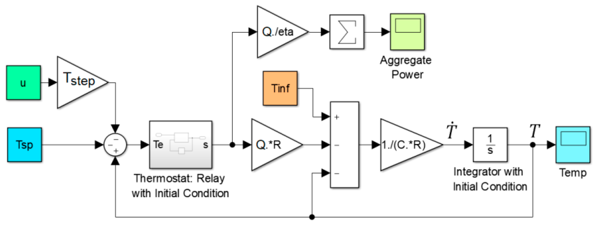
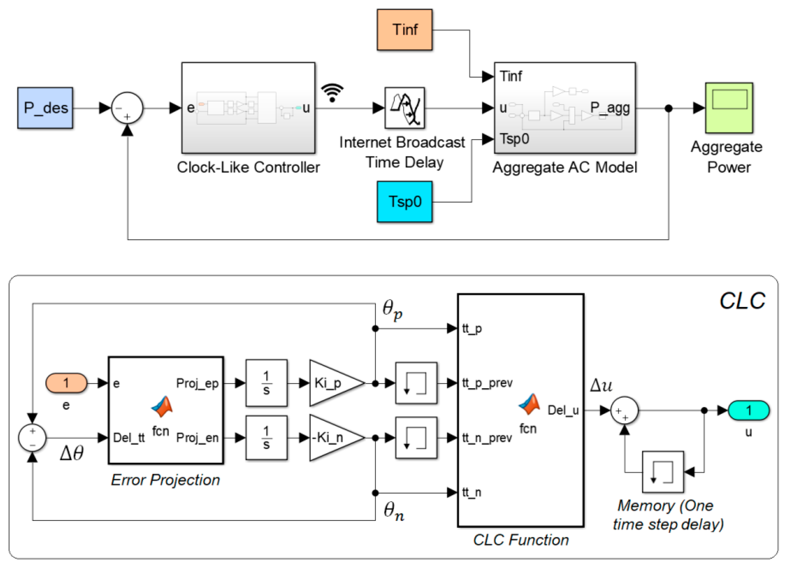
To demonstrate the performance of the proposed CLFC system, a simulation is created, in which the microgrid frequency is controlled using the aggregate AC power only. The block diagram of this hypothetical system is shown in Figure 10. The CLFC subsystem receives the frequency error, computes the setpoint temperature offsets, and broadcasts them to the AC thermostats with a certain time delay. To simulate the system in the pu scale, the aggregate AC power is shifted down by its initial value to start from zero, and is scaled by a conversion factor (pu_c). This factor is set to be 1/(N_ACP_max) in this simulation, where P_max indicates the expected value of the AC electrical power (i.e., 5.6 kW in this paper). The performance of the CLFC is then evaluated by applying a disturbance ΔL and monitoring the frequency error signal.

The simple case of constant ambient temperature (30 °C) is considered for the simulation of this section. The disturbance signal is set to be 5% step increase in load, 1 min after the start of the simulation. For the first simulation, time delay and ε_f are set zero, the value of σ is set 5, and the two integrator gains are set to be equal (i.e., K_i,p = K_i,n). Figure 11 shows the response of the CLFC system for different values of the integrator gains. As can be seen from Figure 11a, the frequency recovery is accomplished successfully, with the frequency returning to the original level after a temporary departure. The larger the integral gains, the smaller the frequency deviation. The integral gain cannot be increased beyond a certain value due to risk of instability because of time delays. Figure 11b shows that the frequency recovery is achieved by moving the AC power in the opposite direction of the load disturbance, and hence, maintaining the power balance in the system. The clock hands separation angle for this simulation are shown in Figure 11c in the pu scale, with 1 pu indicating 2π radians. It is important to note that if the load disturbance is not corrected externally, the clock hand separation will drift toward 1.0 pu, resulting in control saturation and loss of performance.

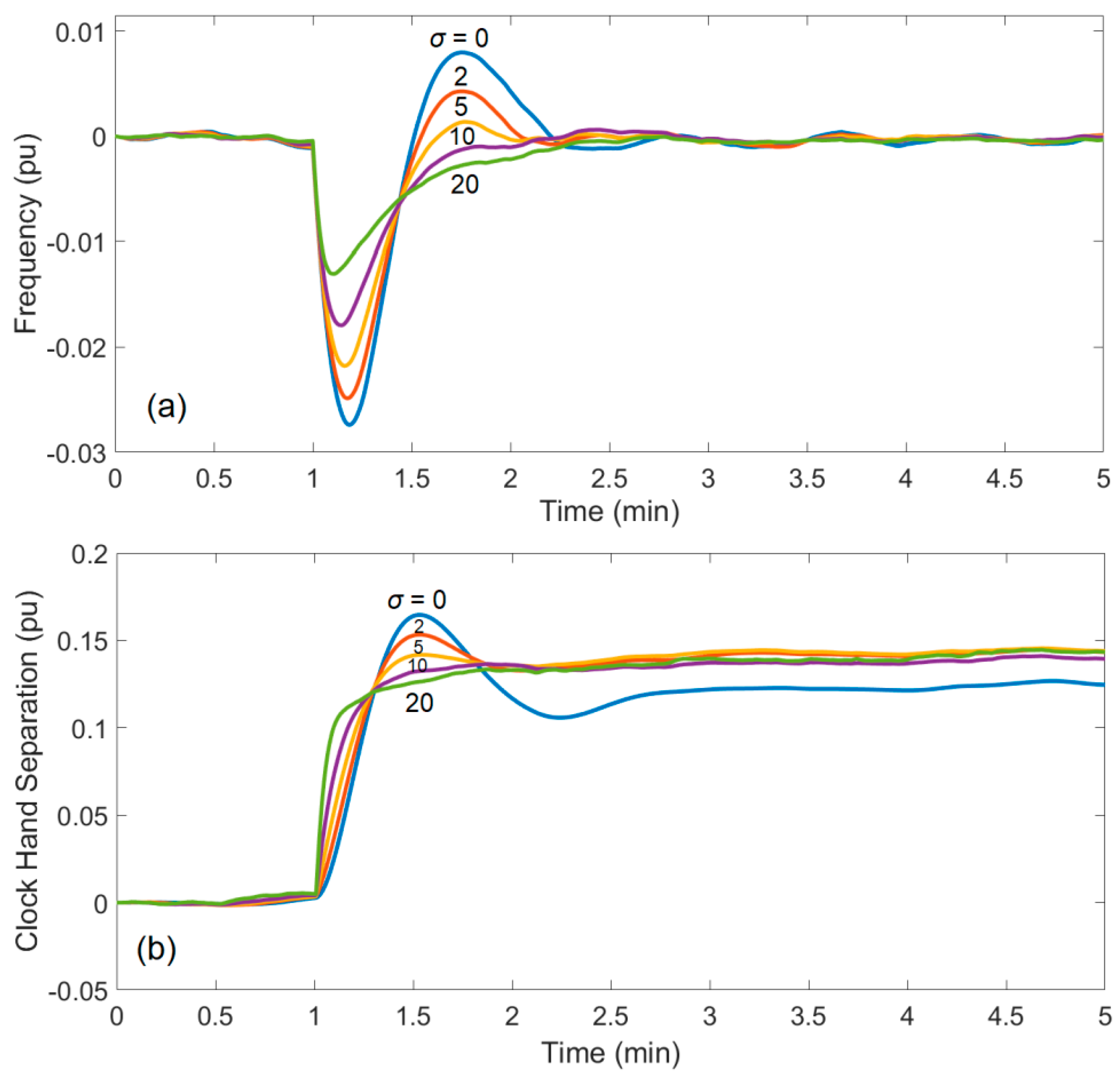
To demonstrate the effects of the frequency time derivative, the same simulation is repeated by fixing the integrator gains (K_i,p = K_i,n = 2) and trying different values of σ, ranging from 0 to 20. Time delay and ε_f are kept at zero. Figure 12 shows the resulting frequency trajectories, underscoring impact of the derivative term in the controller’s transient performance. Although increasing σ enhances frequency error characteristics, it may increase risk of noise amplification. In the simulations of this paper, the value of σ is set to 5 to create a reasonable balance between performance and noise sensitivity in the system.

The next simulation is to evaluate the impacts of time delay. Since internet communication is not delay-free, it is important to evaluate the impacts of different communication delays on the controller performance. Figure 13 shows the performance of the system for different time delay values ranging from 0–10 s. As can be seen, the time delay results in performance drop and possible instability. In practice, an upper bound must be characterized for the time delay, and used to tune the appropriate control gains. The larger the time delay, the smaller must be the CLFC integrator gains. A time delay of 4 s is used in the simulations of this paper, hereafter.

The last simulation of this section investigates the impact of parameter ε_f, the activation threshold for CLFC. Figure 14 shows the response of the system with ε_f = 0.01 pu compared to ε_f = 0. For the nonzero ε_f, the grid frequency remains within ±ε_f, except during the disturbance period around t = 20 min. The maximum frequency deviation is, however, similar to the one with ε_f = 0. It is important to note that in the CLFC formulation, ε_f represents the upper bound of modified error signal (ξ). Figure 14a shows that this parameter can also serve as an upper bound for the frequency error. The clock hands separation angle in Figure 14b indicates that increasing the value of ε_f from 0 to 0.01 reduces the sensitivity of the CLFC considerably, thereby enhancing user comfort without compromising the control performance during fault periods.

4.3. Simultaneous Generation and Demand Control

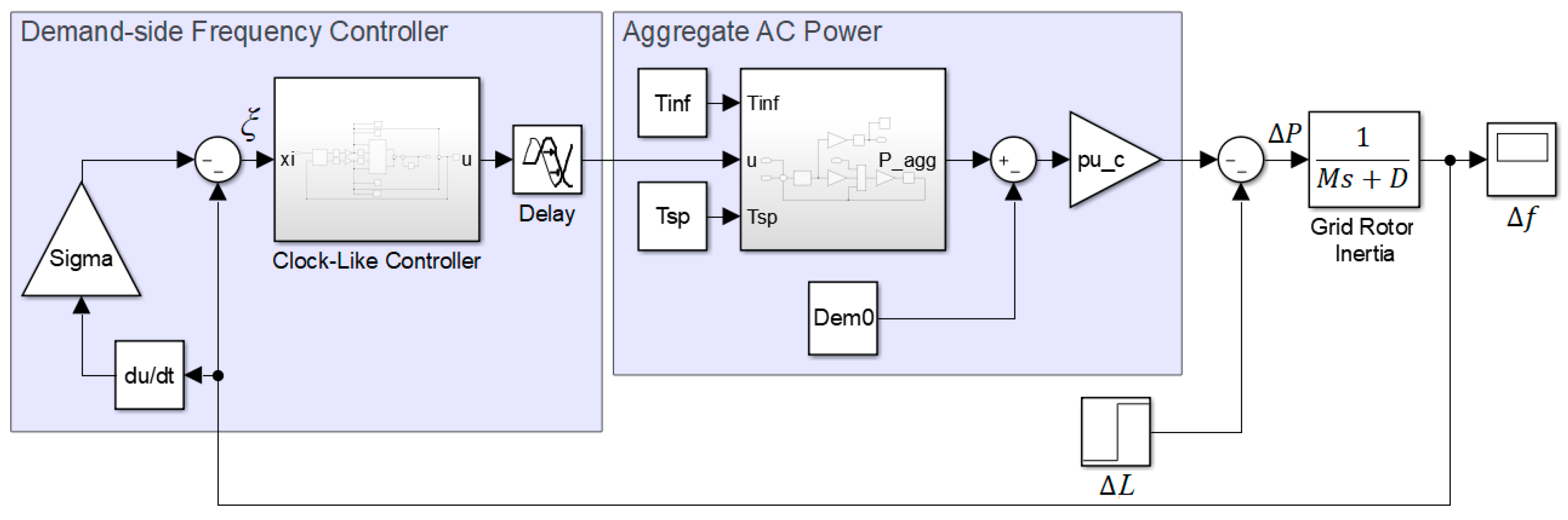
In this section, the demand-side CLFC algorithm is integrated with AGC after some modifications in the AGC system. First, rate limits of 2% and 100% per minute are applied to the steam and the hydro plants, respectively, based on the values suggested in [24]. Moreover, capacity limits of 0.8 pu and 0.2 pu are applied to the steam and the hydro plants to reasonably scale the two power plants and keep their output limited to their maximum value. To further improve the frequency dynamics, a second integrator is added to the steam plant to maintain the integral of the frequency near zero, for maintaining the grid’s clock cycle accuracy. Finally, to avoid integration wind up in the event of rate or capacity saturation, an integrator anti-windup algorithm is applied to both integrators. This logic compares the control signal with the rate and saturation limits, and stops integration during periods when the limits are activated. The full power system diagram with both CLFC and modified AGC system is shown Figure 15. The ambient temperature and the user setpoint inputs are included inside the aggregate AC model subsystem. In addition, a renewable source is included in the simulation.

The initial simulation is for the simple case of constant ambient temperature (30 °C), and a 5% step increase in the demand. The renewable source is set to zero for this simulation. Figure 16a shows the response of the system for four different scenarios: steam plant only, steam and CLFC, steam and hydro, and all three systems together.

When only the steam plant controller is active, the frequency recovery is very slow due to the 2% per min rate limit on the steam plant. In this case, the inclusion of CLFC helps to improve frequency recovery. However, when the hydro plant is included in the control loop, the benefit of CLFC is diminished, since the hydro plant responds quicker than both steam plant and CLFC due to faster ramp rate (100% per minute). Figure 16b shows the outputs of the power plants, the aggregate AC power, as well as the injected load disturbance for the case of having all three systems included in the control loop. The hydro power plant responds to the load immediately, and then drops gradually as the steam plant overtakes the load. The aggregate AC power truncates about a quarter of the load disturbance and maintains its state within the 10 min simulation interval. In the extended simulation, however, the aggregate AC power returns to its initial state through the setpoint correction mechanism built in the CLFC algorithm.

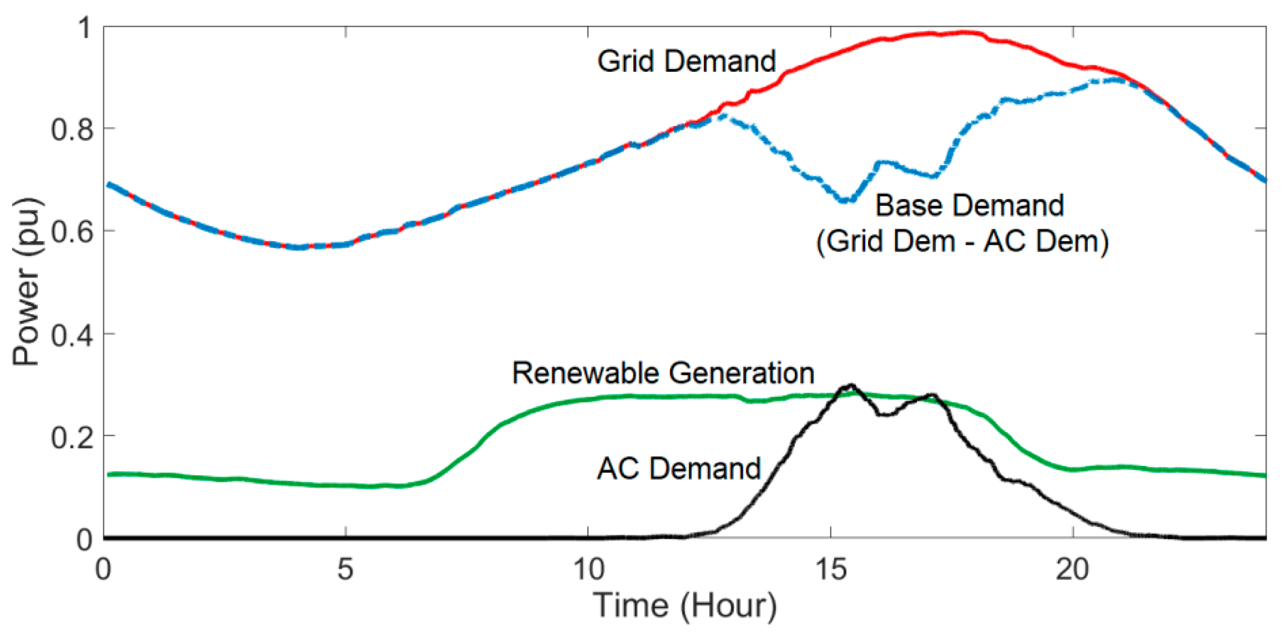
The previous simulation reveals that the CLFC system can be outpaced by the hydro plant under normal conditions. In the next section, a scenario is investigated, in which the power demand exceeds the maximum generation capacity of the microgrid. This can happen on a very hot day, when the AC units work excessively to maintain desirable indoor temperatures. To provide a realistic simulation, the ambient temperature shown in Figure 2 is shifted up by 5 °C to resemble a hot day with 22 °C low and 37 °C peak temperature. The California Independent System Operator (CAISO) data is used to obtain sample grid demand and renewable power profiles for the simulation. The data for the same day as the ambient temperature data is used for consistency. To separate the aggregate AC power from the total grid demand, the true ambient temperature is used first to obtain and subtract the aggregate AC power from the demand. To covert the power data to the pu scale, a margin of 2% is assumed for the peak demand below the generation capacity (combined steam and hydro). The net demand, defined as the total power demand minus renewable power, has a much larger clearance margin from the generation capacity (around 30%).

Figure 17 shows the resulting power trajectories. The peak aggregate AC power is around 30% of the total grid demand for the true ambient temperature. This value would rise to around 59% when the ambient temperature is offset by 5 °C. The base demand (dashed line in Figure 17), defined as the total grid demand minus the aggregate AC power, is used as the demand input in the simulation, with aggregate AC power being calculated via CLFC, and injected to the system separately.

It is important to note that all the power inputs (AC, base demand, and renewable) are offset to start from zero in the simulation to avoid initial imbalance in the system. The steam and hydro plant saturation limits are offset as well to account for these initial conditions. The hydro plant is assumed to be in its mid-point, initially, moving the saturation limits from [0 0.2] to [−0.1 0.1], and the rest of the load minus the renewable generation is initially picked up by the steam plant.

Figure 18 shows the simulation results with and without CLFC, for the case of elevated ambient temperature. As can be seen in Figure 18a, in the absence of CLFC, the frequency deviates significantly during certain time periods. The reason is that the net demand (total power demand minus renewable power) exceeds the maximum generation capacity as shown in Figure 18b, resulting in the saturation of both steam and hydro power plants. The integrator anti-windup plays a crucial role in the timely recovery of frequency after the net demand returns to the trackable range. To maintain the clock cycle accuracy, there is an over-frequency period (between Hours 20–30), during which the integral of frequency is corrected to zero. The integrator gain for this purpose, i.e., K_i,G2, is set to 0.0001. Note that, the simulation time is extended to 36 h (repeating the first 12 h) for a better view of the system responses.

When the CLFC mechanism is active, the frequency deviation is maintained within ±ε_f (0.005 pu). This is achieved by curtailing the aggregate AC power such that the net grid demand remains below the generation capacity, as seen in Figure 18c. The clock hands separation angle in Figure 18d shows how CLFC responds to the frequency error. When the error is within the specified limit, the frequency control is accomplished by the steam and the hydro plants, and the clock hands are locked unless separation angle is nonzero. When the frequency approaches the threshold limits due to AGC saturation, the CLFC takes action automatically to contain the frequency within the specified range. Clock hand separation angle returns slowly to zero when |ξ| < ε_f, via the setpoint correction mechanism. The value of α is set to 0.0001/2π in this simulation.

Evaluating the total simulation time for the simultaneous AGC and CLFC system with 5000 AC units indicates that the proposed CLFC method is a computationally-friendly algorithm. It takes around 3 milliseconds per simulation time step to compute both control signals and the evolution of AC temperatures using a computer with 8 GB memory and an Intel Core i7 processor. The proposed control method can therefore accommodate millions of AC systems for large-scale grid-wide updates every 2–4 s. The main limitation remains to be the internet communication bandwidth and delays associated with broadcasting control signals to the connected thermostats.

The simulations of this section underscore the importance of demand-side energy management in resource limited microgrids when the conventional generation system reaches its maximum capacity. This research can be extended to investigate other scenarios such as presence of energy storage, economic load dispatch, and larger power grids with multi-area networks.

5. Conclusions

This paper proposed a novel control method for demand-side energy management in microgrids through internet-connected smart thermostats. The advantage of the proposed clock-like control framework is providing smooth power demand control by offsetting setpoint temperatures of loads at discrete intervals, within the capability of thermostats, in a systematic (non-random) manner. The formulation of the clock-like controller for power tracking and frequency control in microgrids was presented and evaluated through various simulations. The proposed controller is able to achieve tracking of desired power trajectories, as well as limiting the peak demand under a certain threshold, with a reasonable accuracy. The frequency control simulations indicated that proposed controller is able to stabilize the grid frequency by itself and in cooperation with generation control. In the presence of fast power plants, however, the impact of demand-side controller is diminished due to time delays in the communication network as well as the internal dynamics of the loads. The demand-side frequency controller provides an additional security margin in scenarios where the power demand exceeds the maximum generation capacity of the microgrid due to unusual weather conditions and contingences. A robust internet communication network between the grid operator and the thermostats, with a predictable time delay upper bound, is a key to the successful tuning and implementation of the proposed control method.