Data-Driven Framework to Predict the Rheological Properties of CaCl₂ Brine-Based Drill-in Fluid Using Artificial Neural Network

Abstract

Calcium chloride brine-based drill-in fluid is commonly used within the reservoir section, as it is specially formulated to maximize drilling experience, and to protect the reservoir from being damaged. Monitoring the drilling fluid rheology including plastic viscosity, $PV,$ apparent viscosity, $AV,$ yield point, $Y_p,$ flow behavior index, $n,$ and flow consistency index, $k,$ has great importance in evaluating hole cleaning and optimizing drilling hydraulics. Therefore, it is very crucial for the mud rheology to be checked periodically during drilling, in order to control its persistent change. Such properties are often measured in the field twice a day, and in practice, this takes a long time (2–3 h for taking measurements and cleaning the instruments). However, mud weight, $MW$, and Marsh funnel viscosity, $MF$, are periodically measured every 15–20 min. The objective of this study is to develop new models using artificial neural network, ANN, to predict the rheological properties of calcium chloride brine-based mud using $MW$ and $MF$ measurements then extract empirical correlations in a white-box mode to predict these properties based on $MW$ and $MF$. Field measurements, 515 points, representing actual mud samples, were collected to build the proposed ANN models. The optimized parameters of these models resulted in highly accurate results indicated by a high correlation coefficient, R, between the predicted and measured values, which exceeded 0.97, with an average absolute percentage error, AAPE, that did not exceed 6.1%. Accordingly, the developed models are very useful for monitoring the mud rheology to optimize the drilling operation and avoid many problems such as hole cleaning issues, pipe sticking and loss of circulation.

1. Introduction

Drilling Fluids are considered a key element in the drilling operation. Conventional drilling fluids are water-based, oil-based or synthetic-based fluid systems, which are used in the drilling process to give the best performance under certain temperatures and pressures experienced downhole [1]. Drilling the section from the sea-bed/land to the top of the reservoir is different, regarding the economic value of the final project, compared to the reservoir section. As in the top sections, the concerns are to seal the permeable formations, and help sustain the wellbore stability.

Special measures will be taken into consideration while drilling the reservoir section to avoid damaging the reservoir and plugging the reservoir pores. For that target, special drilling fluids are used, called reservoir drill-in fluids (RDFs), which are specially formulated to maximize drilling experience and protect the reservoir from being damaged until the completion process is proceeded [2].

There are many types of RDFs with different chemical compositions, but the concern of this study is about the clear brine-based mud which is often used within completions, as the presence of solids is a major contributor to formation damage [3]. However, when used as drilling fluid, the solids-free nature of brine operationally improves the rate of penetration (ROP), stabilization of sensitive formations, density, and abrasion or friction [4]. Clear brine fluids properties are easier to maintain than conventional solids-laden fluid systems, so that when properly run, clear systems require very little maintenance, because many functional issues are inherently solved by the dissolved salts. Clear brine fluids also allow for drill site cost reductions because of the ability to reuse the fluid [5].

Brine fluids can be prepared with one salt or a combination of salts. All salts provide unique properties to the base fluid. Saturated brines fluids provide excellent inhibitive properties and lubricity, as compared to conventional aqueous fluids. With optimal heat transference characteristics, they can greatly improve bit life, and increase the rate of penetration in hard rock drilling. Among the different salts used for clear-brine systems, calcium chloride has been selected, as it is considered one of the most economic brine systems, with its broad range of densities (from 9.0 to 11.6 ppg), availability, low cost, and its ability to reduce the water activity of the fluid [6].

1.1. Drilling Fluid Rheology

Drilling fluid rheology plays a key role in optimizing drilling performance [7]. These properties significantly affect the efficiency of the hole cleaning and the drilling rate [8], which are critical factors controlling the performance of drilling operation [9]. These rheological properties include mud density to provide the control on the formation pressure, while $PV, Y_P, AV, n$ and $k$ are used for controlling hole cleaning and optimizing the drilling performance [10]. Plastic viscosity of the drilling fluid is crucial for optimizing the drilling operation [11]. It is an indication of the solid content in the drilling fluid which may negatively affect the drilling performance when it exceeds critical limits, and can cause many problems like pipe sticking and decreasing the rate of penetration [12]. Yield point can be simply stated as the attractive forces among colloidal particles in drilling fluid [11]. The optimization of yield point is central to controlling the efficiency of hole cleaning [10,13]. Moreover, apparent viscosity is considered a key factor in the optimization of mud hydraulics while drilling [8]. In addition, the parameters k and n can be used for evaluating hole cleaning during the drilling operation [14].

The rheological properties can be measured in the laboratory using mud balance and viscometer. The mud balance is used to measure the mud weight while the rheometer is used to measure ($PV, Y_P, AV, n$ and $k$). However, this process takes a relatively long time (2–3 h for taking measurements and cleaning the instruments) which makes it difficult to be performed periodically and practically in the field. Therefore, it is taken as a common procedure that only density and Marsh funnel viscosity are measured periodically every 15–20 min, using mud balance and Marsh funnel devices. On the other hand, a complete mud test (including all the drilling fluid properties), using the mud balance and viscometer, is performed twice a day. Marsh funnel viscosity provides an indication of the changes in the rheology of the drilling fluid. This funnel was first introduced by Marsh [15]. 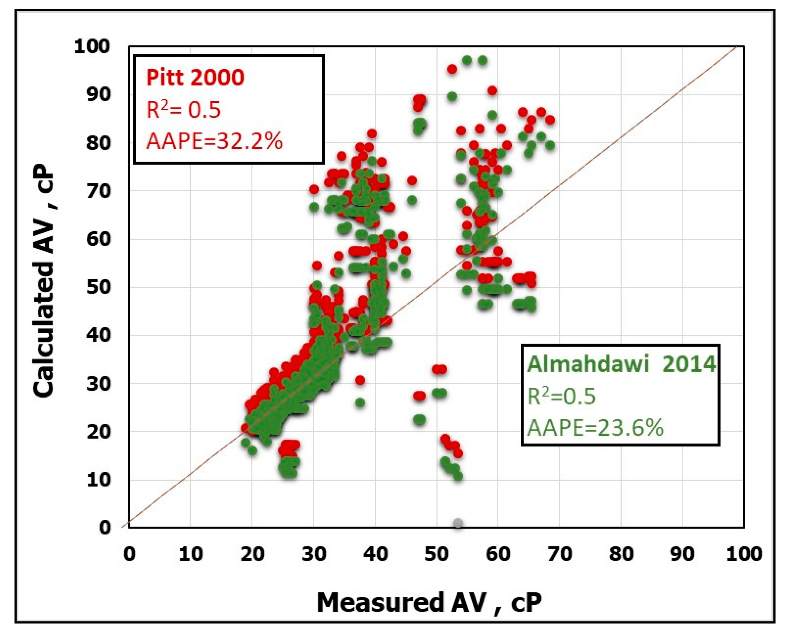This tool is cheap and takes a short time, so it can be utilized to give field measurements frequently and estimate some parameters like yield stress [16]. Based on the literature, there are two models developed to predict the drilling fluid viscosity from mud density and Marsh funnel measurements. These two measurements were used as inputs to calculate the effective viscosity of the drilling fluid as stated by Pitt [17] in Equation (1). Then a modification on the previous model was introduced by Almahdawi et. al. [18], who figured out that changing the value of the constant to 28 in Equation (2) instead of 25 presented by Pitt [17], is more effective give more accurate results, as compared to Equation (1).

$$AV=D(T-25)$$

(1)

$$AV=D(T-28)$$

(2)

where $AV$ is the apparent viscosity in cP, $D$ is the fluid density in $g/c{m}^3$, $T$ is the Marsh funnel time in sec.

Several mathematical models have been mentioned in the literature for estimating the fluid rheological properties using Marsh funnel devices. Some of them suggested using the temporal variations in the fluid height in the funnel to determine different rheological parameters such as $PV, Y_P \mathrm{and}AV$ [19,20,21,22]. They introduced a methodology to determine the shear rate and the shear stress on the walls of the Marsh funnel from the measured discharged fluid volume of the Marsh funnel at different points. Then several rheological parameters have been related to the obtained shear rate and shear stress. Abdulrahman et al. [23] investigated different water-based drilling fluids using the Marsh funnel and showed that $PV \mathrm{and}AV$ can be estimated using consistency plots and the methodology described in [19]. However, these models showed considerable discrepancies between the results obtained from the Marsh funnel and the standard viscometers. Other studies tried to model the fluid volume flow in the Marsh funnel with higher order polynomial functions, rather than the simplified functions used in the previously mentioned studies [24,25]. This attempt was to simulate the fluid temporal height in the Marsh funnel more properly, and to get closer results of rheological parameters to those obtained from the standard viscometers.

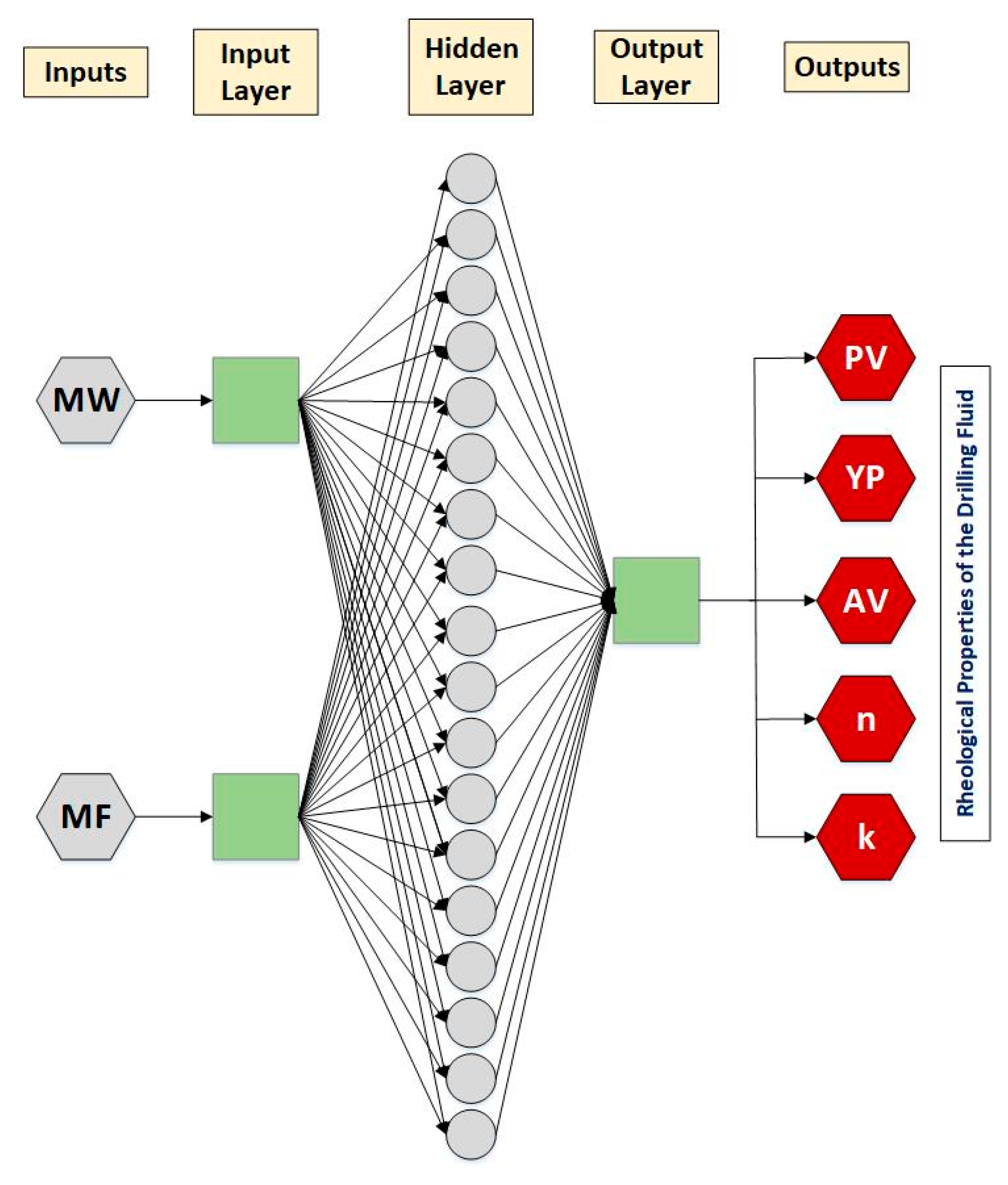
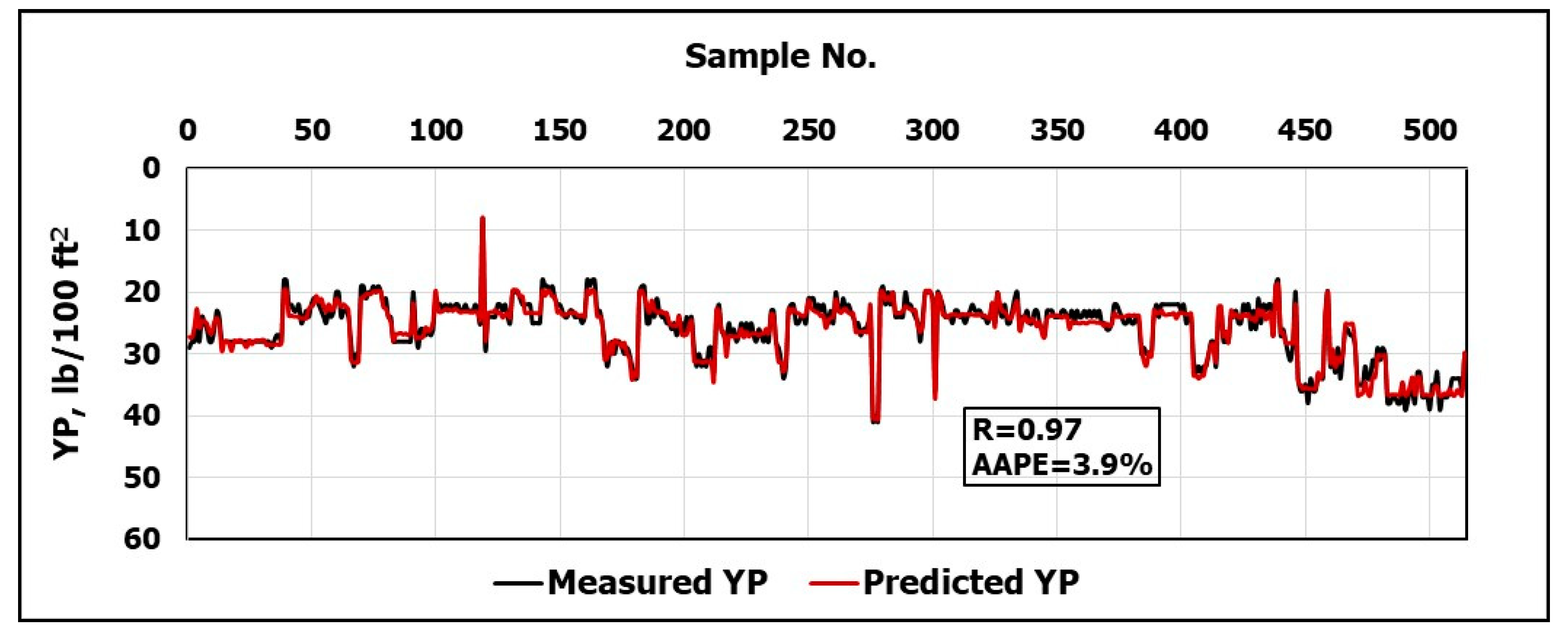
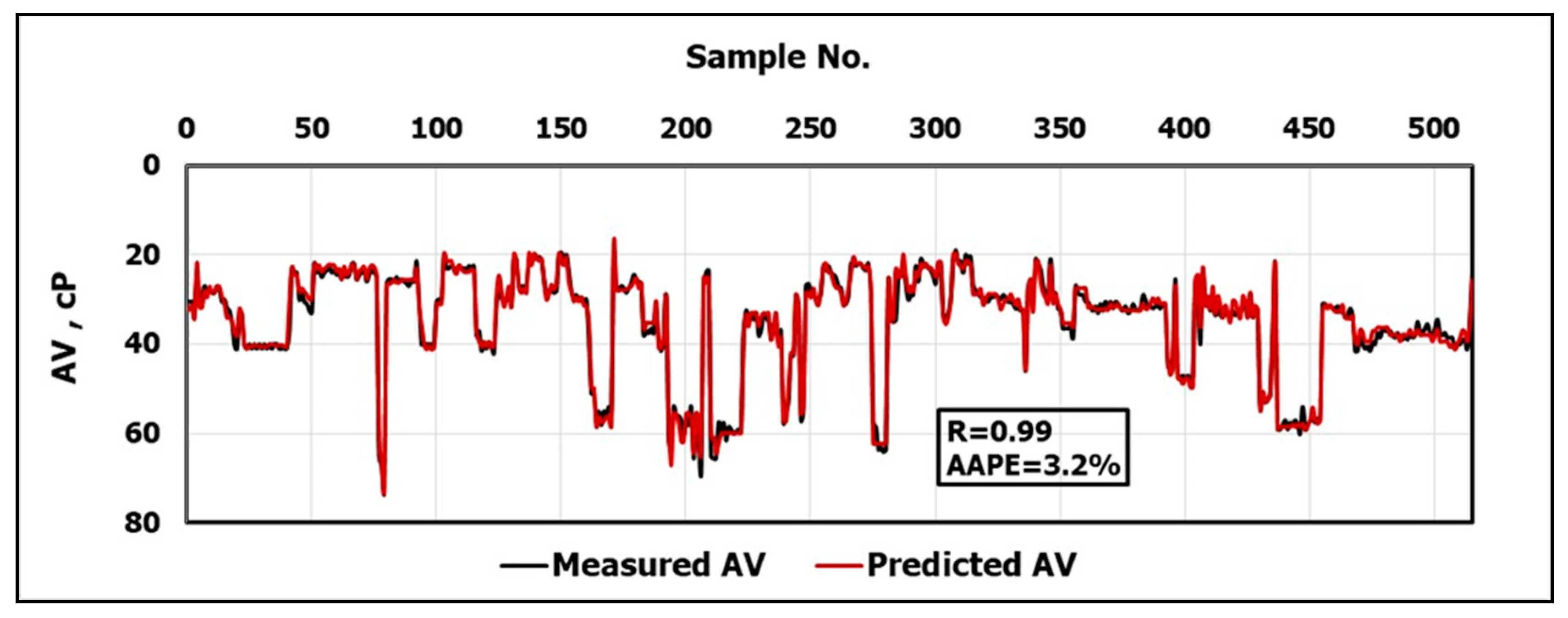
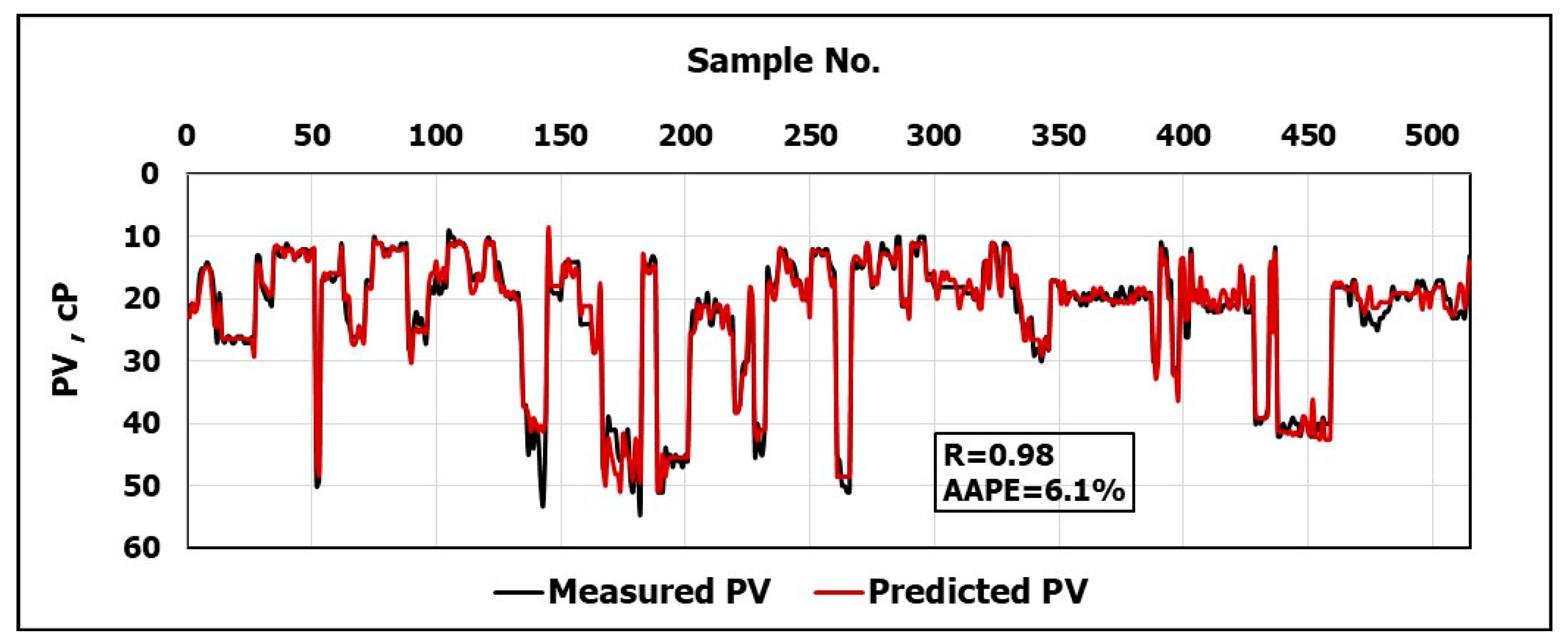
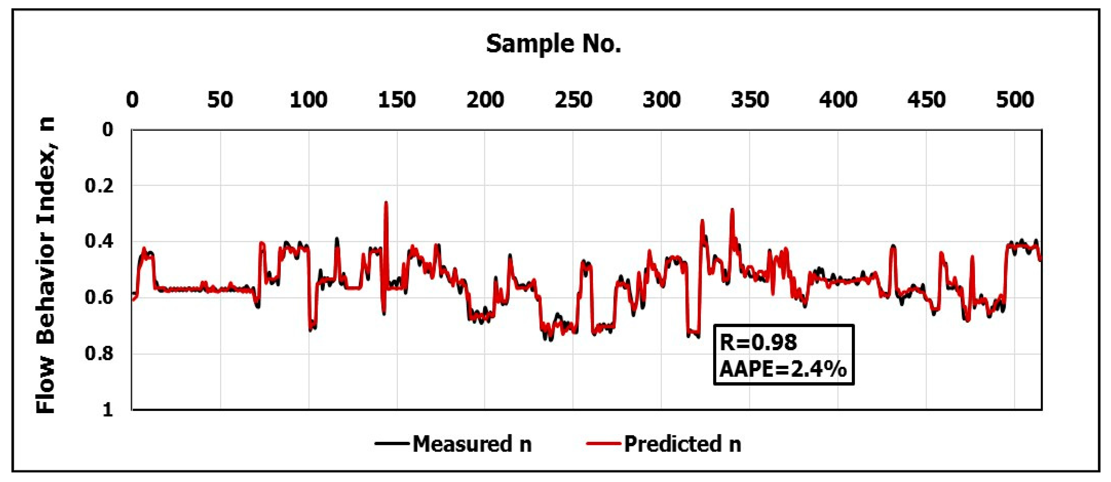
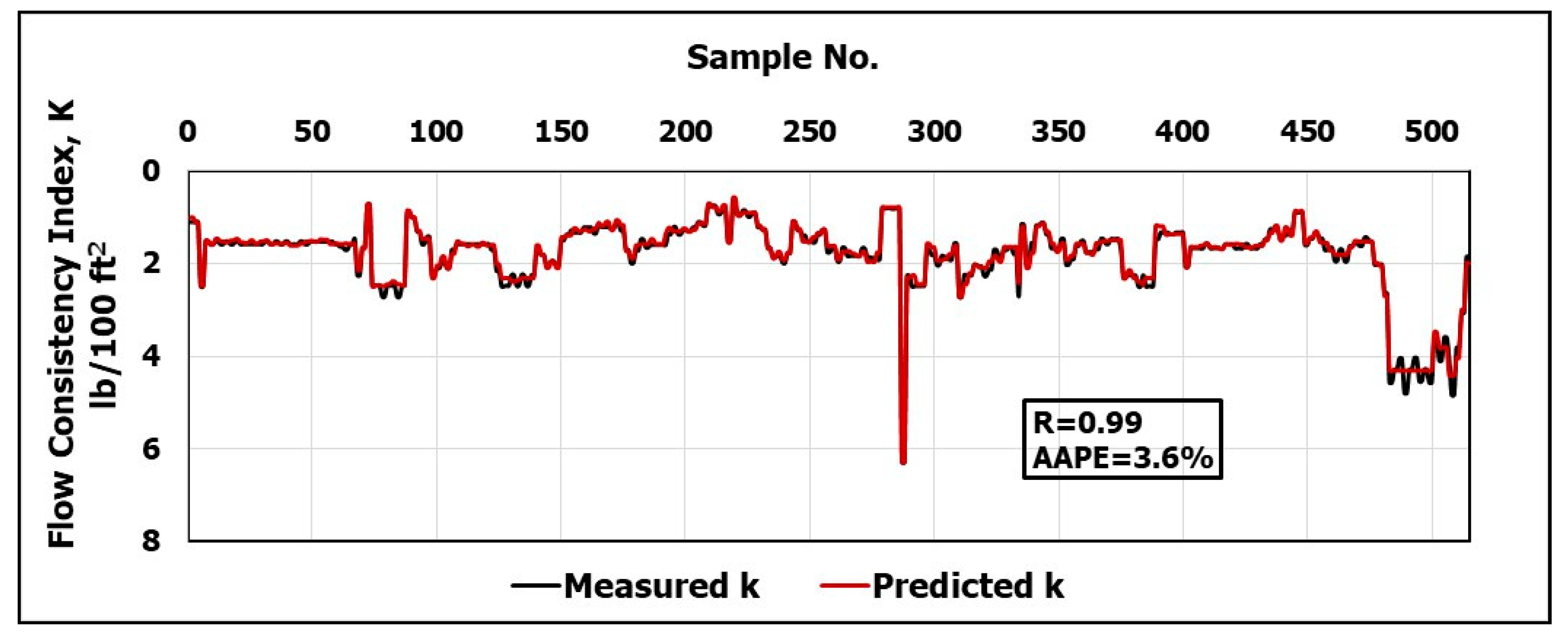
The objective of this work is to develop new models using artificial neural networks, ANN, to predict the rheological properties of the CaCl₂ brine-based drilling fluid depending on frequent measurements of $MW$ and $MF$. The real-time measurements of these parameters are very helpful for identifying the efficiency of the hole cleaning, optimizing the drilling fluid hydraulics, equivalent circulating density calculations and swab and surge pressure determination.

1.2. Artificial Neural Network (ANN)

Artificial intelligence, (AI), can be simply defined as the computer science branch for creating intelligent machines [26] to exhibit human brains to make predictions and help take the right decisions for the future scenarios [27]. Recently, different AI methods such as fuzzy logic, FL, support vector machine, SVM, genetic algorithm and artificial neural network, ANN, have been applied in petroleum engineering, and specifically in the field of drilling fluid engineering. Some of these applications include fluid flow patterns prediction in wellbore annulus [28], stuck pipe prediction [29], drilling hydraulics optimization [30], frictional pressure loss estimation [31], hole cleaning and prediction of cutting concentration [32], estimation of the static Poisson’s ratio from log data [33].

ANN is one of the most common AI techniques which has the ability to deal with different engineering problems with high complexity that exceed the computational capability of classical mathematics and procedures [34]. It is based on analogy with biological neural networks to simulate the performance of the human biological neural system [35]. The elementary units for ANN are neurons [36]. The structure of the ANN consists of three main types of layers. The first one is for the input parameters. The second one is called hidden layers, which include the neurons assigned with the transfer functions between the inputs and the outputs. The third type is for the outputs. These layers, with the suitable training algorithm, describe the nature of the problem [37]. The performance of the network is controlled by key parameters including the number of neurons, weights and biases [38]. To optimize the weight and biases, the network is trained using different algorithms to achieve the lowest possible error. Among these algorithms is Levenberg-Marquardt (LM), which is an iterative, curve fitting algorithm. This algorithm proved its outstanding performance in solving non-linear least-squares problems [39].

There are many ANN applications of ANN in the field of drilling fluid in the last few years. Some of these researches are the prediction of filtration volume and mud cake permeability of water-based mud (WBM) [40], drill cutting settling velocity prediction [41], prediction of differential pipe sticking [42], lost circulation prediction [43], hole cleaning efficiency of foam fluid [44], rheological properties of invert emulsion mud [45], invert emulsion mud rheology [46] and spud mud rheology prediction [47], generating geomechanical well logs [48], prediction of oil PVT properties [49].

Based on the literature, more than 50 percent of the applications in the drilling fluid area used ANN for the predictions and got high accurate results. Accordingly, ANN has been selected for building the proposed models in this study [26].

2. Methodology

2.1. Data Description

A typical sample of the data for CaCL₂ brine-based drill-in fluid (515 field data for actual mud samples) is listed in

Table 1. A typical sample of the CaCl₂ brine-based drilling fluid collected data.

$\mathit{M}\mathit{W}, \mathit{I}\mathit{b}/\mathit{f}{\mathit{t}}^3$	$\mathit{M}\mathit{F}, \mathit{s}/\mathit{q}\mathit{u}\mathit{a}\mathit{r}\mathit{t}$	$\mathit{P}\mathit{V}, \mathit{c}\mathit{P}$	${\mathit{Y}}_{\mathit{P}}, \mathit{I}\mathit{b}/100 \mathit{f}{\mathit{t}}^2$
78	62	8	21
80	45	8	22
88	62	12	18
73	50	11	20
65	48	11	21
75	44	12	20

, including $\left(MW, MF, PV, \mathrm{and} Y_p\right)$. The drilling fluid samples are collected after the mud was cleaned from the cuttings by using the shale shaker $MW$ and $MF$ are measured in the field using a mud balance and Marsh funnel, respectively. The rheometer is used for measuring the rheology of the mud, namely $PV, \mathrm{and} Y_p$ at atmospheric pressure and ${120}^{o}F$. The collected data have a wide range as follows: $MW$ ranges from 43 to 119 $Ib/f{t}^3$, $MF$ ranges from 26 to 135 $s/quart$, $PV$ ranges from 10 to 54 cP, and $Y_P$ ranges from 8 to 41 $Ib/100 f{t}^2$. Figure 1 shows that $MW$ has R of 0.36 and 0.76 with $Y_P$ and $PV$ respectively while $MF$ has R of 0.86 with $Y_P$ and 0.36 with $PV$.

For better prediction using AI models, data should be analyzed and filtered [50]. Therefore, the selected data have been cleaned from any noise and false values for higher representation quality. The filtration process included eliminating all the values that cannot be representative, like negative values. Finally removing the outliers that show significant deviation from the other values of a variable, the outliers were removed using a box and whisker plot, in which top whisker represents the upper limit of the data, and the bottom whisker represents the lower limit of the data, then any value beyond these limits is considered an outlier and removed [51]. These limits are determined by dividing the data into four equal divisions (quartiles) along with using the minimum, maximum, mean and median parameters [52] obtained from the statistical analysis of the data listed in

Table 2. Statistical Analysis of the CaCl₂ brine-based mud collected data.

Parameter	$\mathit{M}\mathit{W}, \mathit{I}\mathit{b}/\mathit{f}{\mathit{t}}^3$	$\mathit{M}\mathit{F}, \mathit{s}/\mathit{q}\mathit{u}\mathit{a}\mathit{r}\mathit{t}$	$\mathit{P}\mathit{V}, \mathit{c}\mathit{P}$	${\mathit{Y}}_{\mathit{P}}, \mathit{I}\mathit{b}/100 \mathit{f}{\mathit{t}}^2$
Min.	43	26	10	8
Max.	119	135	54	41
Mean	85.45	56.33	22.59	25.88
Mode	76	109	44	33
Range	72	50	19	24
Skewness	0.50	1.43	1.29	0.83

.

2.2. Development of ANN Models

The collected data were used to calculate $R_{600}$ and $R_{300}$ (rheometer readings at 600 and 300 rpm, respectively) using Equations (3) and (4). These two parameters are very crucial for identifying fluid properties and flow regimes. Then, the apparent viscosity, $AV$, flow behavior index, $n$, and flow consistency index, $k$, are calculated using Equations (5)–(7) respectively.

$$R_{600}=P_V+R_{300}$$

(3)

$$R_{300}=P_V+Y_p$$

(4)

$$AV=\frac{R_{600}}{2}$$

(5)

$$n=3.32\times \log \left(\frac{R_{600}}{R_{300}}\right)$$

(6)

$$k=\frac{R_{600}}{{1022}^n}$$

(7)

For all the upcoming developed models, different scenarios have been performed to optimize the ANN variables to reach the highest accuracy with the lowest possible error for prediction using different combinations of the available options of the ANN variables. The optimized parameters obtained from the tuning process of these parameters are summarized in

Table 3. Summary of the optimized parameters for the developed ANN models.

Neural Network Parameter	Types and Range
Training Algorithm	Levenberg Marquardt
Number of neurons	20
Number of hidden layer(s)	1
Learning rate	0.12
The hidden layer transfer function	Tan-sigmoidal
The outer layer transfer function	Pure-linear
Training ratio	70%
Testing ratio	30%

. The chosen architecture for the developed models includes three layers:

–

Input layer: It contains input features which are $MW$ and $MF$.

–

(One) Hidden layer: It contains the optimized number of neurons which was found to be 20 neurons.

–

Output layer: It contains the output parameters, which are ($PV, Y_P, AV, n$ and $k$ individually).

The network was trained using the Levenberg-Marquardt (LM) algorithm to get the optimized weights and biases. The neurons are arranged to be trained using a learning rate of 0.12. Activation function of the tan-sigmoidal type (tansig) was assigned between the input and hidden layers while the pure-linear function was assigned between the hidden and output layers. Figure 2 shows a typical schematic of the architecture of the developed ANN model.

3. Results and Discussion

3.1. Yield Point ($Y_P$) Model

An ANN-Based model was developed using $MW$ and $MF$ as inputs to predict the $Y_P$ values. The obtained data were divided into ratios 70:30 for training and testing the model, respectively. Figure 3 shows the high match between the measured and the predicted $Y_P$ values from the developed ANN model in terms of R of 0.97 and AAPE of 3.9%. Thereafter, a new correlation has been developed using the ANN model to predict $Y_P$ based on $MW$ and $MF$. First, the inputs should be normalized using Equations (8) and (9) to substitute the values $M{W}_n$ and $M{F}_n$ in Equation (10); where $M{W}_n$ refers to the first normalized input, and $M{F}_n$ refers to the second normalized input.

$$M{W}_n=0.036(MF-64)+1$$

(8)

$$M{F}_n=0.133(MF-26)+1$$

(9)

Then, the normalized value $Y_P{}_n$ is calculated using Equation (9) with its optimized coefficients listed in

Table 4. The optimized coefficients for estimating the normalized $Y_P{}_n$ in Equation (10).

Neuron Index	Input Layer Weights		Hidden Layer Weights	Input Layer Biases	Output Layer Bias
$i$	$w_{1_{i,1}}$	$w_{1_{i,2}}$	$w_{2,i}$	$b_{1,i}$	$b_2$
1	−4.251	5.585	−0.950	5.530	−0.508
2	−0.709	−6.857	−0.155	4.936	-
3	2.631	5.539	0.168	−4.752	-
4	−0.743	6.411	1.005	3.899	-
5	−4.986	5.903	−0.932	3.661	-
6	−5.203	−0.250	−1.022	3.135	-
7	4.859	4.645	−0.410	−2.792	-
8	−1.185	−6.192	0.721	2.879	-
9	4.188	−3.646	−1.697	−3.015	-
10	3.238	−5.080	0.297	−0.585	-
11	0.708	−7.849	−0.380	0.213	-
12	−4.893	−9.220	−0.428	−1.489	-
13	2.227	−6.971	−1.173	2.051	-
14	3.101	5.504	−1.046	1.840	-
15	−6.059	−1.558	−0.030	−3.063	-
16	−5.020	3.702	−0.902	−3.873	-
17	2.892	5.503	−0.260	4.287	-
18	−0.736	−5.668	0.190	−5.818	-
19	4.290	−4.592	0.639	5.571	-
20	−4.290	4.570	−0.686	−6.252	-

.

$$Y_{P_n}=\left[{\displaystyle \sum _{i=1}^N{w}_{2,i}}\left(\frac{2}{1+\exp \left(-2\left(M{W}_n\times w_{1_{i,1}}+M{F}_n\times w_{1_{i,2}}+b_{1,i}\right)\right)}-1\right)\right]+b_2$$

(10)

where i is the index of the neuron in the hidden layer, N is the optimized number of neurons for only one hidden layer, which is found to be $20$, $w_1$ is the weight vector linking the input and the hidden layer, $w_2$ is the weight vector linking the hidden and output layer, $b_1$ is the biases vector for the input layer, and $b_2$ for the output layer.

Finally, the required $Y_P$ value can be obtained by denormalizing $Y_P{}_n$ using Equation (11).

$$Y_p=16.5\left(Y{p}_n+1\right)+8$$

(11)

3.2. Apparent Viscosity ($AV$) Model

Similarly, $AV$ was predicted using ANN, based on $MW$ and $MF$. The model was trained using 70% of the available data, while 30% of the data were used for testing the model. Figure 4 shows the high R between the predicted and the measured $AV$ values, which is 0.99 with AAPE of 3.2%. Afterward, a new correlation for predicting $AV$ was extracted from the developed ANN model. To use this correlation, the inputs should be normalized at first using Equations (12) and (13) to substitute the values $M{W}_n$ and $M{F}_n$ in Equation (14); where $M{W}_n$ refers to the first normalized input, and $M{F}_n$ refers to the second normalized input.

$$M{W}_n=0.036(MF-64)+1$$

(12)

$$M{F}_n=0.053(MF-35)+1$$

(13)

Then, the normalized value $A{V}_n$ is calculated using Equation (14) with its optimized coefficients listed in

Table 5. The optimized coefficients for estimating the normalized $A{V}_n$ in Equation (14).

Neuron Index	Input Layer Weights		Hidden Layer Weights	Input Layer Biases	Output Layer Bias
$i$	$w_{1_{i,1}}$	$w_{1_{i,2}}$	$w_{2,i}$	$b_{1,i}$	$b_2$
1	2.960	7.136	−0.950	−5.667	1.535
2	−5.586	−7.703	−0.155	2.751	-
3	4.037	5.355	0.168	−1.886	-
4	−3.362	3.743	1.005	2.292	-
5	6.295	−5.066	−0.932	−8.110	-
6	0.406	7.091	−1.022	6.492	-
7	−10.26	−8.654	−0.410	−0.995	-
8	−0.572	−9.022	0.721	−0.909	-
9	−7.565	4.329	−1.697	4.884	-
10	−4.256	3.855	0.297	2.094	-
11	6.458	1.765	−0.380	1.786	-
12	4.537	−4.152	−0.428	1.324	-
13	−5.410	3.103	−1.173	−2.553	-
14	−4.859	−2.202	−1.046	−1.924	-
15	−7.190	1.704	−0.030	−4.783	-
16	2.196	−5.993	−0.902	2.408	-
17	−0.576	6.113	−0.260	−4.569	-
18	−2.889	−4.782	0.190	−4.645	-
19	−3.799	−7.588	0.639	−2.337	-
20	−3.877	4.861	−0.686	−6.301	-

.

$$A{V}_n=\left[{\displaystyle \sum _{i=1}^N{w}_{2,i}}\left(\frac{2}{1+\exp \left(-2\left(M{W}_n\times w_{1_{i,1}}+M{F}_n\times w_{1_{i,2}}+b_{1,i}\right)\right)}-1\right)\right]+b_2$$

(14)

Finally, $AV$ can be predicted by denormalizing $A{V}_n$ using Equation (15).

$$AV=27\left(A{V}_n+1\right)+19$$

(15)

3.3. Plastic Viscosity ($PV$) Model

For $PV$, another ANN model was developed based on $MW$ and $MF$. For building the model, the ratio of the training to testing points is 70:30. The model gave high accurate results indicated by a high R of 0.98 between the predicted and the measured $PV$ values and maximum AAPE of 6.1% as shown in Figure 5. A new correlation has been extracted from the model to predict $PV$ without the need to run the ANN model.

First, the inputs should be normalized using Equations (16) and (17) to substitute the values $M{W}_n$ and $M{F}_n$ in Equation (18); where $M{W}_n$ refers to the first normalized input, and $M{F}_n$ refers to the second normalized input.

$$M{W}_n=0.037(MF-64)+1$$

(16)

$$M{F}_n=0.105(MF-35)+1$$

(17)

Then, the normalized value $P{V}_n$ is calculated using Equation (18) with its optimized coefficients listed in

Table 6. The optimized coefficients for estimating the normalized $P{V}_n$ in Equation (18).

Neuron Index	Input Layer Weights		Hidden Layer Weights	Input Layer Biases	Output Layer Bias
$i$	$w_{1_{i,1}}$	$w_{1_{i,2}}$	$w_{2,i}$	$b_{1,i}$	$b_2$
1	−3.740	4.001	1.983	9.616	−1.831
2	−3.304	−5.296	−1.243	−5.482	-
3	−11.57	−3.788	3.380	7.537	-
4	−6.403	−2.376	−4.833	4.301	-
5	1.308	7.156	−0.307	2.069	-
6	0.457	−12.03	1.182	1.413	-
7	−3.684	10.384	−0.141	3.236	-
8	1.511	−3.887	1.414	−3.601	-
9	−7.490	−1.848	1.788	6.460	-
10	−5.945	−6.028	−0.985	5.412	-
11	2.211	−1.365	−1.087	−1.030	-
12	6.136	−3.409	1.093	3.100	-
13	−0.450	−2.759	0.560	1.993	-
14	15.104	15.336	0.612	1.763	-
15	8.423	2.774	0.501	7.032	-
16	−6.361	−2.459	−0.544	−1.495	-
17	−5.252	5.003	1.075	−1.282	-
18	−4.470	−4.547	1.533	−5.938	-
19	−3.457	6.210	1.761	−2.930	-
20	3.769	−5.543	1.014	5.828	-

.

$$P{V}_n=\left[{\displaystyle \sum _{i=1}^N{w}_{2,i}}\left(\frac{2}{1+\exp \left(-2\left(M{W}_n\times w_{1_{i,1}}+M{F}_n\times w_{1_{i,2}}+b_{1,i}\right)\right)}-1\right)\right]+b_2$$

(18)

Finally, $PV$ can be predicted by denormalizing $P{V}_n$ using Equation (19).

$$PV=22\left(P{V}_n+1\right)+10$$

(19)

3.4. Prediction Power Law Model Parameters (n and k)

Following the same procedure, another two models have been developed using ANN to predict n and k based on $MW$ and $MF$. For the prediction of n, the R between the measured and the predicted values was 0.98 with AAPE of 2.4% as shown in Figure 6. While for the prediction of k, the R was 0.99 with AAPE of 3.6%, as indicated in Figure 7. Then new correlations for estimating n and k were extracted from the developed ANN models.

In the beginning, the inputs should be normalized using Equations (20) and (21) for the correlation of n and Equations (22) and (23) for the correlation of k in order to substitute the values $M{W}_n$ and $M{F}_n$ in Equations (24) and (25); where $M{W}_n$ refers to the first normalized input and $M{F}_n$ refers to the second normalized input.

For the Correlation of Parameter n:

$$M{W}_n=0.026(MF-43)+1$$

(20)

$$M{F}_n=0.018(MF-26)+1$$

(21)

For the Correlation of Parameter k:

$$M{W}_n=0.036(MF-64)+1$$

(22)

$$M{F}_n=0.022(MF-30)+1$$

(23)

Subsequently, the normalized values $n_n$ and $k_n$ can be estimated using Equations (24) and (25), respectively, with their optimized coefficients listed in

Table 7. The optimized coefficients for estimating the normalized $n_n$ in Equation (24).

Neuron Index	Input Layer Weights		Hidden Layer Weights	Input Layer Biases	Output Layer Bias
$i$	$w_{1_{i,1}}$	$w_{1_{i,2}}$	$w_{2,i}$	$b_{1,i}$	$b_2$
1	11.343	−1.862	−0.798	−9.530	−0.867
2	2.093	−7.313	−1.517	−7.827	-
3	−0.197	7.842	−0.937	5.778	-
4	6.518	−3.319	2.163	−5.132	-
5	4.967	1.743	−1.977	−3.641	-
6	−5.643	−4.788	0.789	2.501	-
7	7.452	−2.491	1.194	−1.205	-
8	−8.873	1.168	1.495	0.426	-
9	−3.821	0.042	−8.516	2.781	-
10	−4.896	1.759	6.460	3.734	-
11	−6.355	−8.089	0.160	−0.850	-
12	−12.05	3.917	−1.539	−1.785	-
13	9.180	−0.935	−2.199	2.377	-
14	2.500	−6.815	−2.203	3.462	-
15	−3.105	4.973	−0.752	−3.526	-
16	−4.068	4.687	−1.196	−3.731	-
17	8.037	9.291	0.592	9.212	-
18	6.726	5.979	0.963	3.974	-
19	4.042	−5.058	1.376	5.431	-
20	4.585	−3.606	−0.777	6.701	-

and

Table 8. The optimized coefficients for estimating the normalized $k_n$ in Equation (25).

Neuron Index	Input Layer Weights		Hidden Layer Weights	Input Layer Biases	Output Layer Bias
$i$	$w_{1_{i,1}}$	$w_{1_{i,2}}$	$w_{2,i}$	$b_{1,i}$	$b_2$
1	−6.753	−1.103	1.041	−9.530	−0.106
2	8.434	3.590	−2.501	−7.827	-
3	−5.541	2.870	0.111	5.778	-
4	−2.502	−4.938	−0.160	−5.132	-
5	1.257	−4.551	0.671	−3.641	-
6	−6.886	0.157	0.523	2.501	-
7	2.427	−3.904	1.129	−1.205	-
8	3.711	−4.231	−0.680	0.426	-
9	−4.383	−2.456	−4.228	2.781	-
10	3.781	2.628	0.781	3.734	-
11	4.197	−0.920	−0.658	−0.850	-
12	−5.986	7.171	−0.378	−1.785	-
13	5.429	4.213	−2.285	2.377	-
14	3.700	−7.289	−1.825	3.462	-
15	4.037	3.723	2.991	−3.526	-
16	5.432	2.211	−1.677	−3.731	-
17	7.672	−3.691	5.346	9.212	-
18	−1.757	6.114	2.971	3.974	-
19	2.719	2.906	2.767	5.431	-
20	−7.991	−2.637	1.733	6.701	-

, respectively.

$$n_n=\left[{\displaystyle \sum _{i=1}^N{w}_{2,i}}\left(\frac{2}{1+\exp \left(-2\left(M{W}_n\times w_{1_{i,1}}+M{F}_n\times w_{1_{i,2}}+b_{1,i}\right)\right)}-1\right)\right]+b_2$$

(24)

$$k_n=\left[{\displaystyle \sum _{i=1}^N{w}_{2,i}}\left(\frac{2}{1+\exp \left(-2\left(M{W}_n\times w_{1_{i,1}}+M{F}_n\times w_{1_{i,2}}+b_{1,i}\right)\right)}-1\right)\right]+b_2$$

(25)

Eventually, the predicted values of n and k can be estimated using Equations (26) and (27), respectively.

$$n=0.244\left(n_n+1\right)+0.263$$

(26)

$$k=2.78\left(k_n+1\right)+0.731$$

(27)

3.5. Validation of the Apparent Viscosity ($AV$) Model vs the Models in the Literature

As mentioned in the introduction, Pitt [17] introduced a numerical model to calculate the apparent viscosity using Equation (1). After using the collected data, the results obtained using Equation (1) showed a coefficient of determination $R^2$ of 0.5 and AAPE of 32.2%. Also, Almahdawi et al. [18] concluded that Equation (2) using the constant 28 is more appropriate than 25 in Equation (1), and the results obtained by applying Equation (2) to estimate $AV$ using $MF$ readings give $R^2$ of 0.5 and AAPE of 23.6%, as shown in Figure 8. However, the developed correlation for the ANN model gives highly accurate results, as shown in Figure 9 with $R^2$ of 0.98, and AAPE does not exceed 3.2%.

4. The Value of Predicting the Drilling Fluid Rheology in Real-Time

For drilling optimization, it is very important to have periodic monitoring of the parameters affecting the drilling process. Mud system design and hole cleaning processes are affected by the pressure losses within the system which rely on the properties of the drilling fluid used, and the efficiency of the cuttings removal from the hole. Pressure losses can be obtained once the parameters of the Bingham model $Y_P$ and $AV$ and power low model (n and k) are obtained. Annular pressure losses can be calculated by Equation (28) based on the real-time values of ($Y_P$ and $AV$), which can be obtained from the developed ANN model.

Also, equivalent circulating density, ECD, can be calculated from Equation (29) [53] using the obtained pressure loss value, so that surge and swab pressures can be determined to help predict critical drilling problems such as pipe sticking and well control issues [54].

$$\Delta p=\left(\frac{PV\times v}{1000{\left(d_2-d_1\right)}^2}+\frac{Y_p}{200\left(d_2-d_1\right)}\right)L$$

(28)

$$ECD=MW+\frac{\Delta p}{0.052\times h}$$

(29)

where $\Delta p$ is the annular pressure loss (in psi), $PV$ is the predicted plastic viscosity ($in cP$), $Y_P$ is the predicted yield point ($in Ib/100f{t}^2$), $v$ is the average annular velocity (in ft/s), $d_1$ is the inside diameter of the hole or casing, (in inches), $d_2$ is the outside diameter of the drill pipe, (inches), $L$ is the drill pipe, or drill collar length (in ft), $MW$ is the mud density (in ppg), h is the hole depth (in ft), and ECD is the equivalent circulation density (in ppg).

Accordingly, the ability of the prediction of the rheological properties in real-time can help avoid many problems during drilling with early detection of these problems by identifying the anomaly in normal behavior trends. This will optimize the drilling operation and save money by minimizing the drilling time.

5. Conclusions

In this work, new models have been developed using ANN to predict the rheological properties of CaCL₂ brine-based drill-in fluid in a real-time (15–20 min) including ($PV, Y_P, AV, n$ and $k$) using 515 field data measurements of $MW$ and $MF$ in ratios 70:30 for training and validating the ANN models respectively. Accordingly, the following conclusions can be drawn:

(1)

The new ANN models can predict the rheological parameters $\left(PV, Y_p, AV, n, and k\right)$ in real time based on $MW$ and $MF$ with high accuracy (R was greater than 0.97 and AAPE was less than 6.1%).

(2)

The optimization process for the ANN models showed that the optimized parameters yielding the highest accuracy and the lowest error were 20 neurons for only one hidden layer, the Levenberg-Marquardt algorithm of learning rate 0.12. The activation function linking the input and hidden layers was the tan-sigmoidal function, while a linear function was used for linking the hidden and output layers.

(3)

The extracted correlations from the developed ANN models provide the ability to estimate the rheological properties of CaCL₂ brine-based mud directly without the need to run the models.

(4)

These models are very helpful in the calculations of rig hydraulics, surge and swab pressures, and ECD.

(5)

The developed correlations can help in predicting several drilling problems by providing the ability for real-time monitoring of the hole cleaning performance, and detecting any abnormal changes in the normal trends to avoid interrupting problems like sticking. As a result, this will save on the drilling cost, and it optimizes the drilling operation.

References

1. Caenn, R.; Darley, H.C.H.; Gray, G.R. Composition and Properties of Drilling and Completion Fluids, 6th ed.; Gulf Professional Publishing: Waltham, MA, USA, 2011. [Google Scholar]
2. Knox, D.A.; Bradshaw, R.J.; Svoboda, C.F.; Hodge, R.M.; Wolf, N.O.; Hudson, C.E. Reservoir Drilling Fluids-Designing for Challenging Wells in a Remote Location. In Proceedings of the SPE Annual Technical Conference and Exhibition, Dallas, TX, USA, 9–12 October 2005. [Google Scholar]
3. Conners, J.H. Use of Clear Brine Completion Fluids as Drill-In Fluids. In Proceedings of the SPE Annual Technical Conference and Exhibition, Las Vegas, NV, USA, 23–26 September 1979. [Google Scholar]
4. Doty, P.A. Clear Brine Drilling Fluids: A Study of Penetration Rates, Formation Damage, and Wellbore Stability in Full-Scale Drilling Tests. SPE Drill. Eng. 1986, 1, 17–30. [Google Scholar] [CrossRef]
5. Ballantine, W.T. Drill-site Cost Savings Through Waste Management. In Proceedings of the SPE 68th Annual Technical Conference and Exhibition of the Society of Petroleum Engineers, Houston, TX, USA, 3–6 October 1993. [Google Scholar]
6. Redburn, M.; Heath, G. Improved Fluid Characteristics with Clear Calcium Chloride Brine Drilling Fluid. In Proceedings of the Offshore Mediterranean Conference and Exhibition, Ravenna, Italy, 29–31 March 2017. [Google Scholar]
7. Power, D.; Zamora, M. Drilling fluid yield stress: Measurement techniques for improved understanding of critical drilling fluid parameters. In Proceedings of the AADE Technical Conference, Houston, TX, USA, 1–3 April 2003. [Google Scholar]
8. Guo, B.; Liu, G. Mud Hydraulics Fundamentals. In Applied Drilling Circulation Systems; Gulf Professional Publishing: Houston, TX, USA, 2011; pp. 19–59. [Google Scholar]
9. Mitchell, R.F.; Miska, S.Z. Fundamentals of Drilling Engineering; Society of Petroleum Engineers: Houston, TX, USA, 2011; pp. 87–90. [Google Scholar]
10. Feng, Y.; Gray, K.E. Review of fundamental studies on lost circulation and wellbore strengthening. J. Pet. Sci. Eng. 2017, 152, 511–522. [Google Scholar] [CrossRef]
11. Weikey, Y.; Sinha, S.L.; Dewangan, S.K. Role of additives and elevated temperature on rheology of water-based drilling fluid: A review paper. Int. J. Fluid Mech. Res. 2018, 45, 37–49. [Google Scholar] [CrossRef]
12. Paiaman, A.M.; Al-Askari, M.K.G.; Salmani, B.; Al-Anazi, B.D.; Masihi, M. Effect of drilling fluid properties on the rate of penetration. NAFTA 2009, 60, 129–134. [Google Scholar]
13. Saasen, A.; Løklingholm, G. The Effect of Drilling Fluid Rheological Properties on Hole Cleaning. In Proceedings of the IADC/SPE Drilling Conference, Dallas, TX, USA, 26–28 February 2002. [Google Scholar]
14. Robinson, l.; Morgan, M. Effect of hole cleaning on drilling rate performance. In Proceedings of the AADE Drilling Fluid Conference Held at the Radisson, Houston, TX, USA, 6–7 April 2004. [Google Scholar]
15. Marsh, H. Properties and treatment of rotary mud. Trans. AIME 1931, 92, 234–251. [Google Scholar] [CrossRef]
16. Balhoff, M.T.; Lake, L.W.; Bommer, P.M.; Lewis, R.E.; Weber, M.J.; Calderin, J.M. Rheological and yield stress measurements of non-Newtonian fluids using a Marsh funnel. J. Pet. Sci. Eng. 2011, 77, 393–402. [Google Scholar] [CrossRef]
17. Pitt, M.J. The Marsh Funnel and Drilling Fluid Viscosity: A New Equation for Field Use. SPE Drill. Completion 2000, 15, 3–6. [Google Scholar] [CrossRef]
18. Almahdawi, F.H.; Al-Yaseri, A.Z.; Jasim, N. Apparent viscosity direct from Marsh funnel test. Iraqi J. Chem. Pet. Eng. 2014, 15, 51–57. [Google Scholar]
19. Guria, C.; Kumar, R.; Mishra, P. Rheological analysis of drilling fluid using Marsh Funnel. J. Pet. Sci. Eng. 2013, 105, 62–69. [Google Scholar] [CrossRef]
20. Liu, K.; Qiu, Z.; Luo, Y.; Zhou, G. Measure rheology of drilling fluids with Marsh funnel viscometer. Drill. Fluid Completion I Fluid 2014, 31, 60–62. (In Chinese) [Google Scholar]
21. Schoesser, B.; Thewes, M. Marsh Funnel testing for rheology analysis of bentonite slurries for Slurry Shields. In Proceedings of the ITA WTC 2015 Congress and 41st General Assembl, Dubrovnik, Croatia, 22–28 May 2015. [Google Scholar]
22. Schoesser, B.; Thewes, M. Do we tap the full potential from Marsh funnel tests? Rheology testing for bentonite suspensions. Tunn. J. 2016. [Google Scholar] [CrossRef]
23. Abdulrahman, H.A.; Jouda, A.S.; Mohammed, M.M.; Mohammed, M.M.; Elfadil, M.O. Calculation Rheological Properties of Water Base Mud Using Marsh Funnel. Ph.D. Thesis, Sudan University of Science and Technology, Khartoum State, Sudan, 2015. [Google Scholar]
24. Sedaghat, A.; Omar, M.A.A.; Damrah, S.; Gaith, M. Mathematical modelling of the flow rate in a marsh funnel. J. Energy Technol. Res. 2016, 1, 1–12. [Google Scholar] [CrossRef]
25. Sedaghat, A. A novel and robust model for determining rheological properties of Newtonian and non-Newtonian fluids in a marsh funnel. J. Pet. Sci. Eng. 2017, 156, 896–916. [Google Scholar] [CrossRef]
26. Agwu, O.E.; Akpabio, J.U.; Alabi, S.B.; Dosunmu, A. Artificial intelligence techniques and their applications in drilling fluid engineering: A review. J. Pet. Sci. Eng. 2018, 167, 300–315. [Google Scholar] [CrossRef]
27. Ali, J.K. Neural networks: A new tool for the petroleum industry? In Proceedings of the European Petroleum Computer Conference, Aberdeen, UK, 15–17 March 1994. [Google Scholar]
28. Oladunni, O.O.; Trafalis, T.B. Single-phase fluid ow classification via learning models. Int. J. Gen. Syst. 2011, 40, 561–576. [Google Scholar] [CrossRef]
29. Rostami, H.; Khaksar Manshad, A. A New Support Vector Machine and Artificial Neural Networks for Prediction of Stuck Pipe in Drilling of Oil Fields. J. Energy Resour. Technol. 2014, 136, 024502. [Google Scholar] [CrossRef]
30. Wang, Y.; Salehi, S. Application of Real-Time Field Data to Optimize Drilling Hydraulics Using Neural Network Approach. J. Energy Resour. Technol. 2015, 137, 062903. [Google Scholar] [CrossRef]
31. Shahdi, A.; Arabloo, M. Application of SVM algorithm for frictional pressure loss calculation of three phase flow in inclined annuli. J. Pet. Environ. Biotechnol. 2016, 5, 1. [Google Scholar] [CrossRef]
32. Al-Azani, K.; Elkatatny, S.; Abdulraheem, A.; Mahmoud, M.; Ali, A. Prediction of Cutting Concentration in Horizontal and Deviated Wells Using Support Vector Machine. In Proceedings of the SPE Kingdom of Saudi Arabia Annual Technical Symposium and Exhibition, Dammam, Saudi Arabia, 23–26 April 2018. [Google Scholar]
33. Elkatatny, S. Application of Artificial Intelligence Techniques to Estimate the Static Poisson’s Ratio Based on Wireline Log Data. J. Energy Resour. Technol. 2018, 140, 072905. [Google Scholar] [CrossRef]
34. Shahin, M.A.; Jaksa, M.B.; Maier, H.R. Recent advances and future challenges for artificial neural systems in geotechnical engineering applications. Adv. Artif. Neural Syst. 2009, 5. [Google Scholar] [CrossRef]
35. Omosebi, A.; Osisanya, S.; Chukwu, G.; Egbon, F. Annular pressure prediction during well control. In Proceedings of the Nigeria Annual International Conference and Exhibition, Lagos, Nigeria, 6–8 August 2012. [Google Scholar]
36. Nakamoto, P. Neural Networks and Deep Learning: Deep Learning Explained to Your Granny a Visual Introduction for Beginners Who Want to Make Their Own Deep Learning Neural Network (Machine Learning); CreateSpace Independent Publishing Platform: Scotts Valley, CA, USA, 2017. [Google Scholar]
37. Lippmann, R. An introduction to computing with neural nets. IEEE ASSP Mag. 1987, 4, 4–22. [Google Scholar] [CrossRef]
38. Hinton, G.; Osindero, S.; Teh, Y. A fast learning algorithm for deep belief nets. Neural Comput. 2006, 18, 1527–1554. [Google Scholar] [CrossRef] [PubMed]
39. Lourakis, M.I. A brief description of the Levenberg-Marquardt algorithm implemented by levmar. Found. Res. Technol. 2005, 4, 1–6. [Google Scholar]
40. Jeirani, Z.; Mohebbi, A. Artificial neural networks approach for estimating the filtration properties of drilling fluids. J. Jpn. Pet. Inst. 2005, 49, 65–70. [Google Scholar] [CrossRef]
41. Agwu, O.E.; Akpabio, J.U.; Alabi, S.B.; Dosunmu, A. Settling velocity of drill cuttings in drilling fluids: A review of experimental, numerical simulations and artificial intelligence studies. Powder Technol. 2018, 339, 728–746. [Google Scholar] [CrossRef]
42. Siruvuri, C.; Nagarakanti, S.; Samuel, R. Stuck pipe prediction and avoidance: A convolutional neural network approach. In Proceedings of the IADC/SPE Drilling Conference, Miami, FL, USA, 21–23 February 2006. [Google Scholar]
43. Moazzeni, A.R.; Nabaei, M.; Jegarluei, S.G. Prediction of lost circulation using virtual intelligence in one of Iranian oil fields. In Proceedings of the Annual SPE International Conference and Exhibition, Tinapa-Calabar, Nigeria, 31 July–7 August 2010. [Google Scholar]
44. Rooki, R. Estimation of pressure loss of Herschel Bulkley drilling fl uids during horizontal annulus using artificial neural network. J. Dispers. Sci. Technol. 2015, 36, 161–169. [Google Scholar] [CrossRef]
45. Elkatatny, S.; Tariq, Z.; Mahmoud, M. Real-Time Prediction of Drilling Fluid Rheological Properties Using Artificial Neural Networks Visible Mathematical Model (White Box). J. Pet. Sci. Eng. 2016, 146, 1202–1210. [Google Scholar] [CrossRef]
46. Elkatatny, S. Real-time prediction of rheological parameters of KCL water-based drilling fluid using artificial neural networks. Arab. J. Sci. Eng. 2017, 42, 1655–1665. [Google Scholar] [CrossRef]
47. Abdelgawad, K.; Elkatatny, S.; Moussa, T.; Mahmoud, M.; Patil, S. Real-Time Determination of Rheological Properties of Spud Drilling Fluids Using a Hybrid Artificial Intelligence Technique. J. Energy Resour. Technol. 2019, 141, 032908. [Google Scholar] [CrossRef]
48. Parapuram, G.; Mokhtari, M.; Ben Hmida, J. An Artificially Intelligent Technique to Generate Synthetic Geomechanical Well Logs for the Bakken Formation. Energies 2018, 11, 680. [Google Scholar] [CrossRef]
49. Elkatatny, S.; Moussa, T.; Abdulraheem, A.; Mahmoud, M. A Self-Adaptive Artificial Intelligence Technique to Predict Oil Pressure Volume Temperature Properties. Energies 2018, 11, 3490. [Google Scholar] [CrossRef]
50. Hemphill, T.; Bern, P.; Rojas, J.; Ravi, K. Field validation of drillpipe rotation effects on equivalent circulating density. In Proceedings of the SPE annual technical conference and exhibition, Anaheim, CA, USA, 11–14 November 2007. [Google Scholar]
51. Dawson, R. How Significant Is A Boxplot Outlier? J. Stat. Educ. 2011, 19. [Google Scholar] [CrossRef]
52. Chandrasegar, T.; Vignesh, M.; Balaji, R. Data Analysis Using Box and Whisker Plot for Lung Cancer. In Proceedings of the Innovations in Power and Advanced Computing Technologies (i-PACT) Conference, Vellore, India, 21–22 April 2017. [Google Scholar]
53. Guo, B.; Liu, G. Applied Drilling Circulation Systems: Hydraulics, Calculations, and Models; Gulf Professional Publishing: Houston, TX, USA, 2011. [Google Scholar]
54. Burkhardt, J.A. Wellbore pressure surges produced by pipe movement. J. Pet. Technol. 1961, 13, 595–605. [Google Scholar] [CrossRef]
Figure 1. The relative importance of M W and M F with the rheological properties ( Y P and P V ) of CaCL2 brine-based mud in terms of the correlation coefficient, R.
Energies 12 01880 g001
Figure 2. Typical schematic for the architecture of the developed ANN models.
Energies 12 01880 g002
Figure 3. Measured Y P vs. Predicted Y P from the ANN model.
Energies 12 01880 g003
Figure 4. Measured A V vs. Predicted A V from the ANN model.
Energies 12 01880 g004
Figure 5. Measured P V vs. Predicted P V from the ANN model.
Energies 12 01880 g005
Figure 6. Measured n vs. Predicted n from the ANN model.
Energies 12 01880 g006
Figure 7. Measured k vs. Predicted k from the ANN model.
Energies 12 01880 g007
Figure 8. Prediction of A V using Pitt’s [17] and Almahdawi’s et al. [18] correlations.
Energies 12 01880 g008
Figure 9. Prediction of A V using the developed ANN model (AAPE of 3.2%).
Energies 12 01880 g009