An Innovative Calibration Scheme for Interharmonic Analyzers in Power Systems under Asynchronous Sampling


1
Department of Electrical Engineering, Beihang University, Beijing 100191, China
2
Department of Metrology, Beijing Orient Institute of Measurement and Test, Beijing 100086, China
*
Author to whom correspondence should be addressed.
Energies 2019, 12(1), 121; https://doi.org/10.3390/en12010121
Submission received: 26 November 2018
/
Revised: 17 December 2018
/
Accepted: 24 December 2018
/
Published: 30 December 2018
(This article belongs to the Special Issue Electric Power Systems Research 2018)
Abstract
:Power-quality analyzers are commonly used in power systems to estimate waveform distortion, including the parameters of harmonics/interharmonics. In our study, a calibration scheme was developed and verified. This scheme is capable of calibrating the interharmonics specification of power-quality analyzers under asynchronous sampling. In our scheme, the hardware structure is composed of an interharmonic signal source, a wide-frequency resistive voltage divider, a broadband current shunt, and a data acquisition system. A new algorithm, based on discrete Fourier transform and interpolation, is presented. The procedure is implemented by LabVIEW software to process the sampling data and obtain the final interharmonic parameters. The test results of the amplitudes of the interharmonic current and voltage indicate that the calibration accuracy is 3.0‰ (16 Hz–6 kHz) and 6.8‰ (6 kHz–9 kHz) for the voltage signal, and 3.5‰ (16 Hz–6 kHz) and 6.5‰ (6 kHz–9 kHz) for the current signal. This index is higher than that acquired by the recommended methods in the International Electrotechnical Commission (IEC) standard.
1. Introduction
The International Electrotechnical Commission (IEC)-61000-2-1 standard firstly defined the term “interharmonic”, and it was renewed with the subsequent IEC-61000-2-2 standard [1,2]. According to the definition, interharmonic frequency refers to any frequency which is not a multiple of the fundamental frequency of a power supply or a frequency converter. Interharmonics attracted much attention in the past few years [3,4]. In particular, electrical engineers who study current and voltage waveform distortion in power systems are interested in interharmonics [5,6]. With nonlinear loads used increasingly in power systems, problems with interharmonics become more severe [7]. The amplitude of the interharmonic and its ratio to the amplitude of the fundamental component are important parameters for evaluating the power-quality [8]. Power-quality analyzers are commonly equipped in the power system to monitor its operation, including frequency deviation, voltage fluctuation and flicker, three-phase unbalance, and waveform distortion [9]. In terms of waveform distortion, measuring the amplitude of harmonics/interharmonics of the waveform is a significant issue [10]. To guarantee the accuracy of power-quality analyzers in interharmonic measurement, it is necessary to send them to legal metrological verification organizations of each country, such as the National Institute of Metrology in China or the Laboratoire National de Métrologie et d’Essais (LNE) Steers French Metrology in France, during a specified time interval. There are two verification methods, standard source method (SSM) and master meter method (MMM) [11,12]. SSM employs a standard source to directly calibrate the instruments. The standard source should reach a corresponding level of accuracy. In some countries, such as America and Canada, Fluke 6100A, with enough accuracy (±5%) but high cost, is usually adopted as an interharmonic signal source for SSM. However, most interharmonic signal sources in China do not meet the accuracy requirement, and some even have no index for interharmonic parameters; thus, SSM is less used in general metrology organizations despite its convenience. MMM uses a meter as a reference, and this meter should be verified to reach a certain level of accuracy. When in use, MMM may be a bit complicated, but it does not have a strict requirement for input signal source. In this paper, based on MMM, we establish a new interharmonic calibration system.
The calibration algorithm largely decides the final measurement accuracy for any harmonic/interharmonic calibration system. The approach recommended by IEC-61000-4-7 standard (hereafter called the IEC-approach) [13] is based on discrete Fourier transform (DFT). The IEC-approach calculates the amplitude of the interharmonics using a root-mean-square value of all interharmonic components between two adjacent harmonics. When all frequency components of the signal are synchronously sampled, the IEC-approach can obtain the interharmonic’s amplitude without any error theoretically. However, to realize synchronous sampling, a highly elaborated measuring system set-up is required. In particular, the regular power-quality analyzers do not consider the situation where the fundamental frequency of power grid has some deviations, i.e., not always exactly 50 Hz/60 Hz. In this case, it is difficult for the data acquisition (DAQ) system to synchronously sample the signal [14]. When the signal is asynchronously sampled, it is hard to estimate the measurement accuracy using the IEC-approach due to spectral leakage and the picket-fence effect [15,16]. To reduce these errors, various harmonic/interharmonic measurement algorithms were put forward. In Reference [17], the method recommended by IEC was improved for asynchronous sampling conditions, but it requires that the fundamental component of the original signal is synchronously sampled. In Reference [18], a two-stage DFT-based algorithm was proposed to optimize the IEC-approach for asynchronously sampled signals. It can be used to estimate the frequency of each component, but not the amplitude parameter. In Reference [19], an interpolation DFT algorithm adding a Hanning window [20] was presented to measure the multi-frequency signal, but it mainly applies to harmonic, not interharmonic measurements. In Reference [21], an algorithm using fractional delay was proposed to handle asynchronous situations, but it was realized through massive calculations and a complex iterative process. There are other methods not adopting DFT, such as the methods based on a support vector machine [22], the Prony model [23], and wavelet packet transform [24]. The methods mentioned above are often complex, and not appropriate for real-time engineering measurements. In view that the signal to be tested is only composed of one fundamental and one interharmonic component during the interharmonic calibration, a simple algorithm is preferred. This paper proposes a new algorithm based on DFT and interpolation, and it has a fast processing speed on sampled data and is easier to implement for real-time measurements. Via this algorithm, self-developed new voltage dividers, current shunts, and other devices, a low-cost calibration system on interharmonics was developed. Our interharmonic calibration system can be reproduced by general metrology laboratories. The developed voltage divider and the new measurement algorithm in this system can also be widely applied to measure other high-voltage signals and harmonic/interharmonic signals.
2. Interharmonic Calibration Scheme
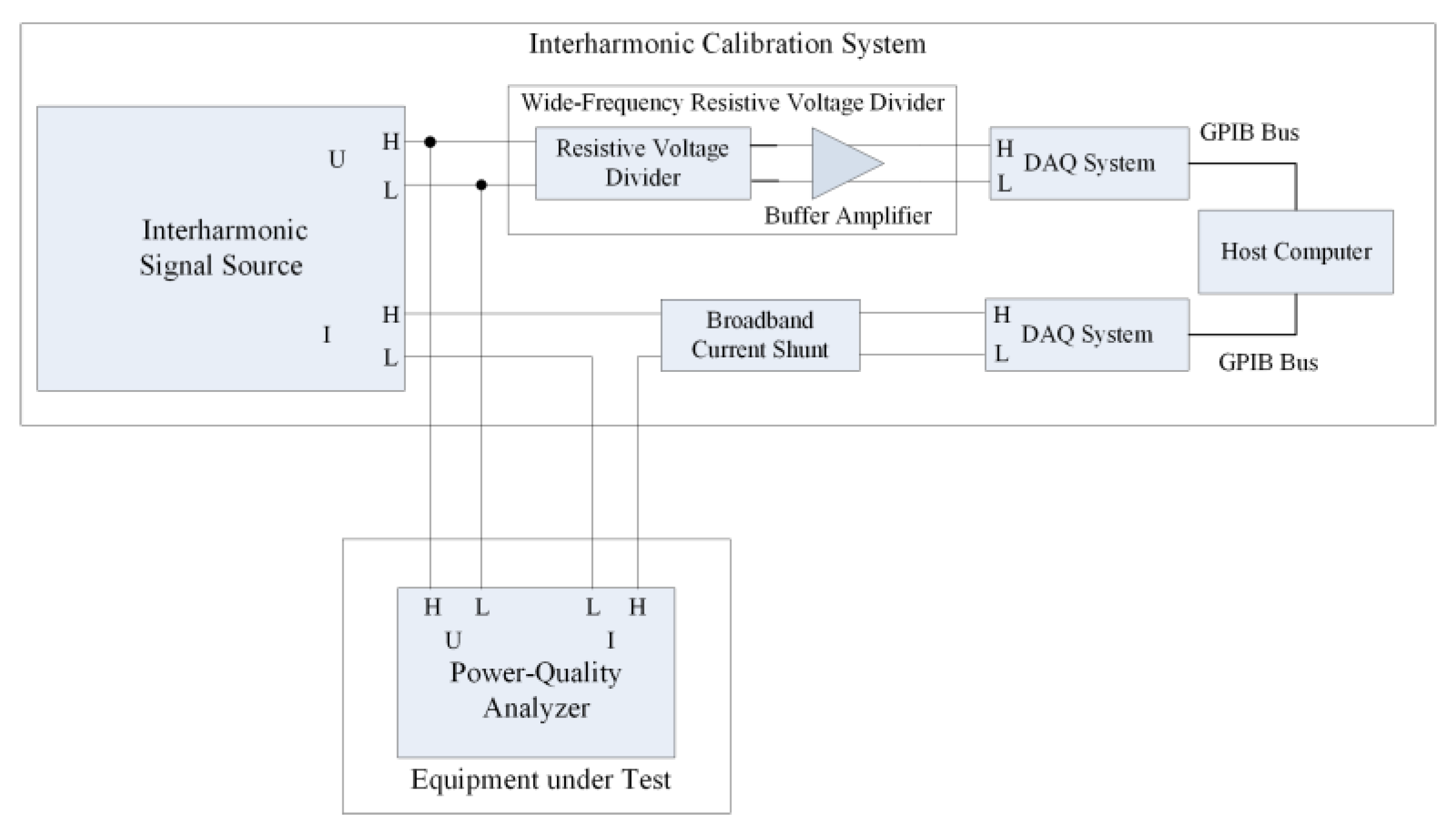
As shown in Figure 1, in our scheme, the interharmonic calibration system mainly consists of an interharmonic signal source, a wide-frequency resistive voltage divider (a combination of a divider and a buffer amplifier), a broadband current shunt, and a high-speed DAQ system. We describe each part in more detail below.
2.1. Interharmonic Signal Source
As a commercial instrument, the Fluke 6105A (Fluke Corporation, Everett, WA, USA) was used to produce the standard interharmonic voltage and current signals for the calibration. The Fluke 6105A can produce signals with a fundamental frequency between 16 Hz and 850 Hz and interharmonic frequencies between 16 Hz and 9 kHz. The accuracy (error) of the interharmonic’s amplitude for Fluke 6105A was 1% (16 Hz to 6 kHz) and 4% (>6 kHz to 9 kHz) for both voltage and current. Fluke 6105A was actually used to first verify the accuracy of our scheme; then, it could be replaced by interharmonic signal sources that do not necessarily reach a certain accuracy.
2.2. Wide-Frequency Resistive Voltage Divider
The wide-frequency resistive voltage divider consisted of a divider and a buffer amplifier. We designed resistive voltage dividers with three rated ratios (75:1, 150:1, and 300:1). When the alternating current (AC) voltage ranges from 30 V to 240 V, the full-scale output voltage can be limited to 0.8 V using a suitable divider. Figure 2 shows the structure of a divider. Resistances with high precision (0.01%) were used to divide the voltage, and the stray parameters were compensated for by capacitances and shield rings.
When measuring high-frequency signals, the input impedance of the sampling device decreases rapidly. Because directly connecting the resistive voltage divider with the DAQ system causes a large error for the ratio, a buffer amplifier was required. The three-level bootstrap unit gain buffer amplifier, which was proposed by Budovsky at the Conference on Precision Electromagnetic Measurements (CPEM; 2010) [25], was used in our design. It was placed between the resistive voltage divider and the DAQ system to enable impedance matching. Figure 3 shows the circuit for the three-level buffer amplifier with output-current amplification.
To verify the performance of the whole resistive voltage divider from 1 Hz to 10 kHz, we performed three groups of experiments as follows:
- Input voltages 37.5 V, 60 V, and 75 V for 75:1;
- Input voltages 75 V, 120 V, and 150 V for 150:1;
- Input voltages 150 V, 240 V, and 300 V for 300:1.
The relative errors for the rated voltage ratios are shown in Figure 4. For relatively low frequencies (<1 kHz), the compensation effect of the capacitances was not clear and the error increased with the frequency. However, for medium frequencies (1 kHz to 6 kHz), the capacitances could compensate for the stray parameters effectively and the error decreased. In addition, for high frequencies (>6 kHz), the effect from stray parameters exceeded the compensation, and the error increased. The overall relative error was below 0.01% (1 Hz to 6 kHz) and 0.04% (>6 kHz to 10 kHz).
2.3. Broadband Current Shunt
The Fluke A40B series (Fluke Corporation, Everett, WA, USA) [26] could be used as the broadband current shunt to measure current with a rated value from 0.1 mA to 100 A and frequencies ranging from direct current (DC) to 100 kHz (see Figure 1). We used shunts with four ranges (200 mA, 2 A, 10 A, and 20 A). The resistance of the shunt is very accurate and stable, with a low self-heating power coefficient and a tiny additional phase-shift. Therefore, it could be directly used to measure both DC and AC, with accuracies of 20 ppm and 23 ppm, respectively.
2.4. DAQ System
Two sets of Agilent 3458A were employed as digital multimeters to enable accurate sampling of voltage and current channels. The multimeters have three sampling modes: DC voltage (DCV) digitizing, direct sampling, and sub-sampling. In our calibration scheme, we used the DCV digitizing mode. This mode uses the DC measurement channel with a sampling frequency between 6 kHz and 100 kHz, and a sampling time between 500 ns and 1 s. The accuracies for the AC voltage and AC current could reach 100 ppm and 500 ppm, respectively. In addition, the accuracy of the frequency was 0.01%, and the time jitter was below 100 ps. During testing, the sampling frequency was set to 40 kHz, and the sample number was 5120. The sampled data from multimeters were transmitted to the computer and analyzed using the LabVIEW software.
2.5. Measurement of the Interharmonic
When calibrating the interharmonics of the power-quality analyzer, the signal generally contains both a fundamental component and the other interharmonic component. If the DAQ system can sample the signal synchronously, i.e., the sampling frequency is an integer multiple of the frequency of each component in the signal, we can obtain the amplitude and phase of the signal with minimal error. However, in most cases, the fundamental frequency and its interharmonic frequencies are unknown. Then, it is difficult to control the DAQ system and implement synchronous sampling. Using asynchronous sampling, the direct application of DFT leads to spectral leakage and the picket-fence effect. As a result, a significant error occurs. The existing methods based on fast Fourier transform (FFT), recommended by IEC 61000-4-7 and Institute of Electrical and Electronics Engineers (IEEE) 1459-2010 standards, can acquire accurate interharmonic parameters only if the signal is sampled synchronously. Under the asynchronous sampling condition, the errors are uncontrolled. In this paper, we propose a new interpolation algorithm to eliminate the error.
The signal is supposed to be sampled by the DAQ system with a sampling frequency fs and a sample number N; and it has the form shown in Equation (1).
where A1, f1, and are the amplitude, frequency, and phase of the fundamental component; A2, f2, and are the parameters of the interharmonic component, supposing (convenient for discussion); and fs satisfies Shannon Theory (fs > 2 max{f1, f2}). is defined as the spectral resolution, and we define parameters and to distinguish the sampling modes. When the signal is synchronously sampled, r1 and r2 are both integers. If the signal is asynchronously sampled, at least one of r1 and r2 is not an integer.
For synchronous-sample mode, the interharmonic’s parameters can be directly calculated by DFT. For asynchronous-sample mode, it can be divided into two cases: only one of the two frequency components is asynchronously sampled, or both of the components are asynchronously sampled. To improve the calibration accuracy under the condition of asynchronous sampling, we propose a new algorithm based on DFT and interpolation. The sampled data are processed using DFT first, and then the interpolation algorithm is applied to eliminate the errors caused by spectral leakage and the picket-fence effects.
For the case that neither of the two components is synchronously sampled, two lines with peak amplitudes in the DFT spectrogram are firstly searched, which are assumed to be the l1-th and the l2-th spectral lines. Secondly, near the l1-th line, another spectral line with its amplitude next to the l1-th line is found, and it is set as the l3-th line. Similarly, the fourth line is found near the l2-th line, and set as the l4-th line. As a result, a total of four lines in the spectrogram are obtained, with their values described as , where and represent the real part and the imaginary part of . Thirdly, we utilize to establish Equation (2). On its left-hand side, the imaginary parts are known. On the right-hand side, is known, while qs (s = 1, 2) and (s = 1, 2) are unknown and can be obtained from Equation (2).
Fourthly, we use to establish Equation (3). On its left-hand side, is known. On the right-hand side, only ps (s = 1, 2) is unknown and can be obtained by solving two equations in Equation (3).
Finally, we acquire the amplitude for each component as follows:
For the case that only one of the two components is asynchronously sampled, it is due to the sampling condition in IEC-approach being able to warrant for the synchronous sampling of fundamental component 50 Hz/60 Hz, but being unable to do so for the interharmonic component. We search two lines with peak amplitudes in the DFT spectrogram, which are assumed to be the l1-th (synchronously sampled component) and the l2-th (synchronously sampled component) spectral line. The frequency of the synchronously sampled component can be directly obtained by f1 = l1 fs/N. Similar to the interpolation approach proposed above, near the l2-th line, another spectral line with its amplitude next to the l2-th line is found, and set as the l3-th line. A total of three lines in the spectrogram are expressed as , and is used to establish equations as shown in Equation (5). On its left-hand side, the imaginary parts are known. On the right-hand side, is known, is known, while qs (s = 1, 2) and are unknown and can be solved by Equation (5).
is used to establish equations as shown in Equation (6). On its left-hand side, is known. On the right-hand side, only ps (s = 1, 2) is unknown and can be solved by Equation (6).
Finally, we acquire the amplitude for each component as follows:
The proposed algorithm above is implemented by software LabVIEW in the host computer of the calibrating system.
3. Results and Discussion
3.1. Error Analysis
Figure 5 shows the hardware implementation of our interharmonic calibration scheme when calibrating the interharmonic voltage. When the wide-frequency resistive voltage divider is replaced by a broadband current shunt, it can be used to calibrate the interharmonic current. The program in LabVIEW has two functions, one is to control the two Agilent 3458A through a general purpose interface bus (GPIB) and, thus, determines the sampling frequency (30 kHz to 40 kHz) and sample number (5120) of DAQ system; the other is to implement the data-processing algorithm. To compare the measurement accuracy of the new algorithm and the IEC-approach, we programed both of them into LabVIEW.
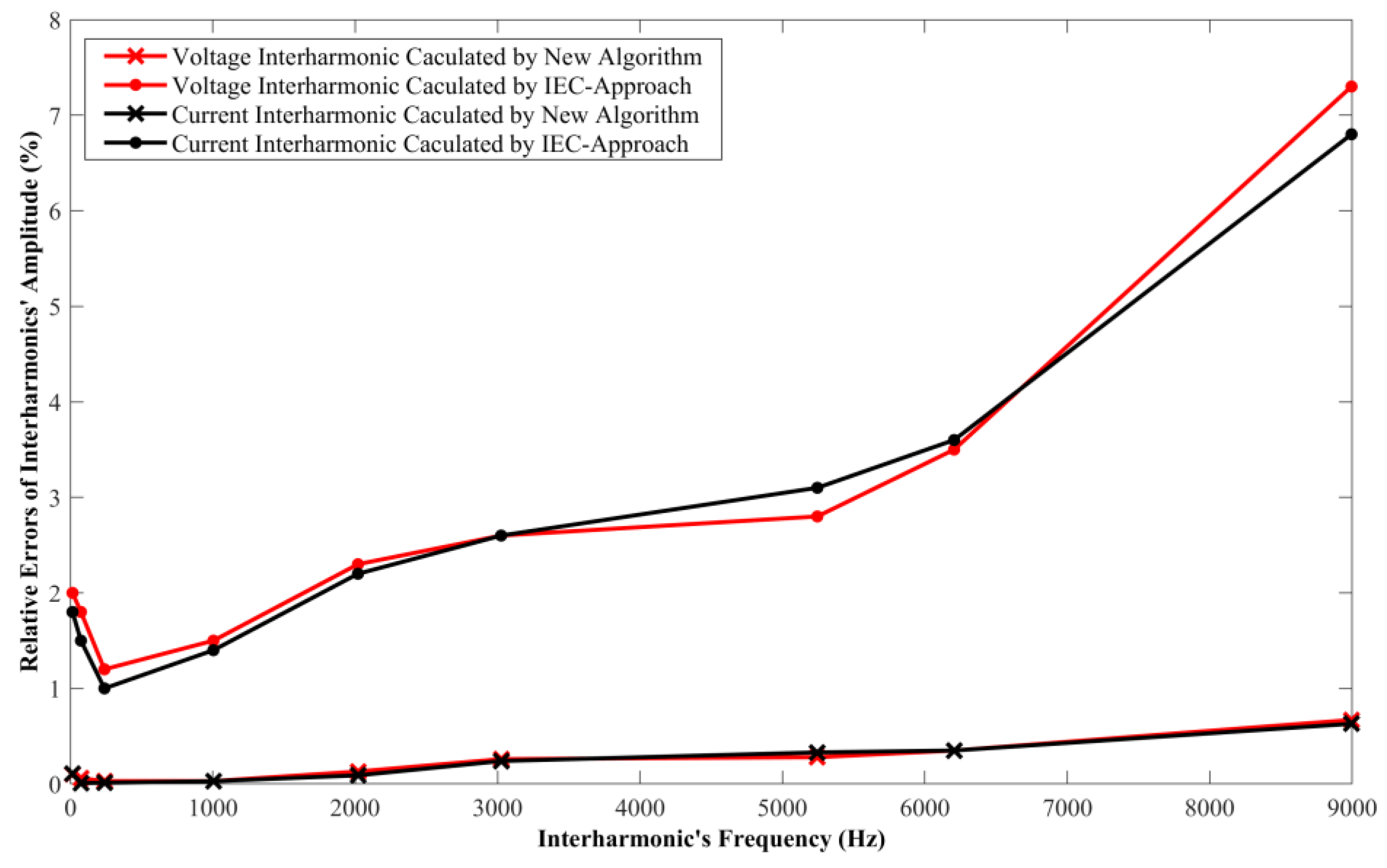
Fifty-eight trials were run, and Figure 6 shows the relative errors of the interharmonics’ amplitude for voltages and currents at different interharmonic frequencies with the range from 16 Hz to 9 kHz. The tests include the measurement of interharmonic voltage and current signals. We set the fundamental frequency as 50 Hz (working frequency in China). The fundamental voltage and current amplitudes were set as 30 V and 1 A, and the interharmonics’ amplitudes were 10% of the fundamental amplitude. The interharmonics’ frequencies were selected according to the IEC standard [27]. Using the algorithm proposed in this paper, we obtained the maximum error of interharmonic amplitudes: for voltage signal, 3.0‰ for 16 Hz to 6 kHz, and 6.8‰ for 6 kHz to 9 kHz; for current signal, 3.5‰ for 16 Hz to 6 kHz, and 6.5‰ for 6 kHz to 9 kHz. However, when the IEC-approach was applied in the system, the maximum errors increased by up to 10 times either for voltage or for current, which indicates that the measurement accuracy of our scheme is higher than that required by the IEC standard.
3.2. Evaluation of the Uncertainty
The interharmonic voltage was measured using a resistive voltage divider and sampled by a DAQ system. The model of the input voltage for the divider is described by Equation (8).
where Uin is the amplitude of the voltage that is delivered to the divider, Uout is the output voltage of the divider and the input voltage of the DAQ, KV is the rated ratio of the divider, and is the error of the ratio. Five sources of uncertainty were considered (see Table 1). We combined them to obtain the standard uncertainty. For the voltage range (30 V to 240 V), the coverage factor was assumed to be two, and the expanded uncertainty was 0.5% (from 16 Hz to 6 kHz) and 2.0% (>6 kHz to 9 kHz), when calibrating the interharmonic voltage.
The interharmonic current was sampled using a current shunt and DAQ system, and the model of the input current for the current shunt can be described by Equation (9).
where Iin is the amplitude of the current delivered to the shunt, Uout is the output voltage of the shunt and the input voltage of the DAQ, KI is the rated ratio of the shunt, and is the error of the ratio. Similar to the voltage calibration, five sources of uncertainty are listed in Table 1. We let the coverage factor be two and obtained the expanded uncertainty 0.3% (16 Hz to 6 kHz) and 1.2% (>6 kHz to 9 kHz) for this current range (100 mA to 10 A).
4. Conclusions
We introduced and investigated an interharmonic calibration scheme for power-quality analyzers in power systems. In the hardware structure of the scheme, we used a Fluke 6105A as the standard interharmonic signal source, a set of Agilent 3458A as the high-speed data acquisition (DAQ) system, and Fluke A40B as broadband current shunt. We also developed wide-frequency resistive dividers (combination of a divider and buffer amplifier). After the signal was fed into the computer, a new algorithm based on both DFT and interpolation was used to analyze the signal under asynchronous sampling. Our results indicate that it can effectively reduce the error for asynchronous sampling.
For the calibration of the interharmonic voltage amplitudes, the interharmonic frequencies ranged from 16 Hz to 9 kHz, the error of amplitude was below 3‰ (16 Hz to 6 kHz) and 7‰ (>6 kHz to 9 kHz), and the expanded uncertainty was 0.5% (from 16 Hz to 6 kHz) and 2.0% (>6 kHz to 9 kHz). For the calibration of the interharmonic current, the interharmonic frequencies ranged from 16 Hz to 9 kHz, the error for the amplitude was below 4‰ (16 Hz to 6 kHz) and 7‰ (>6 kHz to 9 kHz), and the expanded uncertainties were 0.3% (16 Hz to 6 kHz) and 1.2% (>6 kHz to 9 kHz). The accuracy was improved using a thoroughly designed hardware and a new measurement algorithm that is different from the one described in the IEC standard.
Author Contributions
Conceptualization, J.W. and Q.G.; methodology, Q.G. and J.W.; software, Q.G., H.J. and C.P.; validation and data curation, Q.G., C.P., and H.J.; formal analysis, investigation, resources, writing—original draft preparation and writing—review and editing, Q.G. and J.W.; supervision, project administration, and funding acquisition, J.W.
Funding
This research was funded by the National Natural Science Foundation of China, grant number 51777006.
Conflicts of Interest
The authors declare no conflict of interest.
References
- Electromagnetic Compatibility (EMC)—Part 2-1: Environment—Description of the Environment—Electromagnetic Environment for Low-Frequency Conducted Disturbances and Signalling in Public Power Supply Systems, IEC Std. 61000-2-1; International Electrotechnical Commission: Geneva, Switzerland, 1990.
- Electromagnetic compatibility (EMC)—Part 2-2: Environment—Compatibility Levels for Low-Frequency Conducted Disturbances and Signalling in Public Low-Voltage Power Supply Systems, IEC Std. 61000-2-2, 2nd ed.; International Electrotechnical Commission: Geneva, Switzerland, 2000.
- Guillen-Garcia, E.; Zorita-Lamadrid, A.L.; Duque-Perez, O.; Morales-Velazquez, L.; Osornio-Rios, R.A.; Romero-Troncoso, R.J. Power Consumption Analysis of Electrical Installations at Healthcare Facility. Energies 2017, 10, 64. [Google Scholar] [CrossRef]
- Feola, L.; Langella, R.; Testa, A. On the Effects of Unbalances, Harmonics and Interharmonics on PLL Systems. IEEE Trans. Instrum. Meas. 2013, 62, 2399–2409. [Google Scholar] [CrossRef]
- Chen, B.; Pin, G.; Ng, W.M.; Li, P.; Parisini, T.; Hui, S.Y.R. Online Detection of fundamental and interharmonics in AC mains for parallel operation of multiple grid-connected power converters. IEEE Trans. Power Electron. 2018, 33, 9318–9330. [Google Scholar] [CrossRef]
- Voglitsis, D.; Valsamas, F.; Rigogiannis, N.; Papanikolaou, N. On the Injection of Sub/Inter-Harmonic Current Components for Active Anti-Islanding Purposes. Energies 2018, 11, 2183. [Google Scholar] [CrossRef]
- Jain, S.K.; Singh, S.N. Exact Model Order ESPRIT Technique for Harmonics and Interharmonics Estimation. IEEE Trans. Instrum. Meas. 2012, 61, 1915–1923. [Google Scholar] [CrossRef]
- Ramirez, A. The Modified Harmonic Domain: Interharmonics. IEEE Trans. Power Deliv. 2011, 26, 235–241. [Google Scholar] [CrossRef]
- Cataliotti, A.; Cosentino, V.; Cara, D.D.; Tinè, G. LV Measurement Device Placement for Load Flow Analysis in MV Smart Grids. IEEE Trans. Instrum. Meas. 2016, 65, 999–1006. [Google Scholar] [CrossRef]
- Carbone, R.; Menniti, D.; Morrison, R.E.; Testa, A. Harmonic and Interharmonic Distortion Modeling in Multiconverter Systems. IEEE Trans. Power Deliv. 1995, 10, 1685–1692. [Google Scholar] [CrossRef]
- Danzmann, K.; Günther, M.; Fischer, J.; Kock, M.; Kühne, M. High Current Hollow Cathode as a Radiometric Transfer Standard Source for the Extreme Vacuum Ultraviolet. Appl. Opt. 1988, 27, 4947–4951. [Google Scholar] [CrossRef] [PubMed]
- Dupuy, P.; Herman, F. Master Meter Method. In Proceedings of the North Sea Flow Measurement Workshop 1997, Kristiansand, Norway, 27–30 October 1997. [Google Scholar]
- Electromagnetic Compatibility (EMC)—Part 4-7: Testing and Measurement Techniques General Guide on Harmonics and Interhar-Monics Measurements and Instrumentation, for Power Supply Systems and Equipment Connected Thereto, IEC Standard 61000-4-7; International Electrotechnical Commission: Geneva, Switzerland, 2009.
- Lapuh, R.; Voljč, B.; Kokalj, M.; Pinter, B.; Svetik, Z.; Lindič, M. High-Accuracy Measurement of Power Quality Parameters Using Asynchronous Sampling Technique. In Proceedings of the Conference on Precision Electromagnetic Measurements (CPEM), Rio de Janeiro, Brazil, 24–29 August 2014. [Google Scholar]
- Zhou, Z.; Lin, R.; Wang, L.; Wang, Y.; Li, H. Research on Discrete Fourier Transform-Based Phasor Measurement Algorithm for Distribution Network under High Frequency Sampling. Energies 2018, 11, 2203. [Google Scholar] [CrossRef]
- Wu, J.; Zhao, W. A Simple Interpolation Algorithm for Measuring Multi-Frequency Signal Based on DFT. Measurement 2009, 42, 322–327. [Google Scholar] [CrossRef]
- Hui, J.; Yang, H.; Xu, W.; Liu, Y. A Method to Improve the Interharmonic Grouping Scheme Adopted by IEC Standard 61000-4-7. IEEE Trans. Power Deliv. 2012, 27, 971–979. [Google Scholar] [CrossRef]
- Moon, J.-H.; Kang, S.-H.; Ryu, D.-H.; Chang, J.-L.; Nam, S.-R. A Two-Stage Algorithm to Estimate the Fundamental Frequency of Asynchronously Sampled Signals in Power Systems. Energies 2015, 8, 9282–9295. [Google Scholar] [CrossRef] [Green Version]
- Grandke, T. Interpolation Algorithms for Discrete Fourier Transforms of Weighted Signals. IEEE Trans. Instrum. Meas. 1983, 32, 350–355. [Google Scholar] [CrossRef]
- Barros, J.; Diego, R.I. On the use of the Hanning window for harmonic analysis in the standard framework. IEEE Trans. Power Deliv. 2006, 21, 538–539. [Google Scholar] [CrossRef]
- Sala, J.; Durney, H. Coarse time delay estimation for pre-correction of high power amplifiers in OFDM communications. In Proceedings of the IEEE 56th Vehicular Technology Conference, Vancouver, BC, Canada, 24–28 September 2002. [Google Scholar]
- Zhan, Y.; Cheng, H. A Robust Support Vector Algorithm for Harmonic and Interharmonic Analysis of Electric Power System. Electr. Power Syst. Res. 2005, 73, 393–400. [Google Scholar] [CrossRef]
- Miao, J.; Xie, D.; Gu, C.; Wang, X. Correlation Analysis between Wind Speed/Voltage Clusters and Oscillation Modes of Doubly-Fed Induction Generators. Energies 2018, 11, 2370. [Google Scholar] [CrossRef]
- Ahmadipour, M.; Hizam, H.; Lutfi Othman, M.; Amran Mohd Radzi, M. An Anti-Islanding Protection Technique Using a Wavelet Packet Transform and a Probabilistic Neural Network. Energies 2018, 11, 2701. [Google Scholar] [CrossRef]
- Budovsky, I.; Hagen, T. A Precision Buffer Amplifier for Low-Frequency Metrology Applications. In Proceedings of the Conference on Precision Electromagnetic Measurements (CPEM), Daejeon, Korea, 13–18 June 2010. [Google Scholar]
- A40B Precision AC Current Shunt Set Instruction Manual, Fluke. Available online: http://www.fluke.com (accessed on 29 December 2018).
- Hurst, M.; Mittra, R. Scattering Center Analysis via Prony’s Method. IEEE Trans. Antennas Propag. 1987, 35, 986–988. [Google Scholar] [CrossRef]
Figure 1.
Diagram of the interharmonic calibration system.

Figure 2.
Structure of the resistive voltage divider compensated for by capacitances and shielding rings.
Figure 2.
Structure of the resistive voltage divider compensated for by capacitances and shielding rings.

Figure 3.
Circuit schematic for the three-level buffer amplifier with output-current amplification. (Operational amplifier: U1, U2, U3, and U4; Resistance: R_in, R1_1, R1_2, R2, R_load).
Figure 3.
Circuit schematic for the three-level buffer amplifier with output-current amplification. (Operational amplifier: U1, U2, U3, and U4; Resistance: R_in, R1_1, R1_2, R2, R_load).

Figure 4.
Relative errors of rated voltage ratios (75:1, 150:1, and 300:1).

Figure 5.
Hardware implementation for the interharmonic calibration scheme.

Figure 6.
Test results of voltage and current interharmonics’ amplitude.


Table 1.
Uncertainty sources and their calculated values. DAQ—data acquisition.
| Uncertainty Sources | Uncertainty | |
|---|---|---|
| Interharmonic Voltage Measurement | Interharmonic Current Measurement | |
| The instability of the interharmonic source | 0.23% | 0.1% |
| The inaccuracy of the rated ratio of divider | 0.03% | - |
| The inaccuracy of the rated ratio of the shunt | - | 0.002% |
| The inaccuracy of the DAQ system | 0.00023% | 0.00023% |
| The inaccuracy of the measurement algorithm | 0.01% | 0.01% |
| The repeatability of the calibration system | 0.12% | 0.12% |
© 2018 by the authors. Licensee MDPI, Basel, Switzerland. This article is an open access article distributed under the terms and conditions of the Creative Commons Attribution (CC BY) license (http://creativecommons.org/licenses/by/4.0/).
Share and Cite
MDPI and ACS Style
Guo, Q.; Wu, J.; Jin, H.; Peng, C. An Innovative Calibration Scheme for Interharmonic Analyzers in Power Systems under Asynchronous Sampling. Energies 2019, 12, 121. https://doi.org/10.3390/en12010121
AMA Style
Guo Q, Wu J, Jin H, Peng C. An Innovative Calibration Scheme for Interharmonic Analyzers in Power Systems under Asynchronous Sampling. Energies. 2019; 12(1):121. https://doi.org/10.3390/en12010121
Chicago/Turabian StyleGuo, Qiang, Jing Wu, Haibin Jin, and Cheng Peng. 2019. "An Innovative Calibration Scheme for Interharmonic Analyzers in Power Systems under Asynchronous Sampling" Energies 12, no. 1: 121. https://doi.org/10.3390/en12010121
Note that from the first issue of 2016, this journal uses article numbers instead of page numbers. See further details here.