1. Introduction
Historically, electricity power systems have been designed by following a vertical integration scheme: large power generators supply energy to multiple consumers through a hierarchical transport and distribution network. Nowadays, Distributed Energy Resources (DERs) are changing this situation. They consist of a wide range of local generators and storage systems, which are geographically dispersed, generally close to consumption centers and locally managed [
1]. They bring a new conception of electric power systems, with the local user becoming not only a consumer, but also a generator.
Distributed Generation (DG) is a generation structure where small generators are spread over the grid, usually on the consumer side. Distributed Generation (DG) has been growing over the last two decades, arousing a major interest among electric power system planners and operators, energy policy makers and regulators, as well as developers and consumers [
2].
On the other hand, the management of the consumption on electrical grids is receiving increasing attention by research and industry with Demand-Side Management (DSM) [
3,
4]. One of the main objectives of DSM is to smooth the aggregated consumption by reducing the difference between the maximum and minimum consumption power [
5]. This smoothing requires the coordination of thousands or even millions of elements spread over a certain area. The coordination of these elements, to properly use the available resource, becomes a complex task, which is addressed by the smart grids and must be tackled from the multi-agent and distributed system point of view [
6,
7,
8,
9].
Therefore, DSM in smart grids enhances its capabilities regarding the classical electrical grids. The convergence of information and communications technologies (ICTs) with power system engineering allows new levels of automation. DSM in this context is usually formulated as optimization problems, which may be solved by various approaches [
10,
11,
12,
13,
14,
15,
16,
17]. These approaches are also moving towards a new paradigm where the consumer is the center of the grid and goes from being a passive element that only consumes to an active element involved in the management [
18].
The interaction between agents is a key factor in this coordination, which can become highly complex depending on both internal and external factors and is affected by different elements of the environment. Previous works have studied multi-agent coordination with the presence of noise or disturbances [
19]. However, the environment may affect the coordination process, not only as noise or disturbance, but the nature of the coordination process itself. In such a case, the coordination between agents may be considered as an adaptive process to the environment where they are. This adaptive process may be designed so that the environment meets certain predefined characteristics or goals.
In this paper, the environment is an electrical grid, and SwarmGrid focuses on the problem of smoothing the aggregated consumption in an environment where Distributed Generation (DG) is part of the system. SwarmGrid takes advantage of one main feature of the consumption in the electrical grids: its periodicity. The consumption profile almost repeats every day, week or season. SwarmGrid focuses on the coordination of distributed multi-agent systems from the frequency domain perspective, based on previous works on multifrequency coupled oscillators [
20]. This work develops an algorithm that is able to coordinate an n-elements system by using the periodicity of the environment.
The remainder of this paper is as follows. The environment approach and the definition of the multi-agent electrical system are presented in
Section 2. The SwarmGrid algorithm is defined in
Section 3.
Section 4 describes the simulated environment and its generation and consumption parameters. In
Section 5, experiments with different penetrations of Distributed Generation (DG) are evaluated. A discussion is presented in
Section 6, and the paper is concluded in
Section 7.
2. Environment Definition
2.1. Facility
A facility is defined as an electric power system that belongs to a particular consumer. In this paper, it may be composed of two types of elements: generation and consumption. The proposed algorithm will control the consumption in order to modify the power flow between facilities and the grid.
Consumption
Consumption is the most heterogeneous part of an electrical power system. There is a huge variety of devices that consume electricity with different characteristics: nominal power (from an LED lamp to industrial ovens), intermittent consumption (e.g., a fridge pump that activates periodically), peak power (e.g., the use of a drill), etc. For the implementation of Demand-Side Management (DSM) techniques and the deployment of the SwarmGrid algorithm, it is particularly interesting to classify the consumption by means of its controllability. In this way, consumption can be divided into fixed, deferrable and elastic types [
21]. The electric vehicle can be also included as elastic consumption that can be positive when it is charging or negative when it is discharging. In this aspect, the SwarmGrid algorithm could be also used for electric vehicle fleet charging management [
22].
2.2. Environment
In this paper, the electrical grid is defined as a single node disregarding losses and transmission delays. The electrical grid contains facilities of different users, which contain in turn different electrical loads. The consumption in time of the facility i is represented as the power signal . The sum of all facilities in the electrical grid is the aggregated consumption such that , where M is the number of facilities in the electrical grid.
Each facility is divided into a controllable and a non-controllable part. The non-controllable () part represents all consumptions that cannot be managed, that is a fixed consumption. The controllable part () represents consumption that can be managed, deferrable or elastic.
Therefore, the aggregated consumption
of the complete electrical system is defined as the total energy consumed by all facilities, which can be decomposed into a sum of controllable or non-controllable signals, so that:
2.3. Metrics
Two different metrics will be used to study the behavior of the network, the self-consumption factor and the crest factor.
2.3.1. Self-Consumption Factor
The self-consumption factor (
) represents the fraction of the electrical energy consumed by the loads, which is only supplied by the local generation sources [
21,
23]:
where
is the energy directly supplied by the Photovoltaic (PV) generator to the loads and
is the total energy consumed by the loads. The range of
is
, because this factor is normalized by the total consumption of the local facility.
2.3.2. Crest Factor
In order to analyze the variability of the aggregated consumption, the crest factor
C has been used. It is a measure of a waveform, showing the ratio of peak values to the average value, such that:
where
N is the number of samples taken from the aggregated consumption,
is the absolute value of the maximum peak and
is the root mean square. The crest factor makes reference to a concrete time interval in which the signals are evaluated together with a concrete sample period. This factor is in the range
, one being the optimal value where the aggregated consumption is completely flat. In this paper, the time interval is denoted with a subscript, for example
,
,
and
.
3. SwarmGrid
Two specific objectives can be tackled when trying to schedule loads in the electric system: to maximize the use of local generation or to maximize the aggregated consumption smoothing. The first one is a local objective, taking into account local generation and consumption without the need for any information or interest in the environment. This objective maximizes the self-consumption factor. On the other hand, the second objective is a global objective, which takes into account the aggregated consumption to reduce the difference between peaks and valleys, being related with the crest factor.
Unfortunately, both objectives can be very antagonistic. The proposed SwarmGrid algorithm is designed to meet a compromise between both objectives by scheduling deferrable loads in every facility of the system. Therefore, SwarmGrid schedules loads in local facilities, which affect the global shape of the aggregated consumption by means of a self-organized coordination.
3.1. Modeling
In the SwarmGrid algorithm, the environment is modeled from the signal processing point of view dividing the consumption into its periodic components. In this way, the consumption smoothing problem can be seen as a frequency filtering where the controllable consumption filter is the non-controllable part. When extended to multiple agents in the system, this process is performed in a distributed way. Therefore, the controllable part of every facility can be represented as a sum of sinusoidals, such that:
where
is the amplitude,
the frequency and
the phase of each component of each of the
N signals in which
is decomposed.
For the sake of privacy, facilities do not have a direct communication system, and they can only coordinate by observing the aggregated signal
. Therefore, the shape of
must be controlled in a distributed way such that
and
are modified to smooth the aggregated consumption. This modeling is exhaustively described in [
20]. This approach takes advantage of the periodic behavior of the consumption allowing load schedules without time limit and in a stable way.
3.2. Load Scheduling
In all facilities, users request to activate some loads at specific times. If these loads are fixed, they must be instantaneously activated. However, if they are deferrable or elastic, they may be scheduled in terms of time and amplitude. In the SwarmGrid algorithm, the scheduling consists of the assignment of an activation time
for each deferrable load controlled, where the subscript
i denotes that the deferrable load belongs to facility
i and the subscript
j is an identifier of the deferrable load. When the user requires performing a deferrable load, he/she must indicate which load must be performed together with its running range
. The algorithm is responsible for scheduling the task deciding
, satisfying that this time instant is within the running range. The consumption of these deferrable loads is expressed by the following equation:
As previously mentioned, the scheduling consists of the assignment of
for each incoming deferrable load. This assignment is performed by using a local consumption pattern, denoted by
.This pattern defines the objective shape of the local consumption. It means that the deferrable load should be scheduled such that the local consumption has the same shape as
. In order to achieve this objective, the local consumption pattern is defined as a probability density function
. Therefore, the activation time is considered as a random variable, which takes on a value with a certain probability described by
. The following equation connects
with
:
where
K is a normalizing factor, which is required for
, being a probability density function.
However, the local consumption patterns have two objectives on the SwarmGrid algorithm: to smooth the aggregated consumption and to increase the self-consumption. In order to achieve these objectives,
has been divided into two parts. The first part is a function based on a multi-agent coordination algorithm, Multi-Frequency Coupled Oscillators (MuFCO) [
20]. This function is able to smooth the aggregated consumption regardless of the number of elements that participate. The second part is the Photovoltaic (PV) generation forecast function
. This function is able to increase the self-consumption of the local facility. Both parts are combined in the following equation:
where
is a parameter that regulates the importance of the previous two functions in
. This means that if
, the local consumption pattern tends to
and the scheduling tends to smooth the aggregated consumption. On the other hand, if
, the local consumption pattern tends to
and the scheduling tends to increase the self-consumption.
3.3. Scheduling with MuFCO
If the SwarmGrid algorithm is configured with
, it only uses
to generate the local consumption pattern. The Multi-Frequency Coupled Oscillators (MuFCO) algorithm is in charge of generating consumption patterns to smooth the aggregated consumption where
n individuals participate.
n has no upper theoretical limit, getting a more sinusoidal form of the signal as the number of individuals increases [
20]. This smoothing process is summarized in the reduction of the amplitude of
through the control of amplitudes
and phases
of every facility.
Thus, a facility is considered as an individual oscillator, which is shifted in magnitude, such that:
Therefore, the sum of all facilities has the same properties as the collective of oscillators generated by the Multi-Frequency Coupled Oscillators (MuFCO) algorithm. The facilities observe the aggregated consumption signal and generate sinusoidal functions such that they adapt to the non-controllable consumption and smooth the aggregated consumption.
The sinusoidal function for a local facility
i is directly used as a probability density function when
, such that:
3.4. Scheduling with PV Forecast
In order for the SwarmGrid algorithm to improve the self-consumption of the locally-generated electricity, a local energy generation forecast should be included in the scheduling process [
24]. In this section, the SwarmGrid algorithm is configured with
; thus, it only uses
to generate the local consumption pattern.
is the normalized Photovoltaic (PV) generation forecast for the facility
i. This function is normalized by the maximum generation of the Photovoltaic (PV) generator. This means that
is in the range
. The normalized Photovoltaic (PV) generation forecast for a local facility
i is directly used as a probability density function when
, such that:
3.5. Real-Time Execution
The SwarmGrid algorithm has been designed to run in real-time. It is locally executed when a new deferrable load is required by the user, and this event can occur at any time. Thus, the SwarmGrid algorithm is an asynchronous algorithm. When a new deferrable load is required, this algorithm is executed. The algorithm begins by obtaining the information of the deferrable load to be scheduled. This information comes directly from the user. Once the user has indicated the required information, the SwarmGrid algorithm calculates
from the Multi-Frequency Coupled Oscillators (MuFCO) algorithm. This means that the SwarmGrid algorithm asks for
and
for the Multi-Frequency Coupled Oscillators (MuFCO) algorithm and calculates the sinusoidal function; see Equation (
9).
is also calculated through Equation (
10). The local consumption pattern
is calculated by using Equation (
7). Once
is obtained,
can be calculated in the range
by using Equation (
6). Finally,
is calculated for this deferrable load. The value of
is taken on from
as the execution of a random variable.
4. Simulator Definitions
4.1. GridSim Simulation Framework
All examples of the SG algorithm operation have been performed in the GridSim simulation framework (
https://github.com/Robolabo/gridSim). GridSim is a simulator developed to analyze the power balances on a virtual electrical grid. The grid is composed of lines. A line represents a set of nodes with the same characteristics. The nodes are complex elements connected to the lines, which can be equipped with different types of consumption, DERs and control systems. These nodes can represent a single device to a fully-equipped facility. In addition, a base consumption function can be added to the grid. It represents a non-controllable consumption, which is added to the aggregated consumption of the simulated grid.
All experiments have been done through simulations of an electrical grid divided into 600 nodes. Each node is a facility that is equipped with a Photovoltaic (PV) generator, a storage system and local consumption. The time step of simulation is 1 min. In this analysis, a virtual user is used in order to generate the consumption profile. This user belongs to a concrete facility; this means that if there are 600 nodes, there are 600 virtual users.
4.2. Virtual Users
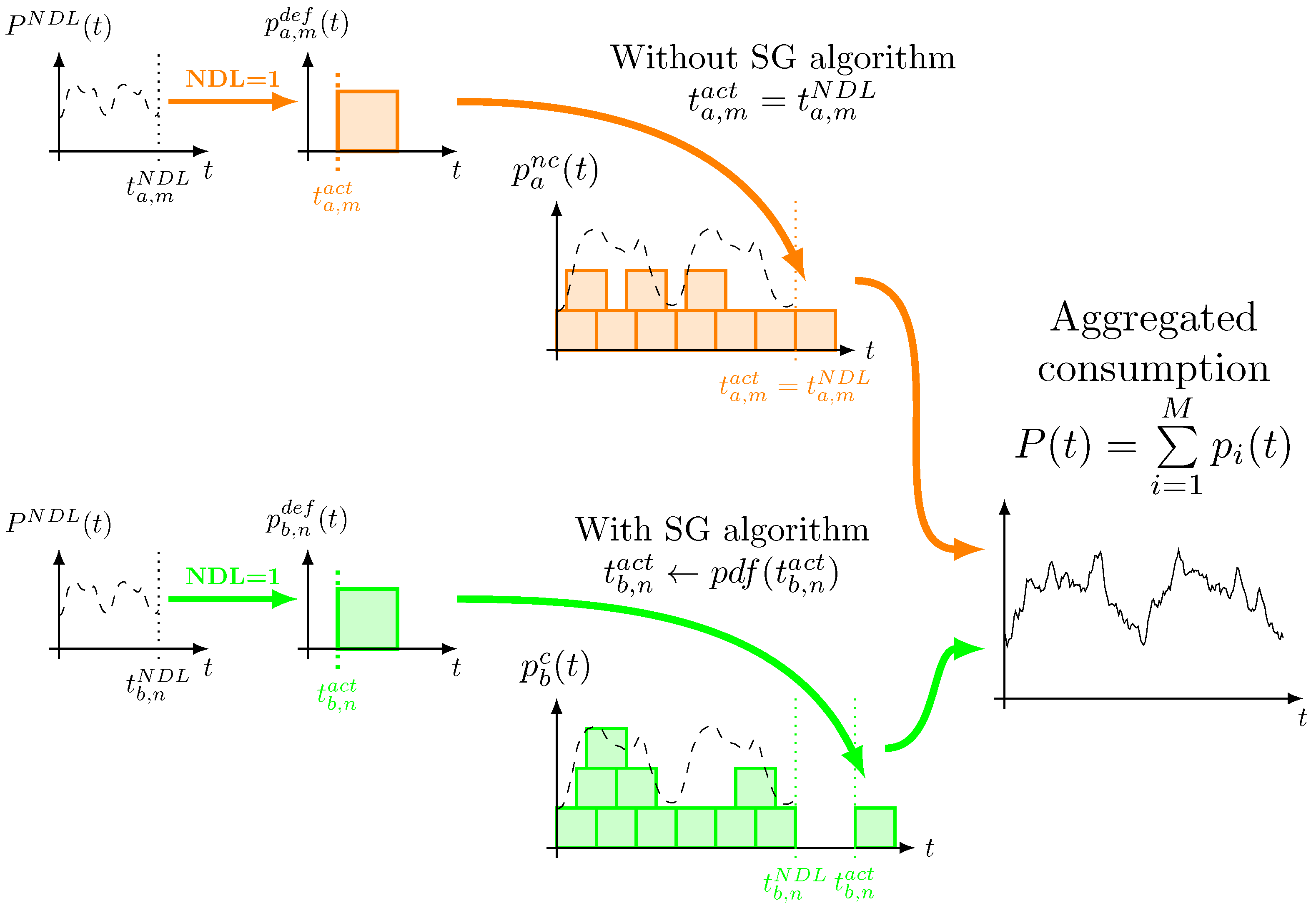
The consumption of the local facilities (nodes) is created by virtual users in the GridSim simulator. In this analysis, the virtual users only create deferrable loads. Thus, the user of each facility requires a number of deferrable loads during the execution of any simulation. This requirement is an asynchronous event, which represents a new deferrable load creation in the local facility. It could happen at any time step of the simulation. Every new deferrable load is created at a concrete time instant denoted by
. If no controller schedules the load, it is activated when it is created such that
.
Figure 1 shows an example of this procedure for two facilities where one facility is equipped with the SwarmGrid algorithm and the other has no controller.
Virtual users create new deferrable loads randomly. There is a probability density function that defines the probability that a new deferrable load is created at a given time instant. This function is denoted by . Thus, the creation of a new deferrable load is a binary random variable . Every time step of the simulation, it is checked if there is a new deferrable load . For the analysis presented in this paper, is the real aggregated consumption of peninsular Spain during 2017. This implies that the consumption of the virtual users has a similar shape as this aggregated consumption. SwarmGrid controllers modify the activation time of the deferrable loads; thus, it is satisfied that .
Moreover, deferrable loads are modeled as energy packets. These packets consume a constant nominal power
P during a certain time interval
; see
Figure 1. To perform the following analysis, the nominal power is
, and duration is
. In addition, it is considered that the deferrable loads have a running range of one day (1440 min):
and
. Each user creates around 12,200 deferrable loads per year. Thus, a local facility consumes around 410 GWh per year. The sum of all local facilities has a yearly energy consumption of around 246 TWh, equal to the Spanish yearly consumption. In a real electrical grid, the facilities do not consume as much electrical energy as the simulated facilities. These energy amounts have been chosen because the grid has been divided into 600 facilities to reduce the computing load. Simulating an electrical grid with thousands or millions of facilities causes a very high computation time. On the other hand, 600 facilities are enough to observe the coordination and smoothing capacity of the SG algorithm.
4.3. Local Generation
Local, specifically PV, generation should be included in the facilities in order to use the local controllers. In the simulated experiment, the Photovoltaic (PV) generation is considered as a negative consumption [
25]. If a facility has a generation excess of 1 kW, it is consuming −1 kW. This consideration allows to introduce the Photovoltaic (PV) generation in the aggregated consumption and observe its effects. As a final aspect to be appreciated, the aggregated consumption is always positive. This means that if the Photovoltaic (PV) generation is greater than the whole consumption of the grid, the aggregated consumption will be zero instead of taking negative values.
The generation profiles from six different cities of Spain have been used: Cáceres, Ciudad Real, Logroño, Madrid, Santiago and Soria. The calculation of the Photovoltaic (PV) generation profiles has been done by using the real irradiance data from these cities during 2017. This irradiance has been translated to AC power by using a model of the Photovoltaic (PV) generators and weather forecasting of an energy self-sufficient solar house located in Madrid [
24]. There are 100 virtual facilities (nodes) deployed in each city. The combination of these cities allows to consider different climate regions. This heterogeneous generation is representative of the national generation.
The maximum nominal Photovoltaic (PV) power generation in each facility is 240 MW, such that the total power generation of all facilities is 144 GW. This generation power corresponds to a yearly energy generation of around 246 TWh, which is the same energy amount as the yearly peninsular energy consumption of Spain.
5. Simulation Experiments
In this section, the SwarmGrid algorithm’s operation is analyzed. This analysis focuses on validating the SwarmGrid algorithm and studying the improvement that it brings to the electrical grid. All analyses presented in this Section are based on the 2017 consumption data of the Spanish grid. This section analyzes two different scenarios:
The grid without DG: in this scenario, there are no Distributed Energy Resources (DERs), and the SwarmGrid algorithm just manages the consumption of the electrical grid to smooth the aggregated consumption. The SwarmGrid algorithm schedules the deferrable loads only by using the sinusoidal patterns generated by Multi-Frequency Coupled Oscillators (MuFCO); thus, for this scenario.
The grid with DG: in this scenario, local Photovoltaic (PV) generators are included in the local facilities as Distributed Generation (DG) without electrical storage.
5.1. The Grid without DG
In this scenario, the facilities are purely consumers without local generation. This is the common scenario if the SwarmGrid algorithm is deployed in buildings without Distributed Energy Resources (DERs) where the classical Demand-Side Management (DSM) mechanisms are performed. Part of this consumption is controlled by the SwarmGrid algorithm, and the other part is directly set by the user. The percentage of consumption controlled by the algorithm is denoted by . For example, if = 50% and the yearly consumption is 246 TWh, this means that the SwarmGrid algorithm controls 123 TWh of deferrable loads along the year. Notice that for all experiments performed in this scenario because there is no local generation.
A campaign of experiments has been performed to study how the percentage of consumption controlled by the SwarmGrid algorithm affects the crest factors of the aggregated consumption. For each value, 100 experiments have been performed with different seeds of the random number generator. An experiment consists of the simulation of the previously explained electrical grid during one year and a half (788,400 min) with a concrete value and a concrete seed. The first half of the year is used to adapt the SwarmGrid algorithm to the grid; after that, the crest factors are calculated for the remainder of the year.
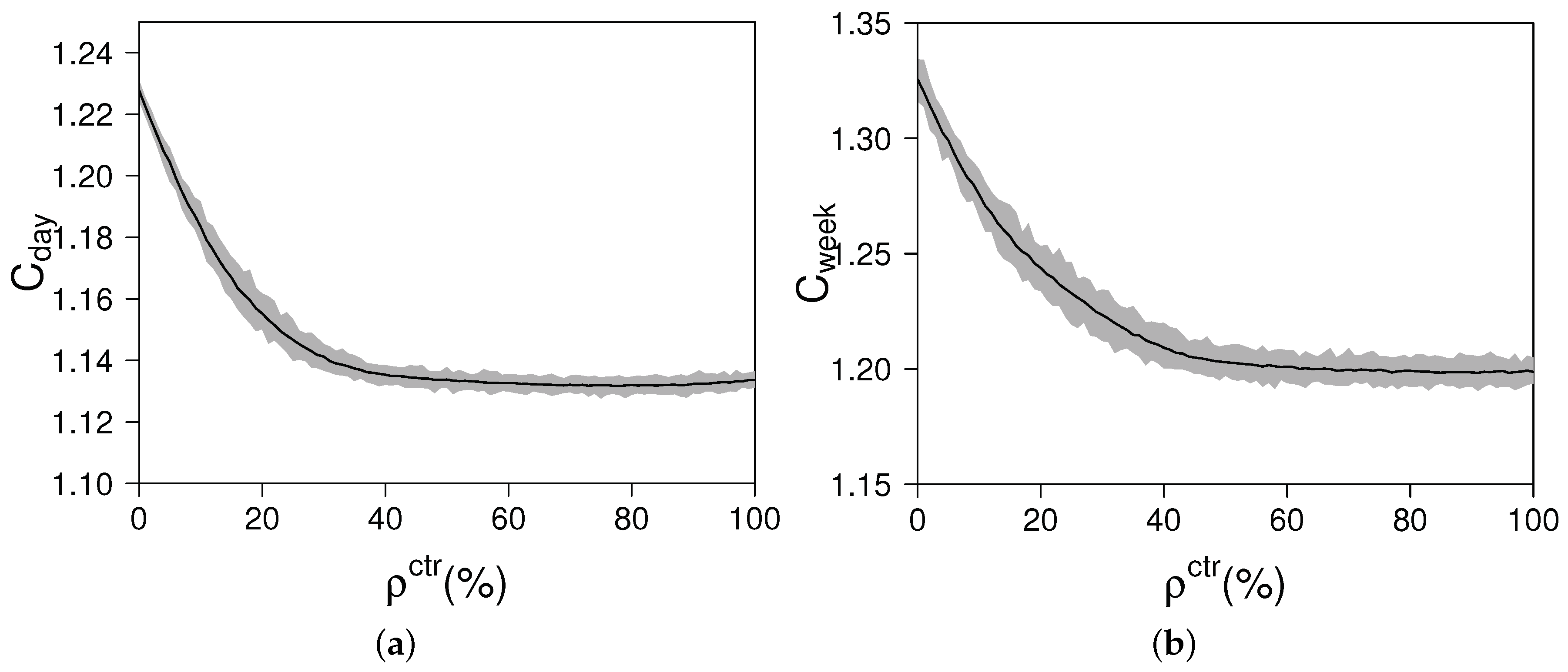
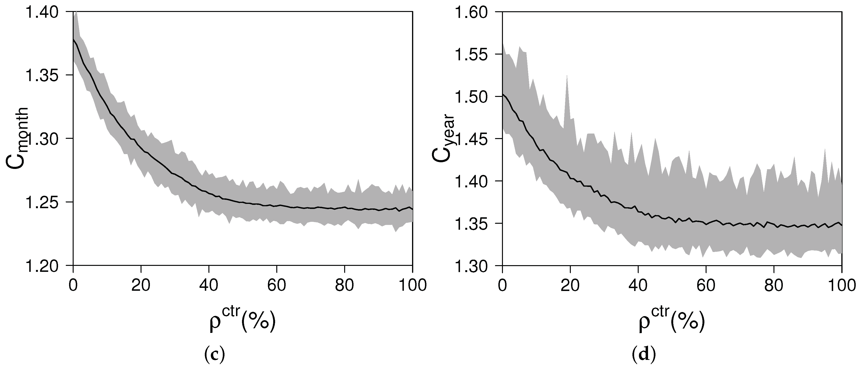
Figure 2 shows the development of the crest factors for different percentages of consumption controlled by the SwarmGrid algorithm. For each
value, the mean and the maximum and minimum values have been calculated from the 100 different seeds.
Figure 2 is divided into four graphs where each graph plots the statistical analysis for each type of crest factor. The common trend is that the greater the amount of consumption controlled by the algorithm, the lower the crest factors are. In addition, the dispersion of the experiments is higher the greater is the range of time covered by the crest factor. For instance, the difference between
and
is much lower for the daily crest factor average than for the yearly crest factor average. In all graphs, the crest factors achieve a plateau value when the SwarmGrid algorithm controls over 50% of the whole consumption. The following conclusions come from these results:
Regardless of , the algorithm reduces the electrical grid variability: in general, the higher , the lower the crest factors. This implies that the smoothing objective is met by the SwarmGrid algorithm. This relationship is satisfied until the crest factors achieve the plateau value. When this value is achieved, the algorithm self-organizes, and the crest factors may not be reduced.
The algorithm self-organizes: For < 50% values, the controllable part of the grid’s consumption is lower than the non-controllable one. The SwarmGrid algorithm adapts to the non-controllable consumption, reducing the variability of the grid. On the other hand, when > 50%, the SwarmGrid algorithm should also self-organize. This means that the controllable consumption must coordinate with itself to achieve a neutral effect. For example, if = 60%, there are 240 facilities without the SwarmGrid algorithm; thus, 240 facilities with the SwarmGrid (SG) algorithm are required at least to fully smooth their consumption. The other 120 facilities with the SwarmGrid algorithm should coordinate among each other to provoke a constant aggregated consumption. This feature is verified because the crest factors do not increase for > 50%. This implies that the controlled consumption is able to coordinate to reduce the crest factors for < 50% values and to maintain them for > 50%.
5.2. The Grid with DG
The presence of Distributed Generation (DG) in the electrical grid may increase the variations in the aggregated consumption. In this scenario, the effects of the Photovoltaic (PV) generation together with the SwarmGrid algorithm are analyzed. The generation profiles from six different cities of Spain have been used. There are 100 virtual facilities (nodes) for each city. The combination of these cities allows different climate regions to be considered. The maximum nominal Photovoltaic (PV) power generation is 240 MWp in each facility, such that the sum of the generation of all facilities is 144 GWp. This generation power corresponds to a yearly energy generation of around 246 TWh, which is the same energy amount as the yearly energy consumption of Spain. In this section, the effects of the Photovoltaic (PV) penetration in the electrical grid have also been studied by using the Photovoltaic (PV) penetration factor .
The SwarmGrid algorithm modifies the aggregated consumption shape and the self-consumption of the local facilities depending on the
parameter when there is Photovoltaic (PV) generation. A campaign of experiments has been performed to study how
and
affect the crest factors of the aggregated consumption and the self-consumption. In this campaign,
= 100% for all experiments so that the effect of the
parameter could be better observed. Different combinations of
and
have been studied. For each combination of these parameters, 30 experiments have been performed with different seeds of the random number generator. An experiment consists of the simulation of the previously explained electrical grid during one year and a half (788,400 min) with a concrete combination of
and
and a concrete seed. The first half of the year is used to adapt the SwarmGrid algorithm to the grid, and after that, the crest factors are calculated for the remainder of the year. The crest factors and the self-consumption of the local facilities are calculated for each experiment. The SwarmGrid algorithm operates with the tuned parameters to reduce the daily variability obtained in [
20]:
,
,
and
.
Figure 3 shows the development of the crest factors for different combinations of
and
with
= 100%. In general, the lower the
parameter is, the lower the electrical grid variability. When
takes values close to one, the variability of the grid increases exponentially. The greater the
parameter is, the greater the importance that is given to the Photovoltaic (PV) generation forecast. Analyzing the effects of the forecast error is not the objective of this paper; for this reason, the ideal forecast model has been used. The Photovoltaic (PV) generation forecast of a day is exactly the generation of that day. In these situations, all facilities schedule the deferrable loads following a similar pattern (the Photovoltaic (PV) forecast) without synchronization. This implies that days with low Photovoltaic (PV) generation or forecast errors cause a great mismatch between consumption and generation. These results suggest that the SwarmGrid algorithm works better for
from the grid point of view.
During the remainder of this section, is zero to focus on the smoothing of the aggregated consumption.
The effect of the percentage of consumption controlled by the SwarmGrid algorithm on the aggregated consumption depends on the Photovoltaic (PV) penetration. A campaign of experiments has been performed to study how and affect the crest factors of the aggregated consumption and the self-consumption. In this campaign, is zero because of the results of the previous analysis. Different combinations of and have been studied. For each combination of these parameters, 30 experiments have been performed with different seeds of the random number generator. An experiment consists of the simulation of the previously explained electrical grid during one year and a half (788,400 min) with a concrete combination of and and a concrete seed. The first half of the year is used to adapt the SwarmGrid algorithm to the grid, and after that, the crest factors are calculated for the remainder of the year. The crest factors and the self-consumption of the local facilities are calculated for each experiment.
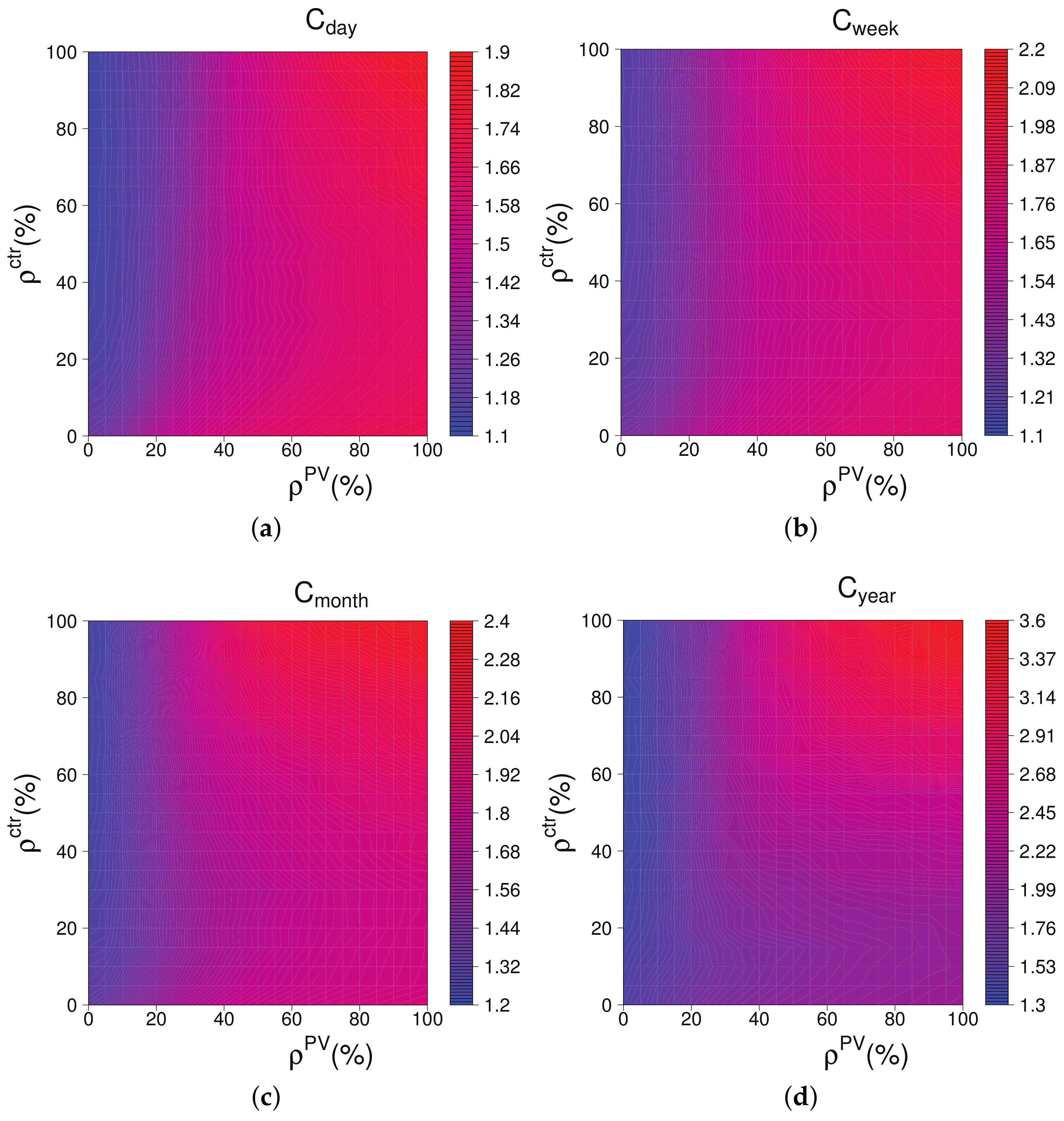
Figure 4 shows the development of the crest factors for different combinations of
and
with
. The effect of the SwarmGrid algorithm on these factors changes depending on the Photovoltaic (PV) penetration. For low values of
, the higher
, the smoother the aggregated consumption. The SwarmGrid algorithm is able to synchronize with the electrical grid and to reduce the crest factors. On the other hand, for high values of
, the increase of
intensifies the variability introduced by the Photovoltaic (PV) generation.
Figure 4 shows the development of the self-consumption for different combinations of
and
with
. As in previous analysis, the self-consumption increases with
because of the Photovoltaic (PV) resource availability. Moreover,
enhances the self-consumption, as well. This implies that the SwarmGrid algorithm synchronizes with the Photovoltaic (PV) generation because it is included in the aggregated consumption signal.
6. Discussion
The SwarmGrid algorithm has a number of valuable features for Demand-Side Management (DSM) that it borrows from swarm intelligence and coupled oscillators algorithms: self-organization, adaptability, low information exchange, local conditions and anonymous communication:
Self-organization: An electrical grid with facilities equipped with the SwarmGrid algorithm is able to self-organize. All facilities schedule the deferrable loads following a common goal. Without an explicit information exchange and without the presence of a central agent, the consumption of these facilities organizes over time. This feature could be observed in
Section 5.1, when the amount of controllable consumption exceeds the amount of non-controllable consumption. This feature differs from centralized and distributed algorithms based on other techniques. The centralized algorithms cannot self-organize by definition, and the loss of the central agent causes a complete operation failure. Other distributed techniques typically perform DSM through a negotiation between agents. These processes requires direct communication between agents, causing operation failures when this communication is lost.
Adaptability: Facilities are able to adapt to the aggregated consumption of the grid. A non-controllable consumption was introduced in the simulated electrical grid. The SwarmGrid algorithm schedules the deferrable loads adapting to the non-controllable consumption and smoothing the aggregated consumption. All DSM algorithms require certain adaptability; however, the main difference of SwarmGrid in relation to other techniques is that this adaptability is performed for each agent by dividing this feature into thousands or millions of elements. This feature is also implemented by other distributed algorithms, being an advantage in comparison with centralized approaches.
Low information exchange: The SwarmGrid algorithm requires a very low information exchange. The facilities only require the aggregated consumption signal, which should be provided by the electrical grid operator. In addition, the sample period of this signal implies a low computing load compared to the current electronics: in the examples shown. Swarm intelligence-based algorithms are based on relative simple calculations for each agent, but they achieve complex behaviors when working as a swarm. This feature is acquired by SwarmGrid , which implies lower computing requirements in relation to other DSM algorithms.
Local conditions: The SwarmGrid algorithm takes into account local conditions. It schedules the deferrable loads by considering the grid and the local Photovoltaic (PV) generation forecast. In addition, this algorithm could be designed to satisfy other local conditions because its distributed in nature. This feature is a general advantage of the distributed approaches regards the centralized ones. Each agent participates in the DSM process, but at the same time, it can improve its local performance.
Anonymous communication: The SwarmGrid algorithm does not require communicating the local state to other elements of the grid. This is an advantage in comparison with other centralized and distributed algorithms. In centralized algorithms, the local state must be communicated to the central agent. Moreover, other distributed approaches typically require information exchange between agents. SwarmGrid ensures that local information is not transmitted, keeping the system as simple as possible and improving the security of the user.
The smoothing of the aggregated consumption by the SwarmGrid algorithm could be observed in different scenarios in
Section 5. In general, the SwarmGrid algorithm reduces the crest factors of the electrical grid proportionally to the amount of controlled energy. This issue is easily observed in the analysis of the SwarmGrid operation without DG technologies. In this case, the SwarmGrid algorithm schedules a certain percentage of energy of the electrical grid. The results conclude that for an amount of energy controlled by the SwarmGrid algorithm lower than 50%, the higher the percentage of controlled energy, the lower the crest factors. For percentages higher than 50%, the crest factors achieve a plateau value. This is because the SwarmGrid algorithm adapts to the non-controllable consumption and schedules the remaining controllable consumption so that the variability of the aggregated consumption does not increase. This is indicative of the self-organization capacity of the algorithm. Two examples have been proposed to show how the SwarmGrid algorithm affects the shape of the aggregated consumption and its difference between peaks and valleys. Thanks to the use of the algorithm, the maximum yearly peak has been reduced from 41.9 GW to 36.1 GW, maintaining the same average consumption. This implies that the size of the electrical grid has been improved because the average consumption is closer to the minimum peak: less electrical infrastructure is required, which is used more often on average. In addition, the average daily difference between peaks and valleys has been reduced from 12.2 GW to 4.7 GW. This implies that the daily use of the electrical grid has also been improved: the difference between peaks and valleys is much lower, and thus, the grid does not have to respond to such abrupt power variations, increasing its stability.
Generally, the presence of large amounts of Photovoltaic (PV) generation makes the smoothing process of the aggregated consumption difficult. The cause of this malfunction is typically the same: all facilities schedule the deferrable loads to run during the same time period without considering other facilities. This causes a consumption peak at this period, which may be increased because of a lack of generation or a bad forecast. On the other hand, the local self-consumption is enhanced when . Thus, a compromise between aggregated consumption smoothing and self-consumption should be found. This compromise depends on the specific requirements where the SwarmGrid algorithm is implemented.
7. Conclusions
In this paper, Demand-Side Management (DSM) has been tackled from the electrical grid point of view, but actions are taken on the consumer side. This means that the local consumption is managed to smooth the aggregated consumption of the grid, where every user takes only into account its local conditions. A Demand-Side Management (DSM) algorithm, SwarmGrid, has been developed to address this issue. The proposed algorithm is developed from a distributed point of view; thus, the Demand-Side Management (DSM) is not performed by a central agent, but each consumer is actively involved in its implementation. Direct communication between users or facilities has also been avoided. Thus, the coordination is performed with the sole information of the aggregated consumption of the grid.
The proposed SwarmGrid (SwarmGrid ) algorithm uses the frequency consumption patterns generated by the Multi-Frequency Coupled Oscillators (MuFCO) algorithm and takes into account the local generation. It generates a pattern by combining the aggregated consumption and Photovoltaic (PV) generation forecasts to schedule the deferrable loads. In general, the SwarmGrid algorithm is able to smooth the aggregated consumption in every scenario. The improvement caused by the SwarmGrid algorithm is more relevant for low percentages of controllable power. It achieves a plateau value after the controllable energy of the whole electrical grid reaches 50%. This means that the deferrable power controlled by the SwarmGrid algorithm is able to adapt to the non-controllable power. Thanks to the use of this algorithm, the maximum yearly peak and the daily difference between peaks and valleys are reduced.
Some future developments of the SwarmGrid algorithm are discussed below. The SwarmGrid algorithm has been designed to schedule deferrable loads, but it is not the only type of load. Elastic loads, whose consumption can be controlled directly, could be also included. For example, the power of an electric pump can be modified to shape a sinusoidal pattern. Several loads are a mix between deferrable and elastic consumption. For example, the power of HVAC systems may be modified, but only in a number of discrete values in a certain range, and it usually has time constraints such as minimum operation time. In general, many devices have a complex operation that could be introduced into SwarmGrid . By combining these developments, the control of one of the major future electricity consumption challenges can be addressed from the local perspective: the Electric Vehicle (EV). The charge of large fleets of EVs could be addressed through SwarmGrid implementing the previously mentioned developments. Another research line is related to the structure of the grid. Actually, the grid has different zones with different generation and consumption capacities such that the produced energy does not have to travel long distances. This could be linked with another new concept about electrical grid design: the microgrids. The SwarmGrid algorithm could be use to coordinate the consumption of different microgrids.
The SwarmGrid algorithm tackles the aggregated consumption by smoothing it from a technical point of view. This issue can be also addressed from other perspectives, for example from the economical point of view. The electricity market can also be considered as a signal. It varies continuously during the day. The electricity market is not only affected by the demand, but by the resources’ availability and the financial market, as well. The SwarmGrid algorithm can be used to adapt to this market by considering other variables that affect the electricity price. The required variables to achieve this new objective should be studied, as well as how they could be included in the algorithm.
Author Contributions
Conceptualization, Á.G.M. Data curation, M.C.-C. Formal analysis, M.C.-C. Funding acquisition, Á.G.M. Investigation, M.C.-C., E.M. and E.C.-M Methodology, M.C.-C., E.C.-M and Á.G.M. Project administration, Á.G.M. Resources, Á.G.M. Software, M.C.-C. and E.M. Supervision, E.C.-M and Á.G.M. Validation, Á.G.M. Visualization, E.M. Writing, original draft, M.C.-C. Writing, review editing, E.C.-M and Á.G.M.
Funding
This work was partially supported by the “DEMS: Sistema Distribuido de Gestión de Energía en Redes Eléctricas Inteligentes”, funded by the Programa Estatal de Investigación Desarrollo e Innovación orientada a los retos de la sociedad of the Spanish Ministerio de Economía y Competitividad (TEC2015-66126-R).
Conflicts of Interest
The authors declare no conflict of interest.
References
- Rahimi, F.; Ipakchi, A. Demand Response as a Market Resource Under the Smart Grid Paradigm. IEEE Trans. Smart Grid 2010, 1, 82–88. [Google Scholar] [CrossRef]
- Lopes, J.A.P.; Hatziargyriou, N.; Mutale, J.; Djapic, P.; Jenkins, N. Integrating distributed generation into electric power systems: A review of drivers, challenges and opportunities. Electr. Power Syst. Res. 2007, 77, 1189–1203. [Google Scholar] [CrossRef]
- Palensky, P.; Dietrich, D. Demand Side Management: Demand Response, Intelligent Energy Systems, and Smart Loads. IEEE Trans. Ind. Inform. 2011, 7, 381–388. [Google Scholar] [CrossRef] [Green Version]
- Tran, N.H.; Ren, S.; Han, Z.; Huh, E.N.; Hong, C.S. Reward-to-Reduce: An Incentive Mechanism for Economic Demand Response of Colocation Data Centers. IEEE J. Sel. Areas Commun. Spec. Issue Green Commun. 2016, 34, 3438–3450. [Google Scholar] [CrossRef]
- Strbac, G. Demand side management: Benefits and challenges. Energy Policy 2008, 36, 4419–4426. [Google Scholar] [CrossRef]
- Mohsenian-Rad, A.H.; Wong, V.W.S.; Jatskevich, J.; Schober, R.; Leon-Garcia, A. Autonomous Demand-Side Management Based on Game-Theoretic Energy Consumption Scheduling for the Future Smart Grid. IEEE Trans. Smart Grid 2010, 1, 320–331. [Google Scholar] [CrossRef] [Green Version]
- Wang, Y.; Saad, W.; Mandayam, N.B.; Poor, H.V. Load Shifting in the Smart Grid: To Participate or Not? IEEE Trans. Smart Grid 2016, 7, 2604–2614. [Google Scholar] [CrossRef]
- Asrari, A.; Lotfifard, S.; Ansari, M. Reconfiguration of Smart Distribution Systems With Time Varying Loads Using Parallel Computing. IEEE Trans. Smart Grid 2016, 7, 2713–2723. [Google Scholar] [CrossRef]
- Antoniadou-Plytaria, K.E.; Kouveliotis-Lysikatos, I.N.; Georgilakis, P.S.; Hatziargyriou, N.D. Distributed and Decentralized Voltage Control of Smart Distribution Networks: Models, Methods, and Future Research. IEEE Trans. Smart Grid 2017, 8, 2999–3008. [Google Scholar] [CrossRef]
- Deng, R.; Yang, Z.; Chow, M.Y.; Chen, J. A Survey on Demand Response in Smart Grids: Mathematical Models and Approaches. IEEE Trans. Ind. Inform. 2015, 11, 570–582. [Google Scholar] [CrossRef]
- Rahman, M.; Oo, A. Distributed multi-agent based coordinated power management and control strategy for microgrids with distributed energy resources. Energy Convers. Manag. 2017, 139, 20–32. [Google Scholar] [CrossRef]
- Vu, D.H.; Muttaqui, K.M.; Agalgaonkar, A.P.; Bouzerdoum, A. Short-Term Electricity Demand Forecasting using Autoregressive Based Time Varying Model Incorporating Representative Data Adjustment. Appl. Energy 2017, 205, 790–801. [Google Scholar] [CrossRef]
- Vahid-Pakdel, M.; Nojavan, S.; Mohammadi-ivatloo, B.; Zare, K. Stochastic optimization of energy hub operation with consideration of thermal energy market and demand response. Energy Convers. Manag. 2017, 145, 117–128. [Google Scholar] [CrossRef]
- Andoni, M.; Robu, V.; Fruh, W.G.; Flynn, D. Game-Theoretic Modeling of Curtailment Rules and Network Investments with Distributed Generation. Appl. Energy 2017, 201, 174–187. [Google Scholar] [CrossRef]
- Yang, X.; Zhang, Y.; Zhao, B.; Huang, F.; Chen, Y.; Ren, S. Optimal energy flow control strategy for a residential energy local network combined with demand-side management and real-time pricing. Energy Build. 2017, 150, 177–188. [Google Scholar] [CrossRef]
- Ahmad, T.; Chen, H.; Guo, Y.; Wang, J. A comprehensive overview on the data driven and large scale based approaches for forecasting of building energy demand: A review. Energy Build. 2018, 165, 301–320. [Google Scholar] [CrossRef]
- Nikmehr, N.; Najafi-Ravadanegh, S.; Khodaei, A. Probabilistic optimal scheduling of networked microgrids considering time-based demand response programs under uncertainty. Appl. Energy 2017, 198, 267–279. [Google Scholar] [CrossRef]
- Saad, W.; Glass, A.L.; Mandayam, N.B.; Poor, H.V. Toward a Consumer-Centric Grid: A Behavioral Perspective. Proc. IEEE 2016, 104, 865–882. [Google Scholar] [CrossRef]
- Cao, Y.; Yu, W.; Ren, W.; Chen, G. An Overview of Recent Progress in the Study of Distributed Multi-Agent Coordination. IEEE Trans. Ind. Inform. 2013, 9, 427–438. [Google Scholar] [CrossRef] [Green Version]
- Castillo-Cagigal, M.; Matallanas, E.; Monasterio-Huelin, F.; Caamaño-Martínn, E.; Gutiérrez, A. Multifrequency-Coupled Oscillators for Distributed Multiagent Coordination. IEEE Trans. Ind. Inform. 2016, 12, 941–951. [Google Scholar] [CrossRef]
- Castillo-Cagigal, M.; Gutiérrez, A.; Monasterio-Huelin, F.; Caamaño-Martín, E.; Masa-Bote, D.; Jiménez-Leube, J. A semi-distributed electric demand-side management system with PV generation for self-consumption enhancement. Energy Convers. Manag. 2011, 52, 2659–2666. [Google Scholar] [CrossRef] [Green Version]
- Hu, J.; Morais, H.; Sousa, T.; Lind, M. Electric vehicle fleet management in smart grids: A review of services, optimization and control aspects. Renew. Sustain. Energy Rev. 2016, 56, 1207–1226. [Google Scholar] [CrossRef] [Green Version]
- Castillo-Cagigal, M.; Caamaño-Martín, E.; Matallanas, E.; Masa-Bote, D.; Gutiérrez, A.; Monasterio-Huelin, F.; Jiménez-Leube, J. PV self-consumption optimization with storage and Active DSM for the residential sector. Sol. Energy 2011, 85, 2338–2348. [Google Scholar] [CrossRef] [Green Version]
- Masa-Bote, D.; Castillo-Cagigal, M.; Matallanas, E.; Caamaño-Martín, E.; Gutiérrez, A.; Monasterio-Huelin, F.; Jiménez-Leube, J. Improving photovoltaics grid integration through short time forecasting and self-consumption. Appl. Energy 2014, 125, 103–113. [Google Scholar] [CrossRef] [Green Version]
- Calpa, M.; Castillo-Cagigal, M.; Matallanas, E.; Caamaño-Martín, E.; Gutiérrez, A. Effects of Large-scale PV Self-consumption on the Aggregated Consumption. In Proceedings of the 6th International Conference on Sustainable Energy Information Technology (SEIT-2016), Madrid, Spain, 23–26 May 2016; Elsevier: New York, NY, USA, 2016; pp. 816–823. [Google Scholar]
© 2018 by the authors. Licensee MDPI, Basel, Switzerland. This article is an open access article distributed under the terms and conditions of the Creative Commons Attribution (CC BY) license (http://creativecommons.org/licenses/by/4.0/).

 ,
, 


