Forecasting Carbon Emissions Related to Energy Consumption in Beijing-Tianjin-Hebei Region Based on Grey Prediction Theory and Extreme Learning Machine Optimized by Support Vector Machine Algorithm

Abstract

Carbon emissions and environmental protection issues have brought pressure from the international community during Chinese economic development. Recently, Chinese Government announced that carbon emissions per unit of GDP would fall by 60–65% compared with 2005 and non-fossil fuel energy would account for 20% of primary energy consumption by 2030. The Beijing-Tianjin-Hebei region is an important regional energy consumption center in China, and its energy structure is typically coal-based which is similar to the whole country. Therefore, forecasting energy consumption related carbon emissions is of great significance to emissions reduction and upgrading of energy supply in the Beijing-Tianjin-Hebei region. Thus, this study thoroughly analyzed the main energy sources of carbon emissions including coal, petrol, natural gas, and coal power in this region. Secondly, the kernel function of the support vector machine was applied to the extreme learning machine algorithm to optimize the connection weight matrix between the original hidden layer and the output layer. Thirdly, the grey prediction theory was used to predict major energy consumption in the region from 2017 to 2030. Then, the energy consumption and carbon emissions data for 2000–2016 were used as the training and test sets for the SVM-ELM (Support Vector Machine-Extreme Learning Machine) model. The result of SVM-ELM model was compared with the forecasting results of SVM (Support Vector Machine Algorithm) and ELM (Extreme Learning Machine) algorithm. The accuracy of SVM-ELM was shown to be higher. Finally, we used forecasting output of GM (Grey Prediction Theory) (1, 1) as the input of the SVM-ELM model to predict carbon emissions in the region from 2017 to 2030. The results showed that the proportion of energy consumption seriously affects the amount of carbon emissions. We found that the energy consumption of electricity and natural gas will reach 45% by 2030 and carbon emissions in the region can be controlled below 96.9 million tons. Therefore, accelerating the upgradation of industrial structure will be the key task for the government in controlling the amount of carbon emissions in the next step.

1. Introduction

Under the circumstance of Chinese energy planning program of “13th Five-Year Plan”, the energy revolution was proposed to vigorously promote clean and low carbon energy supply. On 12 November 2014, it was announced that carbon emissions would peak around 2030 and that efforts would be made to reach the peak at an earlier date. The Chinese government declared that non-fossil energy would have a proportion of 20% by 2030 in the Sino-American Joint statement on Climate change. Meanwhile, the consumer side was suggested to consume clean energy such as wind power, photovoltaics and hydropower. Thus, the regional comprehensive energy system such as multi-energy complementarity and multi-network integration system can be universally applied in the country [1]. The Beijing-Tianjin-Hebei region is a regional energy consumption center which plays a guiding role in China during the energy structure reform. It mainly relies on coal and petroleum, and coal consumption is 4–5 times that of petroleum in the Beijing-Tianjin-Hebei region according to the energy consumption data [2]. The environmental problems in the Beijing-Tianjin-Hebei region have been more and more prominent in recent years. The average monthly concentration of PM 2.5 reached 63.1 micrograms/cubic meter, which is 2.1 times that of the Pearl River Delta Region [3]. In 2014, the Beijing-Tianjin-Hebei region was a heavily air polluted area with 175 polluted days in Beijing, 197 days in Tianjin, and 264 days in Shijiazhuang [4]. Therefore, it is crucial to thoroughly analyze the energy consumption structure of the region and adopt scientific and rational methods to predict carbon emissions. It is imperative to formulate corresponding policy recommendations according to the forecasting result, which can directly guide the energy consumption study on power generation side, grid side and sales side under the circumstance of a new generation of power system in China. Therefore, it is meaningful to study this subject further.

Many scholars conducted in-depth studies on the factors that affect carbon emissions [5,6,7,8]. Many studies show that energy consumption is the main factor affecting carbon emissions [9,10,11]. There are some commonly used quantitative prediction methods such as grey prediction theory [12,13,14], time series forecasting methods [15,16], linear regression prediction [17,18,19] and nonlinear regression prediction [20,21]. Zhong [22] proposed a system dynamics theory to forecast carbon emissions and energy demand in the view of energy consumption, population and economic development. Zhao et al. [23] established a simple regression equation to forecast carbon emissions in various situations.

With the advancement of intelligent algorithms, scholars applied intelligent algorithms to predict carbon emissions. Fang et al. [24] used an improved Gaussian process regression method and particle swarm algorithm to predict carbon emissions. Through empirical analysis, it can effectively optimize the hyperparameter of the covariance function in Gaussian process regression. Zhao et al. [25] combined the mixed-data sampling (MIDAS) model and Back Propagation Neural Network (BPNN) to study effect of quarterly economic growth on annual carbon emissions. The empirical results show that economic growth must affect carbon emissions. Wen et al. [26] proposed a novel methodology-symbolic regression to investigate the relationship between carbon emissions and influential factors of Beijing and Tianjin and presented several policy suggestions. Chang et al. [27] used the quantum harmony search (QHS) algorithm to search the best beta value and optimized the average absolute error percentage (MAPE). The method predicted the carbon emissions from the world’s top five carbon emitters. Sun et al. [28] forecasted carbon emissions by regularized extreme learning machine (RELM) with principal component analysis (PCA) method based on the data of China during 1978–2014. The results show that RELM approaches saved computing time compared to Back Propagation Neural Network (BPNN). Zhao et al. [29] proposed a Least squares support vector machine optimized by Singular Spectrum Analysis (SSA-LSSVM) model which had a better forecasting performance compared with single Least squares support vector machine (LSSVM) model, Least squares support vector machine optimized by Particle Swarm Optimization (PSO-LSSVM) model and BPNN model. Zhou et al. [30] constructed a combined forecasting model based on the Rough Set and Grey prediction model as well as support vector machine (SVM) model to forecast carbon emissions from 2012 to 2017 based on the data of the Chinese carbon emissions from 1992 to 2011. The results show that the combined method could effectively analyze Chinese future carbon emissions.

Compared with neural networks, support vector machines and some other algorithms, Extreme Learning Machine only needs to set the network structure, so it is more convenient to operate. The extreme learning machine is essentially a single hidden layer neural network algorithm. Meanwhile, the weights of the input layer to the hidden layer are determined randomly. No adjustment is needed during the execution of the algorithm, and the weights from both the hidden and output layer only need to solve a system of linear equations, thus improving the speed of calculations. Many scholars applied extreme learning machine algorithms to solve prediction and optimization in many fields. Sun et al. [31] used factor analysis theory to extract the latent factors essentially affecting carbon emissions and selected eight factors finally. They proposed an Extreme Learning Machine Optimized by Particle Swarm Optimization (PSO-ELM) model to predict carbon emissions, which showed improved prediction accuracy compared to ELM and BPNN. Chon et al. [32] introduced a new pattern classifier based on the Extreme Learning Machine model and used the ELM to complete the wind speed predicting computation. The forecasting result is compared with the Persistent Model, Autoregressive Integrated Moving Average Model (ARIMA) and SVM, indicating that Windows Printer Description optimized by Empirical Mode Decomposition (WPD-EMD) model had the best predicting performance. Liu et al. [33] established a burning zone temperature single-step model that was based on Kernel extreme Learning Machine (KELM) algorithm. The empirical results proved that average running time of the proposed model was much less than support vector regression, so the proposed forecasting model was feasible.

This study constructed the optimized extreme learning machine forecasting model based on grey prediction theory and support vector machine, which can improve the accuracy of the forecasting result of carbon emissions. The kernel function mapping in SVM algorithm was applied to replace the network output weights and thresholds of the ELM model instead of ELM hidden layer mapping. Therefore, SVM-ELM model improves the accuracy of the original algorithm and keeps the original high learning speed. The optimized SVM-ELM forecasting model was used to achieve an accurate prediction of the amount of carbon emissions related to energy consumption in the Beijing-Tianjin-Hebei region from 2017 to 2030.

The main innovations in this article are as follows:

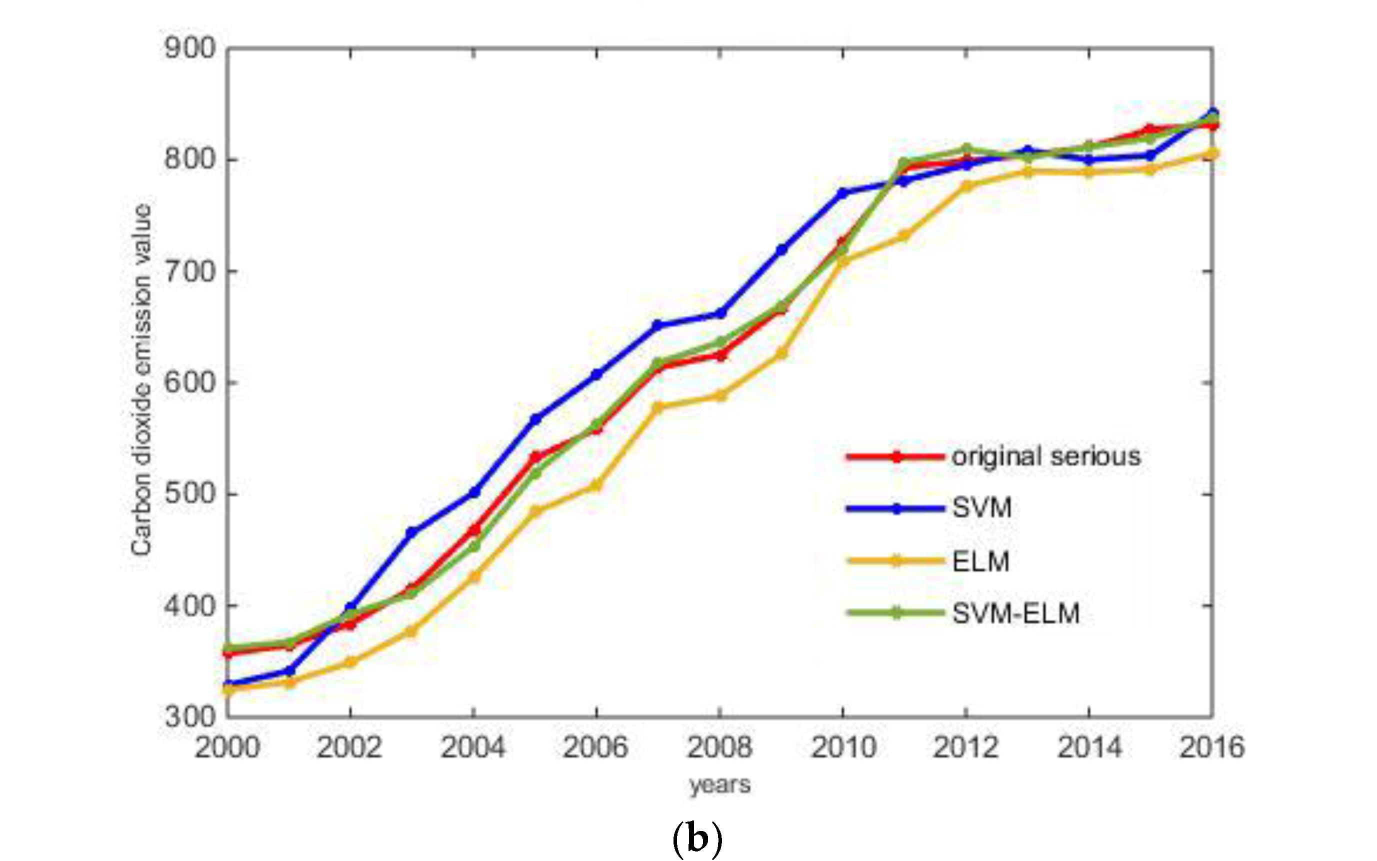
• A new forecasting model based on the extreme learning machine algorithm optimized by grey prediction theory and support vector machine is proposed. Firstly, the grey prediction theory was used to predict the amount of energy consumption in the Beijing-Tianjin-Hebei region from 2017 to 2030. Then, we used the forecasting result of the energy consumption from 2017 to 2030 as the input of the learning machine algorithm model optimized by the support vector machine to obtain the carbon emissions forecasting result in the region from 2017 to 2030. Finally, it was proven that SVM-ELM model has higher prediction accuracy than SVM model and ELM model through the analysis of empirical research.
• Because the accuracy of carbon emissions prediction is not only affected by the superiority of the algorithm, but also affected by data collection of the influencing factors, while the energy consumption is the main factor affecting carbon emissions in the Beijing-Tianjin-Hebei region, this study focused on energy consumption to forecast carbon emissions, which may not only improve accuracy but also help studying energy consumption structure and its upgradation methods.

The main structure of this article is as follows: Section 2 summarizes the principles of support vector machine algorithm, grey prediction theory and the optimized extreme learning machine algorithm, which are the theoretical basis of the study. Section 3 builds a carbon emissions prediction model based on the grey prediction theory. Based on historical data, it can predict carbon emissions from 2017 to 2030. Then its accuracy is compared with the SVM and ELM algorithm, proving that the SVM-ELM model has higher accuracy. At the same time, the forecasting result is discussed from the perspective of energy consumption structure. Section summarizes all the content of this article.

2. Materials and Methods

2.1. GM (1, 1) Forecasting Model

The grey prediction theory is used to find the laws of the system through processing raw data and establishing the corresponding mathematical model. As a result, a scientific quantitative prediction of the future state of the system is made. This theory has been applied to the research of multi-field prediction problems. GM (1, 1) is a model most commonly used by scholars which consists of a first-order differential equation that contains only univariate. It is also usually used to predict samples with a small amount of data. Therefore, we used GM (1, 1) to predict the main types of energy consumption in the Beijing-Tianjin-Hebei region from 2017 to 2030.

2.2. Basic Methodology of Extreme learning Machine Algorithm

Extreme learning machine is a new single hidden layer feed-forward neural network algorithm invented by Huang [34] which has the advantages of high speed. During the training process, we only need to set the number of hidden layer nodes. Thus, the input weights and hidden layer offsets are initialized randomly. Finally, the corresponding output weights can be obtained, which overcomes the disadvantages of local optimization of the traditional neural network algorithm and long learning time. Based on guaranteeing the learning accuracy, the speed of calculation is also improved; therefore, it has the advantages of high learning efficiency and strong fitting ability [35]. The innovation of extreme learning machines is that the training process is transformed into the solution matrix by Moore-Penrose generalized inverse problem instead of iteration. The topological structure of the extreme learning machine is shown in Figure 1.

The operation of the Extreme Learning Machine is as follows:

For a single hidden layer neural network (Figure 1), assuming there are $N$ arbitrary samples $\left(X_i,T_i\right)$, where $X_i={\left[x_{i1},x_{i2},\dots x_{in}\right]}^T\in R^n$, $T_i={\left[t_{i1},t_{i2},\dots t_{in}\right]}^T\in R^m$, a neural network with $L$ hidden layers can be expressed as:

$${\displaystyle \sum }_{i=1}^L{\gamma }_{i}f\left(W_i·X_j+b_i\right)=O_j，j=1,2\dots ,n$$

(1)

where $f\left(x\right)$ is the activation function, $W_i={\left[w_{i1},w_{i2},\dots w_{in}\right]}^T$ is input weight, ${\gamma }_i$ is output weight, and $b_i$ is the offset of the hidden layer unit.

The goal of extreme learning machine algorithm is to minimize the input error which can be expressed as:

$${\displaystyle \sum }_{j=1}^L{O}_j-T_j=0$$

(2)

where ${\beta }_i$, $W_i$ and $b_i$ must make sure:

$${\displaystyle \sum }_{i=1}^L{\gamma }_{i}f\left(W_i·X_j+b_i\right)=T_j,j=1,2\dots n$$

(3)

The matrix is expressed as:

$$M_{\gamma }=T$$

(4)

$$\begin{gathered} M\left(W_1\dots W_l,b_1\dots b_l,X_1\dots X_l\right)={\left[\begin{array}{ccc}f\left(W_1·X_1+b_1\right)& \dots & f\left(W_l·X_1+b_l\right)\\ ⋮& \dots & ⋮\\ f\left(W_1·X_n+b_1\right)& \dots & f\left(W_l·X_n+b_l\right)\end{array}\right]}_{n\times l} \\ \gamma ={\left[\begin{array}{c}{\gamma }_1^T\\ ⋮\\ {\gamma }_l^T\end{array}\right]}_{l\times m},T={\left[\begin{array}{c}{T}_1^T\\ ⋮\\ T_{\mathrm{n}}^T\end{array}\right]}_{n\times m} \end{gathered}$$

(5)

where $M$ is the output of the hidden node and $T$ is the expected output.

To train samples, $W_i$ must make sure:

$$M\left({\widehat{W}}_i,{\widehat{b}}_i\right){\widehat{\gamma }}_i-T=\underset{W,b,\gamma }{\min }M\left(W_i,b_i\right){\gamma }_i-T$$

(6)

which is equal to minimizing the loss function:

$${\displaystyle \sum }_{j=1}^N{\left({\displaystyle \sum }_{i=1}^N{\gamma }_{i}f\left(W_i·X_j+b_i\right)-T_j\right)}^2$$

(7)

Training hidden-layer neural network can be transformed into solving: $M_{\gamma }=T$ and the final output weight $\gamma$ is determined:

$$\widehat{\gamma }=M^{+}T$$

(8)

where $M^{+}$ is the Moore-Penrose generalized inverse of matrix $M$.

2.3. Basic Methodology of Support Vector Machines

The aim of SVM algorithm is to find a classification surface that can minimize the error of all training samples from the optimal classification surface instead of finding the optimal classification surface to separate samples when applied to regression fitting analysis. Many influencing factors are involved in predicting carbon emissions, so it is a linearly inseparable problem and the kernel function can be used to project the sample into the high-dimensional space and reduce the calculations at high latitudes.

For a training sample $\left(x_i,y_i\right),i=1,2,...,n$, mapping with a kernel function, the sample can be mapped to a high dimensional linear space:

$$f\left(x\right)=\omega Kernel\left(x\right)+p$$

(9)

It is hard for computer to solve the strict constraint conditions, so the relaxation factor ${\gamma }_i$ is added, and the problem is transformed into a linear programming problem of the convex function.

$$\begin{gathered} \max \left(\frac{1}{2}{\left|\omega \right|}^2\right)+C{\displaystyle \sum }_{i=1}^n{\gamma }_i \\ \mathrm{subject}\mathrm{to}{y}_i\times \left(\omega x_i+b\right)\ge 1-{\gamma }_i,{\gamma }_i\ge 0 \end{gathered}$$

(10)

Quoting Lagrange factor:

$$\mathrm{L}\left(\omega ,b,\gamma \right)=\left(\frac{1}{2}{\left|\omega \right|}^2\right)+C{\displaystyle \sum }_{i=1}^n{\gamma }_i-{\displaystyle \sum }_{i=1}^n{\alpha }_i\times \left(y_i\times \left(\omega x_i+b\right)-1+{\gamma }_i\right)-{\displaystyle \sum }_{i=1}^n{\mu }_i\times {\gamma }_i$$

(11)

Solving the derivative of Equation (11):

$$\begin{gathered} \partial \left(\omega \right)=\left|\omega \right|-{\displaystyle \sum }_{i=1}^n{\alpha }_i\times y_i\times x_i=0 \\ \partial \left(b\right)={\displaystyle \sum }_{i=1}^n{\alpha }_i\times y_i=0,{\alpha }_i\ge 0 \\ \partial \left({\gamma }_i\right)=C-{\alpha }_i-{\mu }_{i,}{\alpha }_i\ge 0,{\mu }_i\ge 0 \end{gathered}$$

(12)

To obtain the Lagrange dual problem, the problem is transformed into solving the equation ${\alpha }_i$.

$$\min \left(\frac{1}{2}{\displaystyle \sum }_{i=1}^n{\displaystyle \sum }_{j=1}^n{\alpha }_i{\alpha }_j{y}_i{y}_{j}Kernel\left(x_i\times x_j\right)-{\displaystyle \sum }_{i=1}^n{\alpha }_i\right),C\ge {\alpha }_i\ge 0$$

(13)

2.4. Primary Principal of the SVM-ELM Model for Carbon Emissions Forecasting

Because the single hidden layer map $h\left(x\right)$ in extreme learning machine algorithm has the same effect as the kernel function mapping in SVM, this study replaced the single hidden layer map $h\left(x\right)$ in extreme learning machine algorithm by Kernel function in SVM algorithm. When $h\left(x\right)$ is unknown, the following nuclear matrix is defined according to the Mercer condition [36]:

$${\Omega }_{ELM}=H{H}^T=h\left(x_i\right)h\left(x_j\right)=K\left(x_i,x_j\right)$$

(14)

Using the kernel function $K\left(x_i,x_j\right)$ can enhance the stability of the original ELM algorithm. According to the standard optimization principle, the original objective function can be expressed as:

$$\begin{gathered} \min L_p=\frac{1}{2}{\omega }^2+\frac{1}{2}C{\displaystyle \sum }_{i=1}^n{\xi }_i{}^2 \\ \mathrm{s}.\mathrm{t}.\psi \left(x_i\right)\omega =y_i-{\xi }_i，i=1,2\dots ,n \end{gathered}$$

(15)

where $C$ is a regular coefficient and ${\xi }_i$ is a training error.

According to the KKT theory (Karush–Kuhn–Tucker conditions), the above problem can be transformed into:

$$L_{p_{kelm}}=\frac{1}{2}{\omega }^2+\frac{1}{2}C{\displaystyle \sum }_{i=1}^n{\xi }_i{}^2-{\displaystyle \sum }_{i=1}^n{\eta }_i\left(\psi \left(x_i\right)\omega -y_i+{\xi }_i\right)$$

(16)

where ${\eta }_i$ is the Lagrange operator.

The output function of the SVM-ELM algorithm is:

$$\begin{gathered} \omega ={\displaystyle \sum }_{i=1}^n{\eta }_i\psi {\left(x_i\right)}^T={\psi }^T\eta \\ \mathrm{C}{\xi }_i={\eta }_i \\ \psi \left(x_i\right)\omega -y_i+{\xi }_i=0 \end{gathered}$$

(17)

where $\eta ={[{\eta }_1,{\eta }_2,...,{\eta }_n]}^T$

Defining the kernel function $K\left(x_i,x_j\right)=\psi \left(x_i\right)\cdot \psi {\left(x_j\right)}^T,i=1,2\dots n$, and SVM-ELM single hidden layer output is:

$$f\left(x\right)=\psi \left(x\right)\omega =\psi \left(x\right){\psi }^T{\left(\psi {\psi }^T+\frac{1}{C}\right)}^{-1}Y$$

(18)

Since the initial input weight and threshold of the single hidden layer of the original ELM are arbitrarily given, the algorithm is unstable. The kernel function has a strong non-linear mapping capability, which makes the SVM-ELM algorithm better approximate the function. Therefore, the SVM-ELM algorithm owns the characteristics of high learning speed, high accuracy and the generalization ability of the original model. RBF, wavelet, polynomial and other multi-core functions can be used to solve SVM. We used RBF kernel as the function.

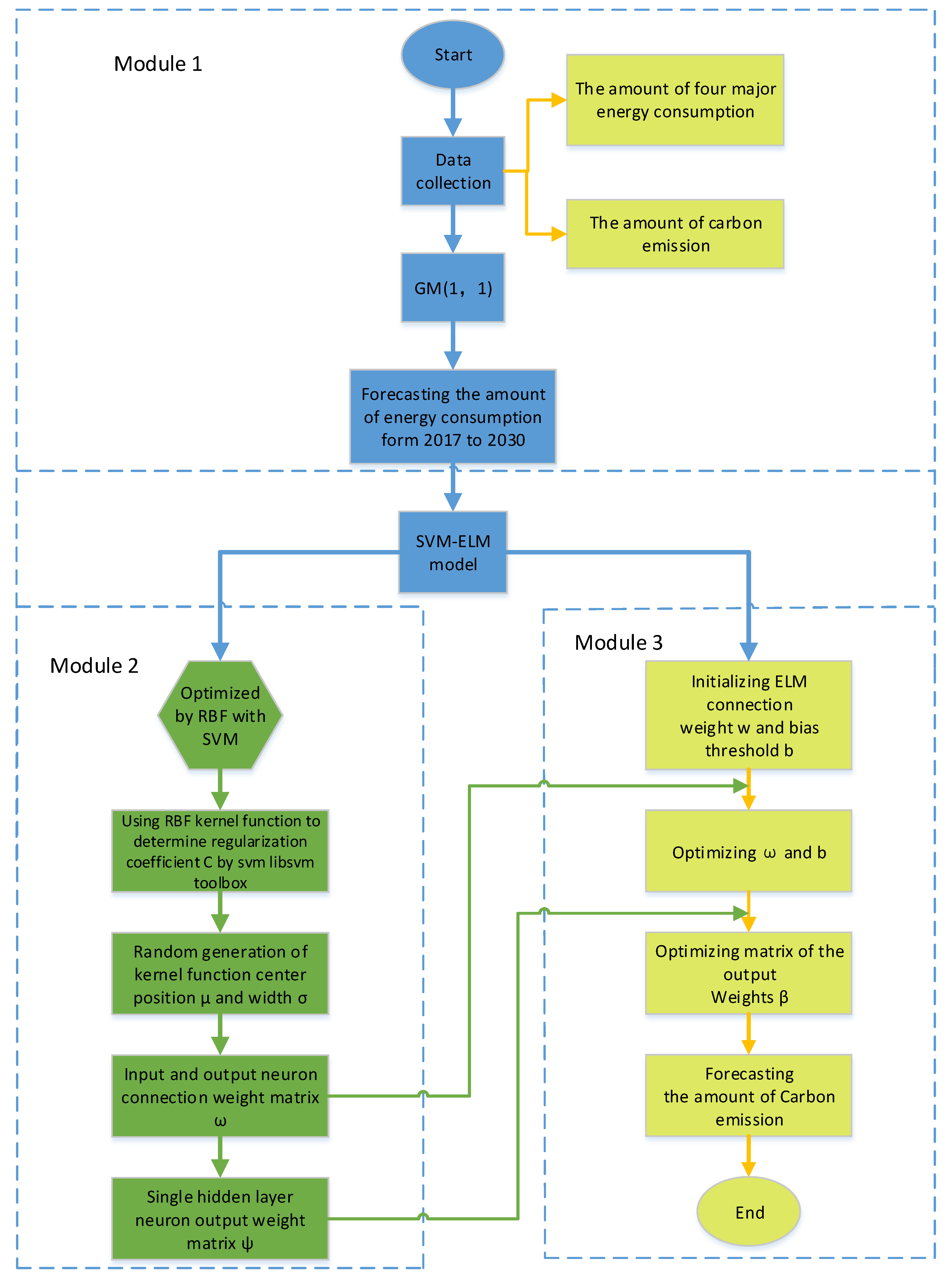
2.5. The Forecasting Model Based on Grey Prediction Theory and ELM Optimized by SVM Algorithm

Because energy consumption is the most important influencing factor of carbon emissions in the Beijing-Tianjin-Hebei region, we forecasted the amount of energy consumption related carbon emissions. The SVM-ELM model based on grey prediction was proposed to forecast the amount of carbon emissions in this region. The main steps are as follows:

(1)

Data collection and preprocessing.

We needed to collect four major influencing factors related to energy consumption: coal, petrol, natural gas and coal power. We collected carbon emissions coefficients and calculation formulas to calculate the amount of carbon emissions from 2000 to 2016 in the Beijing-Tianjin-Hebei region.

(2)

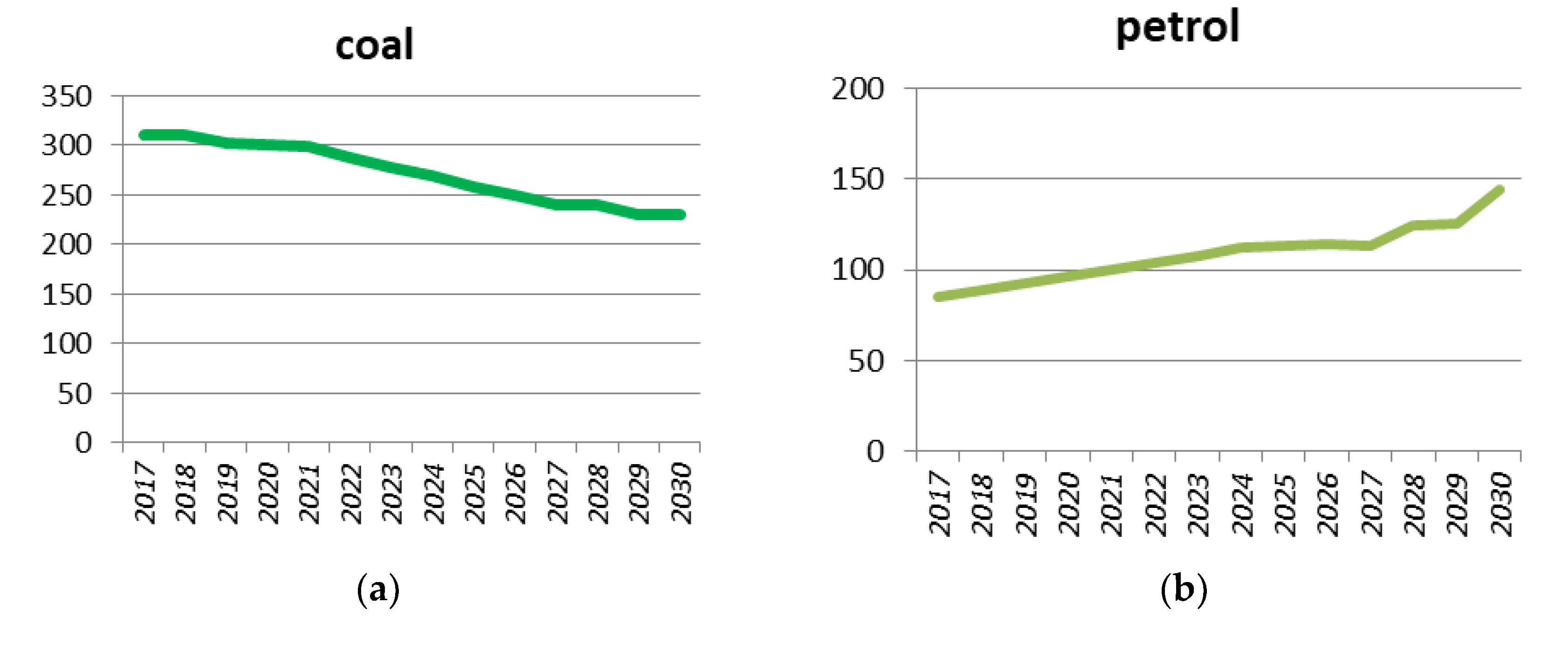
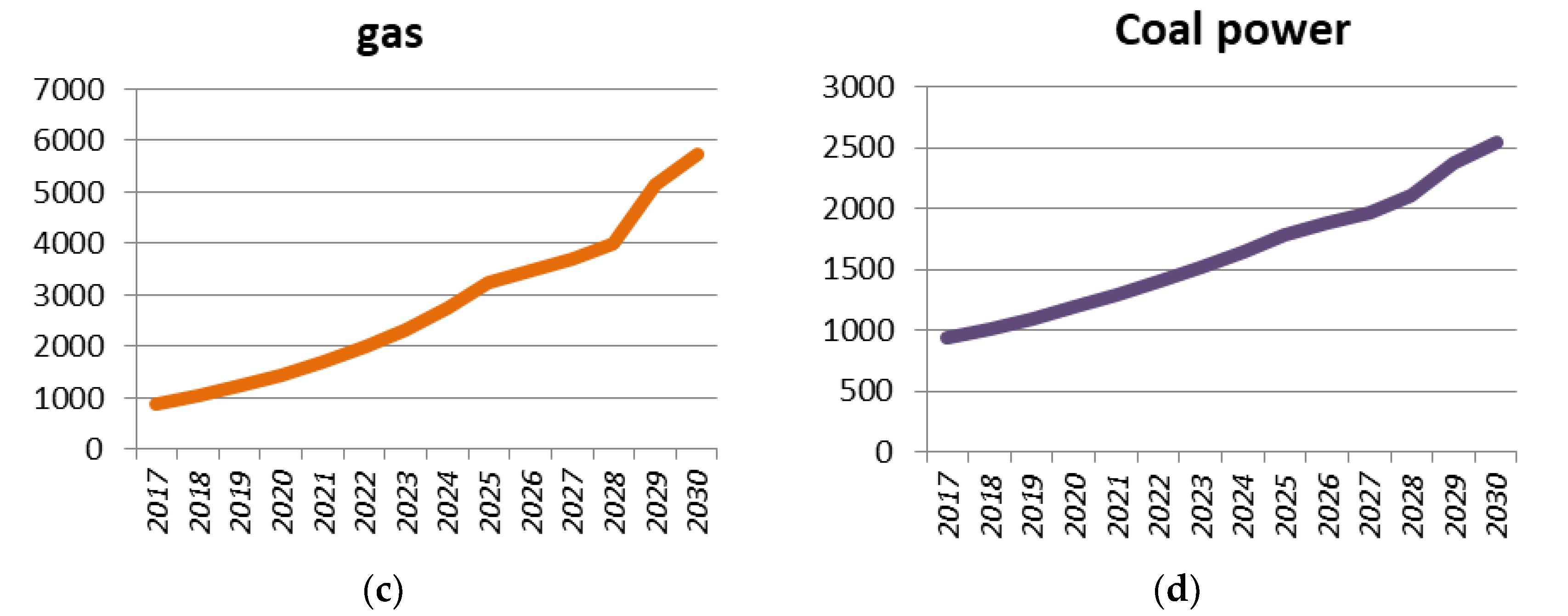
Predicting the main types of energy consumption from 2017 to 2030 in the Beijing-Tianjin-Hebei region based on the grey prediction theory.

By collecting the energy consumption from 2000 to 2016 in this region and using history data as input of the grey prediction model, the amount of energy consumption from 2017 to 2030 was forecasted.

(3)

Forecasting carbon emissions related to energy consumption in the Beijing-Tianjin-Hebei region based on SVM-ELM Model.

The four types of energy consumption and carbon emissions data from 2000 to 2010 were used as a model training set, and the data from 2011 to 2016 were used as a model test set. After a multitude of training experiments, the optimal regular coefficients and kernel function parameters were found. Therefore, the accuracy of the test set and the training set was the highest. Using the energy consumption calculated from the grey prediction model as the input of the SVM-ELM algorithm, the amount of carbon emissions related to energy consumption from 2017 to 2030 can be quickly predicted.

The flow chart of the SVM-ELM model based on grey prediction is shown in Figure 2.

3. Empirical Simulation and Data Analysis

3.1. Coefficients of Carbon Emissions Related to Energy Consumption

The 2006 IPCC Guidelines for National Greenhouse Gas Inventories [37] introduces a method to calculate carbon emissions of energy consumption. Carbon emissions produced from energy consumption mainly come from the burning of fossil fuels. Incomplete combustion of fuels often occurs during the combustion process, which makes the carbon dioxide emissions and some emissions in the form of methane monoxide or volatile organic compounds. We needed to consider the oxidation factors and coefficients of oxidation of all types of energy. For the above reasons, this study used the formulas published in the 2006 IPCC Guidelines which considered coefficients of oxidation as an important part of carbon emissions coefficients to calculate the carbon emissions in the Beijing-Tianjin-Hebei region. The specific formula is as follows:

$$E={\displaystyle \sum }_{n=1}^i{E}_i\times CE{C}_i\times NCV\times COF\times \frac{44}{12}$$

(19)

where $E_i$ is the amount of energy consumption (tons of standard coal); $CE{C}_i$ is the carbon emissions coefficient (100 million Tons/Trillion Joules); NCV is the energy low calorific value (100 million J/t); and COF is a carbon oxidation factor. Therefore, coefficients of carbon emissions consist of NCV, CEC and COF. Coefficients of carbon emissions related to energy consumption from 2006 IPCC Guidelines for National Greenhouse Gas Inventories are shown in

Table 1. Energy consumption carbon emissions coefficient.

Types	Discounted Coal Standard (kg/kg, kg/cm3)	CEC (Tons/Trillion Joules)	NCV (100 million J/t)	COF (%)
raw coal	0.7143	26.8	209.08	99.8
clean coal	0.9	25.8	263.44	99.3
liquefied petroleum gas	1.7143	17.2	501.78	99.2
refinery dry gas	1.5714	18.2	460.55	99.2
natural gas	1.33	15.3	389.31	99.4
crude	1.4286	20.0	418.16	99.4
petrol	1.4714	18.9	430.7	99.5
kerosene	1.4714	19.5	430.7	99.4
diesel	1.4571	20.2	426.52	99.3
fuel oil	1.4286	21.1	418.16	99.2
coke	0.9714	29.2	284.55	99.1
coke oven gas	0.5714	12.1	173.53	99.7
electricity	1.229	10,069 (t/GWh)	35.96 (kwh/t)	100
heat	0.03412	9.46

.

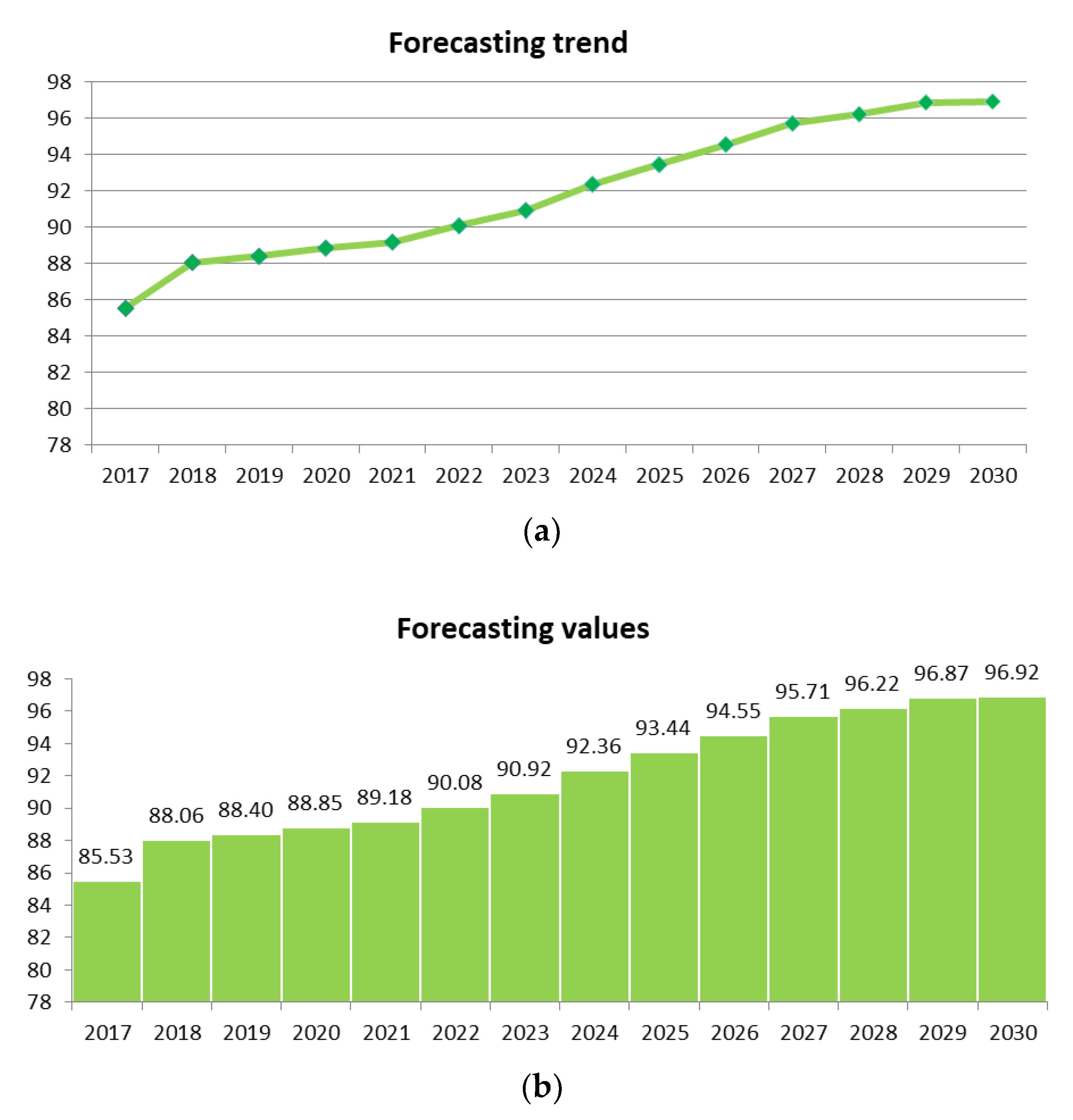
3.2. Forecasting Energy Consumption Based on GM (1, 1)

According to China Energy consumption Statistics Yearbook, this article used the amount of energy consumption in the Beijing-Tianjin-Hebei region from 2005 to 2016 as the input data of GM (1, 1). Then, we forecasted the consumption of four types of energy sources from 2017 to 2030. The forecasting results are shown in Figure 3.

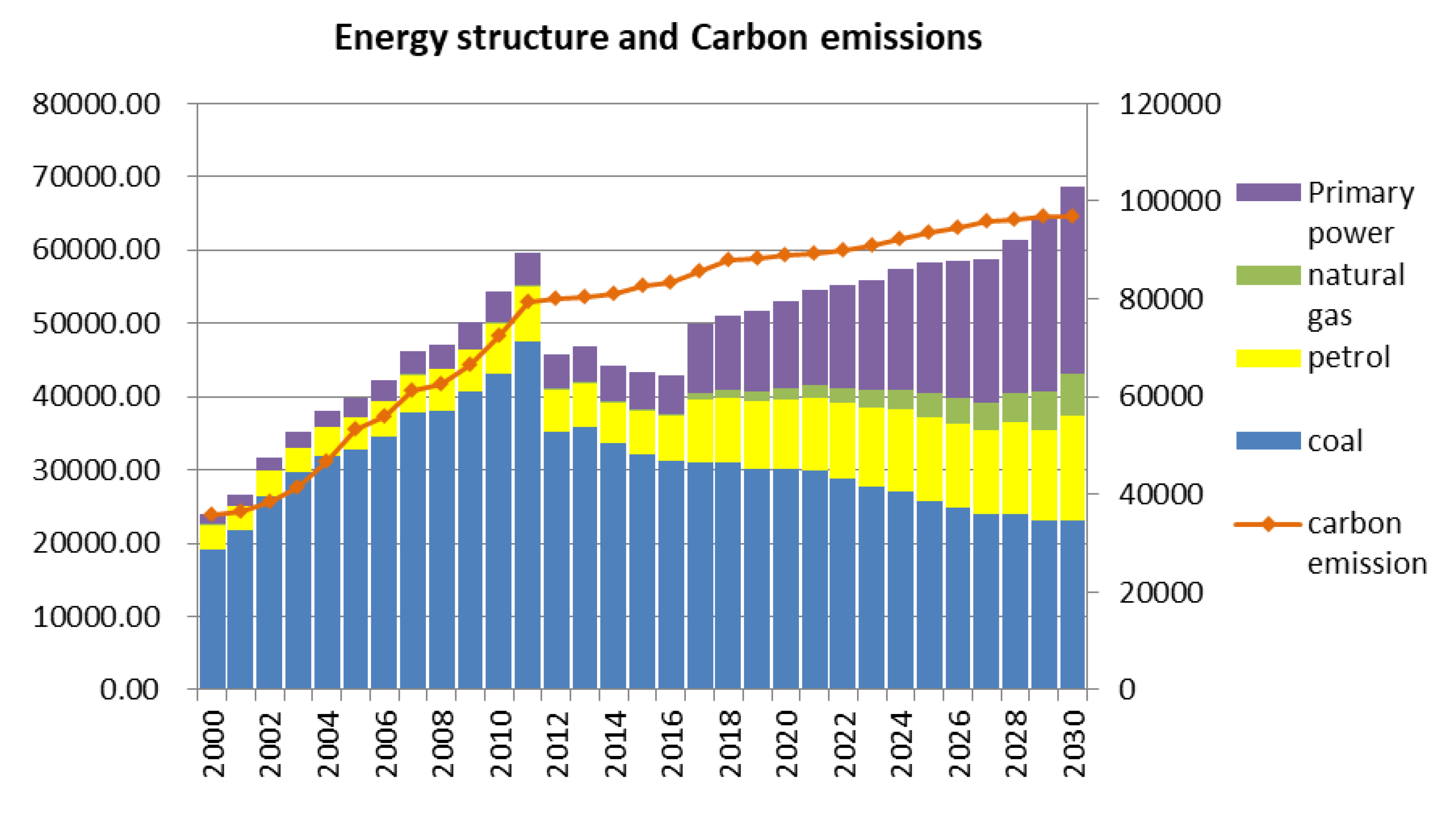
3.3. Forecasting Carbon Emissions Based on SVM-ELM Model

This study used the data for 2005–2012 as a training set and 2013–2016 as a test set. Then, we applied SVM-ELM model to forecast carbon emissions related to energy consumption in the Beijing-Tianjin-Hebei region. After 100 experiments, we found the optimal model parameters, as shown in

Table 2. SVM-ELM model parameter set.

Parameter	Value
regularization coefficient C	17
RBF kernel parameter	0.1
number of node in hidden layer	100

.

The SVM-ELM model forecasting results and comparison of forecasting results of SVM, ELM and SVM-ELM models are shown in the Figure 4.

As shown in Figure 4b, SVM-ELM model has a high accuracy for predicting energy consumption related carbon emissions in the Beijing-Tianjin-Hebei region. To prove the superiority, this article also inputted the sample to support vector machine and extreme learning machine. The forecasting results and relative errors are compared in

Table 3. RE (residual error) of each model.

Year	Actual Value	Forecasting Result	RE of SVM-ELM	RE of SVM	RE of ELM
2000	35,726.78	42,207.87	1.346569	7.935378	9.090909
2001	36,471.51	41,747.78	0.757491	6.354631	9.090909
2002	38,402.42	40,287.36	2.304398	3.551576	9.092880
2003	41,530.01	40,029.32	−1.20561	12.01801	9.092880
2004	46,828.24	45,316.87	−3.22747	7.035180	9.090909
2005	53,241.51	51,959.19	−2.40849	6.545364	9.090909
2006	55,868.82	56,310.56	0.79067	8.637444	9.090909
2007	61,360.13	63,480.21	0.68461	6.115011	5.835405
2008	62,511.46	63,623.06	1.77823	5.856977	5.891496
2009	66,640.81	69,829.08	0.43257	7.879682	6.089745
2010	72,472.94	71,993.97	−0.66090	6.311114	2.191782
2011	79,335.39	78,763.13	0.53915	1.487073	7.838322
2012	79,890.07	80,919.62	1.28871	0.438569	2.828369
2013	80,404.42	81,197.71	−0.25709	0.528436	1.765441
2014	81,132.76	82,741.96	0.01134	1.379333	2.800976
2015	82,694.21	80,743.88	−0.90735	2.781821	4.253811
2016	83,173.62	84,732.31	0.67171	1.21454	3.079388

.

To objectively compare the accuracy of a variety of models, common statistical indicators including RMSE (root-mean-square error), $R^2$ (coefficient of determination), and MRE (max relative entropy) [38] were adopted and the calculation results for the three models are shown in

Table 4. The calculation results of the three models.

Model	RMSE (100%)	${\mathit{R}}^2(100\%)$	MRE
ELM	45.2721	99.5906	7.364145
SVM	40.5655	97.9671	6.049756
ELM-SVM	12.3356	99.7780	1.623347

.

In Table 4, the results of the three indicators of the ELM-SVM model are optimal, 12.34%, 99.78% and 1.62 for RMSE, $R^2$ and MRE, respectively. The result reflects the high accuracy of the proposed forecasting model. Meanwhile, in view of RMSE and MRE indicators, the SVM model is superior to the ELM model, while, for $R^2$, the ELM model is superior.

We took the amount of energy consumption predicted by the grey prediction theory as the input of the SVM-ELM model. Therefore, the amount of carbon emissions in the Beijing-Tianjin-Hebei region from 2017 to 2030 was forecasted.

As shown in Figure 5, carbon emissions in the Beijing-Tianjin-Hebei region will gradually increase from 2017 to 2030, but the rate of increase will gradually tighten. After 2027, carbon emissions will be controlled below 97 million tons. Therefore, the government could take 100 million tons as a policy ceiling for carbon emissions by 2030. The forecasting results of this article can serve as a basis for further research on carbon emissions in the region, which means that energy consumption structure can be upgraded according to the forecasting results.

According to the forecasting results, changes in the proportion of energy consumption will affect carbon emissions, which shows the significance of energy structure upgradation. The energy structure and carbon emissions in Beijing-Tianjin-Hebei Region have been shown in Figure 6. Therefore, it is time China strengthens the application of clean energy and replaces coal with gas or other types of energy to upgrade energy consumption structure.

4. Conclusions

This article applied SVM-ELM model to forecast the carbon emissions related to energy consumption in Beijing-Tianjin-Hebei region from 2017 to 2030 after predicting the amount of four major energy consumptions, namely coal, petrol, natural gas, and coal power, by GM (1, 1) model. Energy structure upgradation and carbon emissions policy research suggestions are put forward at the end of the article. Firstly, the principles of the three algorithms ELM, SVM, and SVM-ELM were described, and the superiority of the SVM-ELM algorithm was proven in principle. Then, we used GM (1, 1) to forecast the consumption of major energy consumables from 2017 to 2030, which was used as input of the SVM-ELM model, thereby the amount of carbon emissions related to energy consumption from 2017 to 2030 was forecasted. By comparing with the prediction results of SVM and ELM algorithm, the superiority of SVM-ELM model proposed in this article was proven by empirical cases.

Due to the increasingly deteriorating environment, it is time the government to upgrade the energy consumption structure. Some policy suggestions are as follows:

(1)

First, we must accelerate the upgradation of industrial structure. The secondary industry including steel, electricity, building materials and chemical industry are key industries for energy conservation and emission reduction. Therefore, it is necessary to speed up the elimination of industries with high energy consumption and backward production capacity.

(2)

The government must develop the tertiary industry vigorously, especially the energy service industry. Since the Beijing-Tianjin-Hebei region is dominated by coal consumption, it is necessary to expand the supply of natural gas and replace coal with gas.

(3)

It is time China strengthens the use of renewable energy such as wind energy and solar energy. The government should increase subsidies for clean energy power generation and promote the trading mechanism in carbon market right now. For instance, “green certificates” can be applied to reduce the coal-fired rate of power plant, and photovoltaic technology can be actively applied in rural areas of the Beijing-Tianjin-Hebei region.

Finally, we will eventually achieve a multi-energy complementary energy consumption structure to maintain economic growth and achieve emissions reduction targets in the next step.

Although the forecasting model proposed in this article has a high degree of accuracy, the traditional gray prediction method used in the prediction of energy consumer goods has certain limitations. In future research, we will use Lagrange interpolation to reconstruct the background value, which will eliminate the traditional pull and reach a higher forecasting level. Meanwhile, we will apply the SVM-ELM forecasting model to predict carbon emissions of China’s eastern and western regions and compare results with their energy structure. Based on the results, we will deeply study the relationship between carbon emissions and energy structure by using data mining technology in the future.

References

1. Thirteenth Five-Year Plan-Integrated Work Program. Available online: http://www.sh.xinhuanet.com/2016-03/18/c_135200400_2.htm (accessed on 9 June 2018).
2. China Statistical Yearbook. Available online: http://tongji.cnki.net/kns55/Navi/YearBook.aspx?id=N2017030066&floor=1 (accessed on 6 June 2018).
3. 2017–2023 China Beijing-Tianjin-Hebei Air Pollution Control Market Research and Development Trend Research Report. Available online: http://m.chyxx.com/view/533619.html (accessed on 12 June 2018).
4. China Low Carbon Development Report in 2017. Available online: http://mini.eastday.com/mobile /180118141508633.html (accessed on 30 June 2018).
5. Cohen, S.M.; Rochelle, G.T.; Webber, M.E. Optimizing post-combustion CO2, capture in response to volatile electricity prices. Int. J. Greenh. Gas Control 2012, 8, 180–195. [Google Scholar] [CrossRef]
6. Safdarnejad, S.M.; Hedengren, J.D.; Baxter, L.L. Plant-level dynamic optimization of Cryogenic Carbon Capture with conventional and renewable power sources. Appl. Energy 2015, 149, 354–366. [Google Scholar] [CrossRef]
7. Inglesi-Lotz, R.; Dogan, E. The role of renewable versus non-renewable energy to the level of CO2 emissions a panel analysis of sub-Saharan Africa’s Big 10 electricity generators. Renew. Energy 2018, 123, 36–43. [Google Scholar] [CrossRef]
8. Ji, L.; Zhang, B.B.; Huang, G.H. GHG-mitigation oriented and coal-consumption constrained inexact robust model for regional energy structure adjustment A case study for Jiangsu Province, China. Renew. Energy 2018, 123, 549–562. [Google Scholar] [CrossRef]
9. Zhang, S.; Wang, J.; Zheng, W. Decomposition Analysis of Energy-Related CO2 Emissions and Decoupling Status in China’s Logistics Industry. Sustainability 2018, 10, 1340. [Google Scholar] [CrossRef]
10. Bo, Z.; Meng, Z.; Jun, Z. Forecasting the Energy Consumption of China’s Manufacturing Using a Homologous Grey Prediction Model. Sustainability 2017, 9, 1975. [Google Scholar] [Green Version]
11. Chen, Y.H.; Zhang, C.; He, K.J. Trend Prediction and Decomposed Driving Factors of Carbon Emissions in Jiangsu Province during 2015–2020. Sustainability 2016, 8, 1018. [Google Scholar] [Green Version]
12. Zhao, Z.D.; Hu, C.Z. Grey prediction models for the standard limit of vehicle noise. Proc. Inst. Mech. Eng. Part D J. Automob. Eng. 2018, 232, 973–979. [Google Scholar] [CrossRef]
13. Yang, J.W.; Xiao, X.P.; Mao, S.H.; Rao, C.J. Grey couple prediction model for traffic flow with panel data characteristics. Entropy. 2016, 18, 454. [Google Scholar] [CrossRef]
14. Wang, M.; Zhang, H.; Wang, X.F.; He, Y.F. A novel servo control method based on feedforward control-fuzzy-grey prediction controller for stabilized and tracking platform system. J. Vibroeng. 2016, 18, 5266–5280. [Google Scholar]
15. Gerami, M.H.; Rabbaniha, M. Forecasting the Anchovy Kilka Fishery in the Caspian Sea Using a Time Series Approach. Turk. J. Fish. Aquat. Sci. 2018, 18, 1288–1292. [Google Scholar] [CrossRef]
16. Cheng, C.H.; Yang, J.H. Fuzzy time-series model based on rough set rule induction for forecasting stock price. Neurocomputing 2018, 302, 33–45. [Google Scholar] [CrossRef]
17. Qi, R.H.; Li, D.J.; Zhang, L.Z. Performance investigation on polymeric electrolyte membrane-based electrochemical air dehumidification system. Appl. Energy 2017, 208, 1174–1183. [Google Scholar] [CrossRef]
18. Afshari, A.; Friedrich, L.A. Inverse modeling of the urban energy system using hourly electricity demand and weather measurements, Part 1: Black-box model. Energy Build. 2017, 157, 126–138. [Google Scholar] [CrossRef]
19. Matjafri, M.Z.; Lim, H.S. Prediction models for CO2 emission in Malaysia using best subsets regression and multi-linear regression. Proc. SPIE Int. Soc. Opt. Eng. 2015, 9638, 12. [Google Scholar]
20. Wang, C.C. Modelling of the compressive strength development of cement mortar with furnace slag and desulfurization slag from the early strength. Constr. Build. Mater. 2016, 128, 108–117. [Google Scholar] [CrossRef]
21. Takahashi, T.; Thornton, B.; Sato, T. Temperature based segmentation for spectral data of laser-induced plasmas for quantitative compositional analysis of brass alloys submerged in water. Spectrochim. Acta Part B At. Spectrosc. 2016, 124, 87–93. [Google Scholar] [CrossRef]
22. Zhong, Q. Prediction of energy consumption and CO2 emission by system dynamics approach. Chin. J. Eco-Agric. 2008, 16, 1043–1047. [Google Scholar]
23. Zhao, H.N.; Yu, W.Y. Research on Influence Factors of Carbon Emissions and Forecast in Hebei Province. Environ. Prot. Resour. Exploit. 2012, 807–809, 790–794. [Google Scholar] [CrossRef]
24. Fang, D.B.; Zhang, X.L.; Yu, Q. A novel method for carbon dioxide emission forecasting based on improved Gaussian processes regression. J. Clean. Prod. 2018, 173, 143–150. [Google Scholar] [CrossRef]
25. Zhao, X.; Han, M.; Ding, L.L. Forecasting carbon dioxide emissions based on a hybrid of mixed data sampling regression model and back propagation neural network in the USA. Environ. Sci. Pollut. Res. 2018, 25, 2899–2910. [Google Scholar] [CrossRef] [PubMed]
26. Wen, L.; Ma, Z.Y.; Li, Y. An investigation and forecast on CO2 emission of China: Case studies of Beijing and Tianjin. Environ. Eng. Res. 2017, 22, 407–416. [Google Scholar] [CrossRef]
27. Chang, H.; Sun, W.; Gu, X.S. Forecasting Energy CO2 Emissions Using a Quantum Harmony Search Algorithm-Based DMSFE Combination Model. Energies 2013, 6, 1456–1477. [Google Scholar] [CrossRef]
28. Sun, W.; Sun, J.Y. Prediction of carbon dioxide emissions based on principal component analysis with regularized extreme learning machine: The case of China. Environ. Eng. Res. 2017, 22, 302–311. [Google Scholar] [CrossRef]
29. Zhao, H.R.; Huang, G.; Yan, N. Forecasting Energy-Related CO2 Emissions Employing a Novel SSA-LSSVM Model: Considering Structural Factors in China. Energies 2018, 11, 781. [Google Scholar] [CrossRef]
30. Zhou, J.G.; Zhang, X.G. Projections about Chinese CO2 emissions based on rough sets and gray support vector machine. Chin. Environ. Sci. 2013, 33, 2157–2163. [Google Scholar]
31. Sun, W.; Wang, C.F.; Zhang, C.C. Factor analysis and forecasting of CO2 emissions in Hebei, using extreme learning machine based on particle swarm optimization. J. Clean. Prod. 2017, 162, 1095–1101. [Google Scholar] [CrossRef]
32. Chon, A.T.; Kim, Y.-S. Design of Fuzzy Pattern Classifier based on Extreme Learning Machine. J. Korean Inst. Intell. Syst. 2015, 25, 509–514. [Google Scholar] [Green Version]
33. Liu, H.; Mi, X.W.; Li, Y.F. An experimental investigation of three new hybrid wind speed forecasting models using multi-decomposing strategy and ELM algorithm. Renew. Energy 2018, 123, 694–705. [Google Scholar] [CrossRef]
34. Huang, G.B.; Bai, Z.; Kasun, L.L.C.; Vong, C.M. Local respective fields based extreme learning machine. IEEE Comput. Intell. 2015, 10, 18–29. [Google Scholar] [CrossRef]
35. Guo, B.X.; Li, J. Kernel extreme learning machine for indoor positioning in location finger printing. Comput. Eng. Appl. 2016, 52, 78–83. [Google Scholar]
36. Wu, J.J. Short-Term Wind Power Prediction Research Based on Extreme Learning Machine. Master’s Thesis, North China Electric Power University, Beijing, China, 2017. [Google Scholar]
37. 2006 IPCC Guidelines for National Greenhouse Gas Inventories. Available online: https://www.ipcc-nggip.iges.or.jp/public/2006gl/ (accessed on 23 June 2018).
38. Dai, S.; Niu, D.; Li, Y. Forecasting of Energy Consumption in China Based on Ensemble Empirical Mode Decomposition and Least Squares Support Vector Machine Optimized by Improved Shuffled Frog Leaping Algorithm. Appl. Sci. 2018, 8, 678. [Google Scholar] [CrossRef]
Figure 1. The topological structure of the extreme learning machine algorithm.
Energies 11 02475 g001
Figure 2. The flow chart of the forecasting model.
Energies 11 02475 g002
Figure 3. Energy consumption based on GM (1, 1): (a) coal consumption; (b) petrol consumption; (c) gas consumption; and (d) coal power consumption.
Energies 11 02475 g003aEnergies 11 02475 g003b
Figure 4. The forecasting results: (a) the comparison between original amount of carbon emissions and forecasting output of SVM-ELM forecasting model; and (b) the comparison between original amount of carbon emissions and forecasting output of forecasting model including SVM, ELM and SVM-ELM.
Energies 11 02475 g004aEnergies 11 02475 g004b
Figure 5. Forecasting values of carbon emissions: (a) the trend chart of carbon emissions from 2017 to 2030; and (b) forecasting values of carbon emissions from 2017 to 2030.
Energies 11 02475 g005
Figure 6. Energy structure and carbon emissions.
Energies 11 02475 g006