Prediction of Combustion and Heat Release Rates in Non-Premixed Syngas Jet Flames Using Finite-Rate Scale Similarity Based Combustion Models

Abstract

Generating energy from combustion is prone to pollutant formation. In energy systems working under non-premixed combustion mode, rapid mixing is required to increase the heat release rates. However, local extinction and re-ignition may occur, resulting from strong turbulence–chemistry interaction, especially when rates of mixing exceed combustion rates, causing harmful emissions and flame instability. Since the physical mechanisms for such processes are not well understood, there are not yet combustion models in large eddy simulation (LES) context capable of accurately predicting them. In the present study, finite-rate scale similarity (SS) combustion models were applied to evaluate both heat release and combustion rates. The performance of three SS models was a priori assessed based on the direct numerical simulation of a temporally evolving syngas jet flame experiencing high level of local extinction and re-ignition. The results show that SS models following the Bardina’s “grid filtering” approach (A and B) have lower errors than the model based on the Germano’s “test filtering” approach (C), in terms of mean, root mean square (RMS), and local errors. In mean, both Bardina’s based models capture well the filtered combustion and heat release rates. Locally, Model A captures better major species, while Model B retrieves radicals more accurately.

1. Introduction

Combustion of fossil fuels is still the main source of energy production. However, generating energy from combustion of conventional sources is prone to pollutant formation and emissions. Towards the down-sizing of novel energy systems, rapid mixing process is required in those operating under non-premixed combustion mode to increase heat release rates. Many engineering applications take the advantage of such turbulent combustion, which enhances the mixing of fuel and oxidizer. However, local extinction and subsequent re-ignition processes resulting from strong chemistry–turbulence interaction may occur, especially when rates of mixing exceed combustion rates, causing harmful emissions and flame instability. Extinction and re-ignition are unsteady phenomena which exhibit finite-rate chemistry effects. Since the physical mechanisms for such processes are not yet fully understood, the research is still ongoing on the subject. Due to increased computational power available today, computational fluid dynamics (CFD) is a promising tool to study such processes. Reynolds Averaged Navier-Stokes (RANS) simulations cannot be used to study complex phenomena, such as extinctions and re-ignitions, because the equations are averaged in time. Direct numerical simulation (DNS) is unfortunately limited up-to-now to low Reynolds’ numbers and simple computational setups, because it is computationally very demanding. However, DNS results can be utilized to develop/assess large eddy simulation (LES) models. LES predicts the unsteady behavior of the large scales of the flow while small scales need to be modeled. Detailed chemistry can be directly incorporated into LES of reactive flows by solving the transport equations of the filtered species. The transport equations for species $k=1\dots N_s-1$, with $N_s$ the total number of species in the kinetic mechanism, can be written as:

$$\frac{\partial (\overline{\rho }{\overline{Y}}_k^f)}{\partial t}+\frac{\partial }{\partial x_i}(\overline{\rho }{\overline{u}}_i^f{\overline{Y}}_k^f)=\frac{\partial }{\partial x_i}\left(-\overline{\rho }{D}_k\frac{\partial {\overline{Y}}_k^f}{\partial x_i}-\overline{\rho }\left({\overline{u_i{Y}_k}}^f-{\overline{u}}_i^f{\overline{Y}}_k^f\right)\right)+{\overline{\dot{\omega }}}_k,$$

(1)

where $\overline{(·)}$ represents filtered quantity in LES and ${\overline{(·)}}^f$ a Favre filtered quantity, defined as $\overline{\rho (·)}/\overline{\rho }$.

In Equation (1), $\rho \mathrm{is}\mathrm{the}\mathrm{density}\mathrm{of}\mathrm{the}\mathrm{mixture}$, $D_k\mathrm{the}$ molecular diffusion coefficient, ${\overline{Y}}_k^f$ and ${\overline{u}}_i^f$ the Favre filtered mass fraction of species k and the velocity component in i^th direction, respectively, while ${\overline{\dot{\omega }}}_k$ expresses the filtered production/consumption rate of species k, which needs to be modeled. Given a chemical kinetic mechanism of $N_s$ chemical species and $N_R$ reactions, the formation rate of species $k$, ${\dot{\omega }}_k(\mathbf{\phi })$, where $\mathbf{\phi }$ is the composition vector contains mass fractions, $(Y_1,Y_2,\dots ,Y_{N_S}),$ temperature (T)/enthalpy (h) and pressure (p), is given by [1]:

$${\dot{\omega }}_k=W_k{\sum }_{j=1}^{j=N_R}({\upsilon }_{kj}^{″}-{\upsilon }_{kj}^{\prime })R{R}_j,$$

(2)

$$R{R}_j=K_{Fj}{\prod }_{k=1}^{N_S}{(\frac{\rho Y_k}{W_k})}^{{\upsilon }_{kj}^{\prime }}-K_{Rj}{\prod }_{k=1}^{N_S}{(\frac{\rho Y_k}{W_k})}^{{\upsilon }_{kj}^{″}},$$

(3)

where $W_k$ is the molecular weight of species $k$, and ${\upsilon }_{kj}^{\prime }$ and ${\upsilon }_{kj}^{″}$ are forward and backward stoichiometric coefficients of species k in reaction $j$, respectively. $R{R}_j$ is the reaction rate of reaction $j$. $K_{Fj}$ and $K_{Rj}$ are the forward and backward kinetic constants of reaction $j$, respectively.

The problem of combustion closure in LES is to model the filtered nonlinear term ${\dot{\omega }}_k(\mathbf{\phi })$ in Equation (1) using filtered values $\overline{\mathbf{\phi }}$ available from LES solution itself. Comprehensive reviews of available LES combustion models can be found in [2,3]. Among different categories of available combustion models for LES, in finite-rate combustion models, direct detailed chemistry can be utilized by either directly solving the transport equations of species and modeling ${\overline{\dot{\omega }}}_k$, or solving the transport equations of joint velocity/composition probability density functions (PDFs) and modeling unclosed mixing term. The most adopted finite-rate combustion models are the thickened flame model (TFM) [4,5], the transported PDF (TPDF) models [6,7], the eddy dissipation concept (EDC) model [8], the Partially Stirred Reactor (PaSR) model [9,10], and the scale similarity (SS) models [11,12], each having its own pros and cons. In particular, the TFM was designed and developed mainly for turbulent premixed flames. Even though TPDF models are attractive in treating both premixed and non-premixed flames with closed ${\overline{\dot{\omega }}}_k$, their main drawback lies on their computational burden. The EDC and PaSR models were originally proposed and developed for RANS simulations (see, e.g., [13,14,15]). Although they have been used recently in LES [9,16,17,18,19], there are a few studies on the extension of these models to the LES framework. The focus of the present study is on SS models and their applications in predicting combustion and heat release rates.

In their general form, SS models are type of soft deconvolution methods [20], which use the first order approximation to reconstruct the exact field based on filtered fields. More advanced deconvolution methods are still under development for reactive flow applications [21,22]. First, Bardina et al. [23] proposed a SS model for based sub-grid scale (SGS) stress tensor. Thereby, the exact velocity field in the SGS tensor is replaced by its “grid filtered” counterpart resulting in “double grid filtered” quantities, which are exploited to model SGS stress tensor. In other words, the SGS stress tensor is replaced by the modified Leonard’s stress in Germano’s decomposition [24]. Liu et al. [25], based on decomposition of the velocity field in logarithmic bands, proposed using “test grid filtered” instead of “double grid filtered” quantities in the definition of SGS stress, which is explained in the next sections. The ability of SS models in capturing the locations where the contribution of SGS stress field is high has been proven in many studies using both a priori analysis based on DNS data (e.g., [23]), as well as experimental data (e.g., [25]). However, the drawback of the original models is their slight dissipative character. This can be explained by considering that SS models are actually low order soft deconvolution models. The issue comes from the fact that in LES the information lost by inherent grid filter is un-recoverable [26]. Thus, each soft deconvolution model needs a complementary model to handle the lost data. This is the idea behind “mixed models”, which take the advantages of both SS models and eddy viscosity type models.

In the context of LES of reactive flows, DesJardin and Frankel [11] proposed to use the SS idea to close the filtered formation rate of species ${\overline{\dot{\omega }}}_k(\mathbf{\phi })$ in Equation (1). They reported both a priori and a posteriori assessments of the method using a two-dimensional spatially developing non-premixed jet DNS database with one-step chemistry. The results (e.g., moments of product mass fraction and reaction rates) using the proposed SS models were in reasonable agreement with DNS data. Potturi and Edwards [27] also tested this model in LES of DLR and UVa combustors, but they found no improvement compared to simulation without SGS combustion model for UVa combustor. Jaberi and James [12] extended this method to dynamically evaluate the similarity coefficient. They tested the model using a DNS database of isotropic decaying compressible reacting flow and achieved results with acceptable accuracy. SS concept has further been used to develop LES combustion models in premixed flames to postulate the filtered flame surface density (FSD) in filtered progress variable balance equation [28,29]. It is evident that the direct application of SS idea in LES of reactive jets is limited in the literature to the early 2D DNS/LES spatial jet of Desjardin and Frankel [11] and 3D DNS/LES of isotropic decaying reactive flow of Jaberi and James [12], both with small LES grid filters (∆) (∆/∆_DNS = 3 in [11] and ∆/∆_DNS = 4 in [12], where ∆_DNS is the grid size used in the DNS) and single step chemistry.

In the present study, a skeletal mechanism was used to a priori assess the performance of two non-dynamic SS models (proposed in [11]) and the one developed following Liu and coworkers’ [25] idea (for SGS stress fields), using 3D DNS data. The selected SS models were employed in a more challenging test case employing large filter widths (∆/∆_DNS = 8, 12, 18) to assess their capabilities in the prediction of combustion and heat release rates along with the extinction and re-ignition phases of a temporally evolving syngas jet flame for which a DNS database is available. This DNS database is introduced in Section 2, while the SS models to be used are outlined in Section 3. An a priori analysis and the assessment metrics are explained in Section 4. The results are presented and discussed in Section 5. The paper is concluded in Section 6.

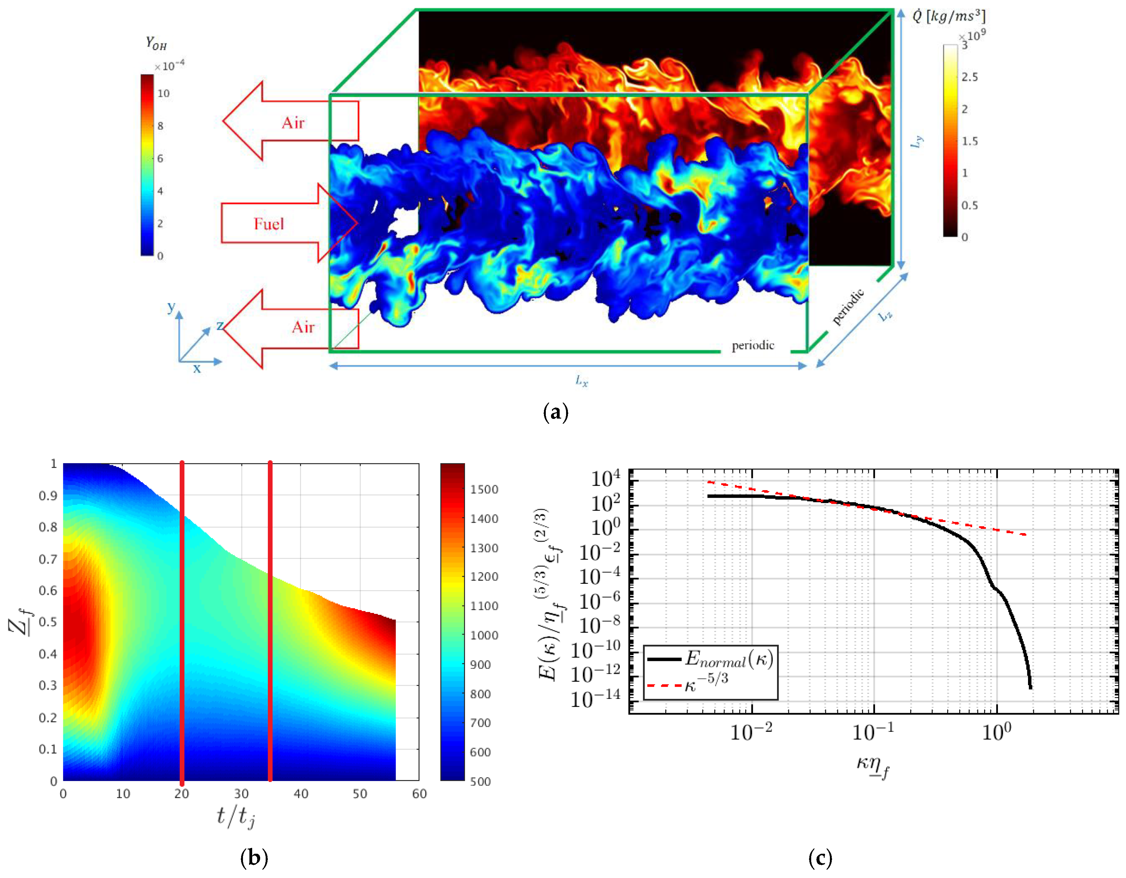
2. Direct Numerical Simulation Database

The numerical experiment used in the present work is the DNS of temporal evolution of syngas jet flame (the so-called H-case) [30]. As jets are typically encountered in various practical energy systems applications (combustors, furnaces, cooling devices, etc.), this configuration is representative of shear-driven turbulent flows that especially aims at maximizing the residence time of the fluid in the domain while enhancing the mixing process. This flame first experiences extinction up to 20$t_j$ and then re-ignition. Here, $t_j$ is “transient” jet time. It is denoted as $t_j=\mathrm{H}/\Delta \mathrm{U}=5\mathsf{\mu }\mathrm{s}$ [30], with H = 1.37 mm being the height of the initial fuel stream and ∆U = 2 × 138 m/s the difference of fuel (CO/H₂) and oxidizer (O₂/N₂) stream velocities. The adopted chemical kinetic mechanism has 11 species and 21 elementary reactions [30]. The initial jet Reynolds’ number based on initial fuel width is 9079 and the maximum turbulent Reynolds’ number achieved in the simulation is ${\mathrm{Re}}_{\mathrm{t}}=318$. The computational domain is a box with dimension 12H × 14H × 8H in x (stream-wise), y (transverse), and z (span-wise) directions, respectively. The mesh used is 864 × 1008 × 576, which results in a uniform grid size of ${\Delta }_{\mathrm{DNS}}\approx 19\mathsf{\mu }\mathrm{m}$. Periodic boundary conditions are used in x and z directions so that the flame is statistically 1D, and xz planes at each y location can be considered as statistically homogenous planes (see Figure 1a). In Figure 1b, the Favre averaged mixture fraction colored by Favre averaged temperature during the simulation is shown. As stated earlier and evident in Figure 1b, the flame experiences the transient phenomena of extinction and re-ignition. Figure 1b also reports, represented by vertical lines, the times which are used in the present study (20$t_j$, 35$t_j$) for detailed analyses. It can be inferred that the flame reignites in partially premixed mode. Figure 1c shows the normalized energy spectrum (normalized by Favre averaged Kolmogorov length scale, ${\underset{\_}{\eta }}_f$, and Favre averaged turbulent dissipation rate ${\underset{\_}{\epsilon }}_f$) obtained by velocity fluctuations on the center plane at $t=20t_j$. This figure reveals the existence of the inertial range with −5/3 law in the current case. The examination of other time instants showed the same behavior. This implies that the inertial range exists for the current configuration although it is not distinctly separated from the dissipative scales, which is common in such a low/medium Reynolds number DNS. Note that the test case has been used previously for assessment of LES combustion/mixing models [31,32,33,34,35,36,37].

3. Scale Similarity Closures for Reactive Flows

The first model of SS type, originally called scale similarity resolved reaction rate model (SSRRRM) (hereafter denoted as Model A), was proposed by Desjardin and Frankel [11]. In this model:

$${\overline{\dot{\omega }}}^A(\mathbf{\phi })=\dot{\omega }({\overline{\mathbf{\phi }}}^f)+C_A^{\overline{\Delta }}{ℒ}_{{\dot{\omega }}^A},$$

(4)

$${ℒ}_{{\dot{\omega }}^A}=\overline{\dot{\omega }}({\overline{\mathbf{\phi }}}^f)-\dot{\omega }({\stackrel{=}{\mathbf{\phi }}}^f),$$

(5)

where $C_A^{\overline{\Delta }}$ is a coefficient which can be evaluated dynamically. In the present study, a non-dynamic model has been utilized, where $C_A^{\overline{\Delta }}$ is set to one. ${ℒ}_{{\dot{\omega }}^A}$ stands for the residual field representing the SGS effects. If one filters Equation (4) and uses the same decomposition for the residual field as in Equation (4), it ends in Equation (5) for the residual field in the first filtering level. The “double grid filtered” field ($\stackrel{=}{\mathbf{\phi }})$, or more specifically the “double grid Favre filtered” field ${\stackrel{=}{\mathbf{\phi }}}^f$, is introduced (as explained in the next section).

The second model, originally called scale similarity filtered reaction rate model (SSFRRM) (hereafter denoted as Model B), stemmed from the same authors [11] and uses the filtered formation rate of filtered fields instead of resolved formation rates in the first decomposition step which results in Equation (6):

$${\overline{\dot{\omega }}}^B(\mathbf{\phi })=\overline{\dot{\omega }}({\overline{\mathbf{\phi }}}^f)+C_B^{\overline{\Delta }}{ℒ}_{{\dot{\omega }}^B},$$

(6)

where $C_B^{\overline{\Delta }}$ is the coefficient of similarity in Model B, assumed to be equal to one in the current analysis. After applying the same procedure previously described to find an expression for the residual field (${ℒ}_{{\dot{\omega }}^B})$, the following equation is obtained:

$${ℒ}_{{\dot{\omega }}^B}=\stackrel{=}{\dot{\omega }}({\overline{\mathbf{\phi }}}^f)-\stackrel{=}{\dot{\omega }}({\stackrel{=}{\mathbf{\phi }}}^f).$$

(7)

Apparently, the “double grid filtered” field is introduced for both original fields and the Arrhenius’ formation rates. In the next section, the procedure to compute these fields is explained in details. Liu et al. [25] proposed using a filter (say $\widehat{\Delta }$) larger than the grid filter ($\overline{\Delta }$) in the similarity model formulation for SGS stress field. If one uses this idea and extends it to formation rates of species, one gets the non-dynamic Model C as:

$${\overline{\dot{\omega }}}^C(\mathbf{\phi })=\dot{\omega }({\overline{\mathbf{\phi }}}^f)+C_C^{\overline{\Delta }}{ℒ}_{{\dot{\omega }}^C},$$

(8)

$${ℒ}_{{\dot{\omega }}^C}=\widehat{\dot{\omega }}({\overline{\mathbf{\phi }}}^f)-\dot{\omega }({\widehat{\overline{\mathbf{\phi }}}}^f),$$

(9)

where $\widehat{\Delta }=2\overline{\Delta }$. The non-dynamic similarity coefficient ($C_C^{\overline{\Delta }})$ is set equal to one. As can be observed, in Model C, the “test filtered” $(\widehat{\dot{\omega }})$ and “test grid filtered” fields $({\widehat{\overline{\mathbf{\phi }}}}^f)$ are introduced.

For comparison purposes, the “quasi laminar” or “no model” approach is also considered as a reference. In “no model” approach, SGS effects are neglected so that ${\overline{\dot{\omega }}}^{noModel}(\mathbf{\phi })=\dot{\omega }({\overline{\mathbf{\phi }}}^f)$.

4. A Priori Assessment and Evaluation Criteria

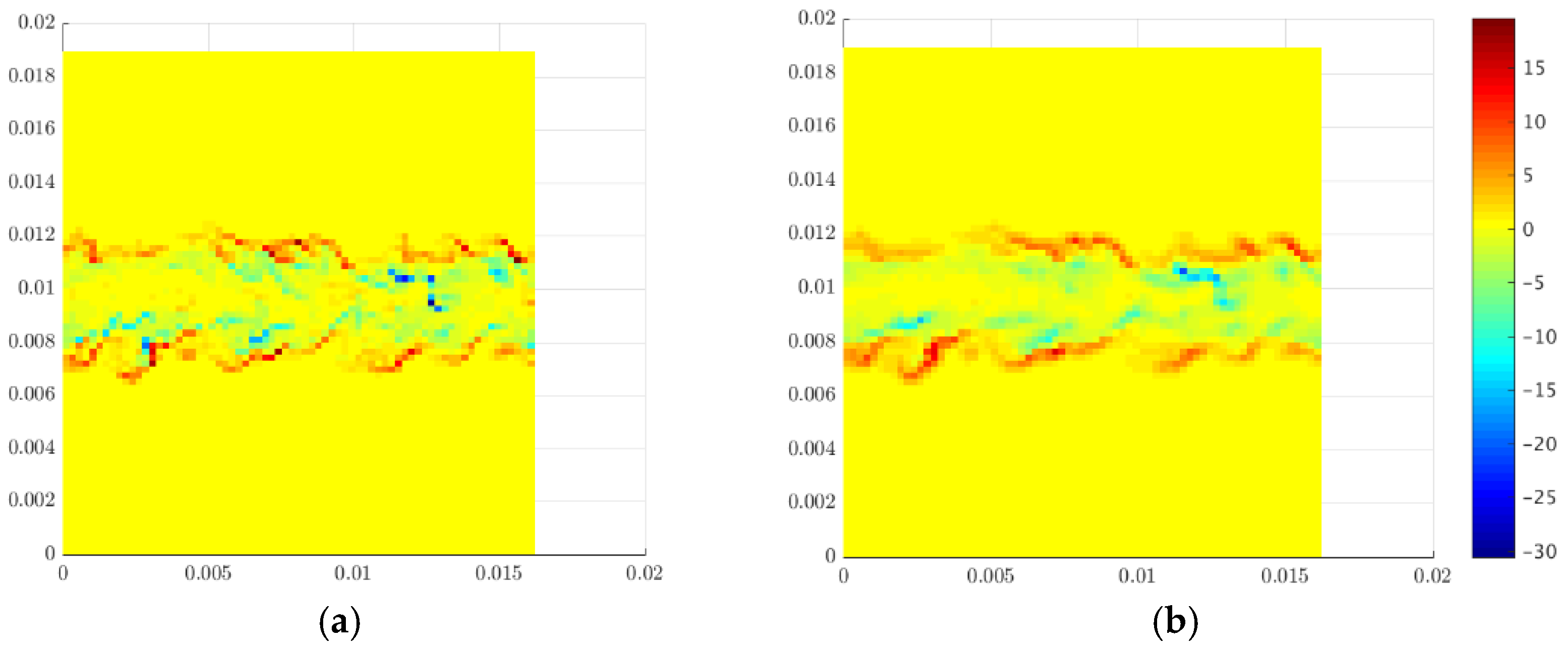
4.1. A Priori Assessment of Models Based on DNS Data

Due to development of massively large computational tools, DNS of reactive flows in low-medium range Reynolds number with detailed chemistry has become feasible. Such DNS data can be utilized to develop/assess combustion models in LES of reactive flows. Among the two main ways to utilize DNS data, namely a priori and a posteriori testing [38], an a priori analysis was adopted in this study by comparing modeled production/consumption and heat release rates with directly filtered production/consumption and heat release rates from DNS data. The modeled rates use DNS filtered quantities. With this approach, the uncertainties regarding any other models (e.g., turbulence models for stress field) are skipped and one can focus directly on the performance of the combustion model itself. The challenge in a priori analysis is that it is unable to predict the time properties of sub-grid closures [39]. A priori analyses have been performed in many previous works to study the performance of combustion SGS models [34,40,41,42,43,44]. SS combustion models have been a priori tested in 2D DNS/LES of a spatial jet [11] and 3D DNS/LES of isotropic decaying reactive flow [12], both with small LES grid filters ∆ (∆/∆_DNS = 3 in [11] and ∆/∆_DNS = 4 in [12]) and single step chemistry. In the current study, SS models (introduced in the previous section) were tested using large filter widths, in a challenging test case [30], experiencing high level of extinction and then re-ignition, relying on a skeletal chemical mechanism. In particular, since the formation rates of both major and minor species are provided by DNS, it is interesting to assess the models in predicting species formation rates of both major and radical species.

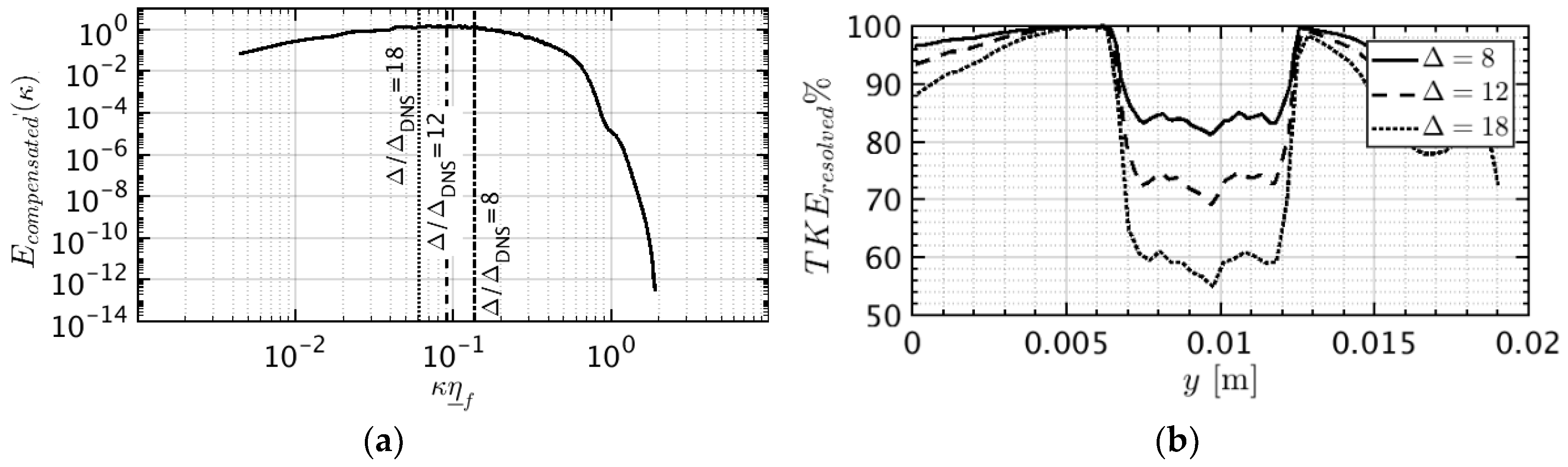
4.2. Explicit Filtering

First, the formation rates provided by DNS data are explicitly filtered in space using a top-hat filter with ∆ = 8, 12, and 18 times DNS grid size to extract the exact $\overline{\dot{\omega }}(\mathbf{\phi })$. A filtered quantity $\overline{q}$ is computed as:

$$\overline{q}=\iiint q({\mathit{X}}^{\prime })F(\mathit{X}-{\mathit{X}}^{\prime })d^3{\mathit{X}}^{\prime }.$$

(10)

Equivalently, a Favre filtered quantity is given by:

$${\overline{q}}^f=\frac{1}{\overline{\rho }}(\iiint \rho q({\mathit{X}}^{\prime })F(\mathit{X}-{\mathit{X}}^{\prime })d^3{\mathit{X}}^{\prime }),$$

(11)

where F(X) represents the 3D filter kernel which is, in this study, selected to be a top-hat filter:

$$F(\mathit{X})=F(x_1,x_2,x_3)=F(x_j)=\{\begin{array}{c}\frac{1}{{\Delta }^3}if\left|x_j\right|\le \frac{\Delta }{2}\\ 0otherwise\end{array}.$$

(12)

Therefore, Equation (10) leads to:

$$\overline{q}=\frac{1}{{\Delta }^3}{\iiint }_{-\Delta /2}^{\Delta /2}q(\mathit{X})d^3{\mathit{X}}^{\prime }.$$

(13)

A top-hat filter corresponds to the filter implicitly associated with the discretization using centered finite difference or finite volume codes which are used more often in LES [45]. The integral in Equation (13) is computed using the trapezoidal rule. In 1D, the filtered quantity $q$ in point n is computed by:

$${\overline{q}}_n^{1D}=\frac{1}{{\Delta }_{LES}}\left[\frac{{\Delta }_{DNS}}{2}\left(q\left(x_{n-\Delta /2}\right)+2{\sum }_{l=n-N/2+1}^{l=n+N/2-1}q\left(x_n\right)+q\left(x_{n+\Delta /2}\right)\right)\right],$$

(14)

where Δ is the filter width. The 3D filtered data are computed by three consecutive applications of Equation (14) in x, y, and z directions, respectively. The “test grid filtered” data are computed by application of the filter in already filtered fields using a kernel with $\widehat{\Delta }=2\overline{\Delta }$. After the data are explicitly filtered, they are interpolated to the coarse LES mesh. The scalar fields of DNS (${\phi }_k$) is first filtered/Favre filtered and then interpolated to the LES mesh. These filtered/Favre filtered interpolated data are ${\overline{\phi }}_k$ or ${\overline{\phi }}_k^f,$ which are used to evaluate SS combustion models proposed in Section 3. The required thermo-chemical properties of the filtered quantities including the new formation rates terms in SS models are computed using the OpenSMOKE++ [46] framework. For the “double grid filtered” data, the method proposed in [47] is employed. In 1D the “double grid filtered” data in point n are given by:

$${\stackrel{=}{q}}_n^{1D}=\frac{1}{8}({\overline{q}}_{n+1}+6{\overline{q}}_n+{\overline{q}}_{n-1}),$$

(15)

where $n+1$ and $n-1$ are two neighboring points. The 3D filtered data are computed by 3 consecutive applications of 1D filters in x, y and z directions.

In Figure 2a, the location of the spectral cutoff filters with the same filter width as in top-hat kernel is shown on a log-log diagram of the compensated energy spectrum. The locations of the cut off filters lie in the inertial range, which is evident by the plateau in the compensated energy spectrum.

In Figure 2b, the fraction of resolved Favre mean turbulent kinetic energy (TKE) is depicted using different filter widths. It is seen that using $\Delta /{\Delta }_{\mathrm{DNS}}=8$, more than 80% of the TKE is resolved. This fraction is reduced by increasing the filter width to 70% ($\Delta /{\Delta }_{\mathrm{DNS}}=12)$ and 60% ($\Delta /{\Delta }_{\mathrm{DNS}}=18$). This allows concluding that using the two larger filter widths is equivalent to performing very-large-eddy simulation (VLES), which is common in practical applications. The reason for applying larger filter widths compared to previous works on the same case (see [32]) is that using $\Delta /{\Delta }_{\mathrm{DNS}}=8$ in the re-ignition phase, when the flame is interacting with the decayed turbulence, the “no model” approach performs well. This means that very little can be gained by combustion models. Thus, in this situation, the test is not a challenging one to assess combustion models. This is discussed in more detail in Section 5.2.

4.3. Assessment Criteria

The first and second moments of the physical quantities are used as first metric for comparing the modeled and exact field by DNS data. Since two homogenous stream-wise (x) and span-wise (z) directions exist, the first moment is defined as the planar average (on xz planes) at different crosswise (y) heights. The average is denoted by $\underset{\_}{(·)}$. The second moment is the “root mean square (RMS)”, which is computed for an arbitrary quantity “q” as:

$$q_{RMS}=\sqrt{\underset{\_}{{(q-\underset{\_}{q})}^2}}.$$

(16)

Furthermore, to sum-up the local incurred errors and get one value from the whole sample space, the cumulative relative error is defined as below:

$$ϵ=\frac{\Vert {\dot{{\omega }_k}}^{model}({\overline{\mathbf{\phi }}}^f)-{\overline{\dot{{\omega }_k}(\mathbf{\phi })}\Vert }_2}{{\Vert \overline{\dot{{\omega }_k}(\mathbf{\phi })}\Vert }_2},$$

(17)

where ${\Vert .\Vert }_2$ is the L-2 norm with ${\dot{{\omega }_k}}^{model}({\overline{\mathbf{\phi }}}^f)$ the estimator and ${\overline{\dot{\omega }}}_k(\mathbf{\phi })$ the exact filtered DNS data. The sample space includes the clipped data from DNS domain. The data are confined to a region where ${\underset{\_}{Z}}_f\ge 0.02$ with ${\underset{\_}{Z}}_f$ expressing the Favre mean mixture fraction. This is done to avoid nearly zero values of net formation rates in the regions outside the flame brush.

Beside the filtered reaction rates in Equation (1), the filtered heat release rate in the filtered energy equation is also of great importance. In sensible enthalpy ($h_S)$ form, the balance of energy reads:

$$\frac{\partial (\overline{\rho }{\overline{h}}_s^f)}{\partial t}+\frac{\partial }{\partial x_i}(\overline{\rho }{\overline{u}}_i^f{\overline{h}}_s^f)+\frac{1}{2}\frac{\partial (\overline{\rho }{\overline{u}}_j^f{\overline{u}}_j^f)}{\partial t}+0.5\frac{\partial }{\partial x_i}\partial (\overline{\rho }{\overline{u}}_j^f{\overline{u}}_j^f{\overline{u}}_j^f)=\frac{\partial }{\partial x_i}\left(\overline{\rho }{\alpha }_k\frac{\partial {\overline{h}}_s^f}{\partial x_i}-\overline{\rho }({\overline{u_i{h}_s}}^f-{\overline{u}}_i^f{\overline{h}}_s^f)\right)+\frac{\partial \rho }{\partial t}\overline{\dot{Q}},$$

(18)

where ${\alpha }_k=\raisebox{1ex}{$\lambda $}\!\left/ \!\raisebox{-1ex}{$\overline{\rho }Cp$}\right.$ is the thermal diffusivity with $\lambda$ the thermal conductivity. The unclosed filtered heat release rate ($\overline{\dot{Q}}$) contains the cumulative effect of all filtered species source terms and it is computed as:

$$\overline{\dot{Q}}=-{\sum }_{k=1}^{N_s}\Delta h_k^0{\overline{\dot{\omega }}}_k,$$

(19)

where $\Delta h_k^0$ is the enthalpy of formation of species k. To compute the exact $\overline{\dot{Q}}$, the quantity $\dot{Q}$ from DNS is directly filtered. For the modeled $\overline{\dot{Q}}$, ${\dot{{\omega }_k}}^{model}({\overline{\mathbf{\phi }}}^f)$ from different models is used in Equation (19).

5. Results and Discussion

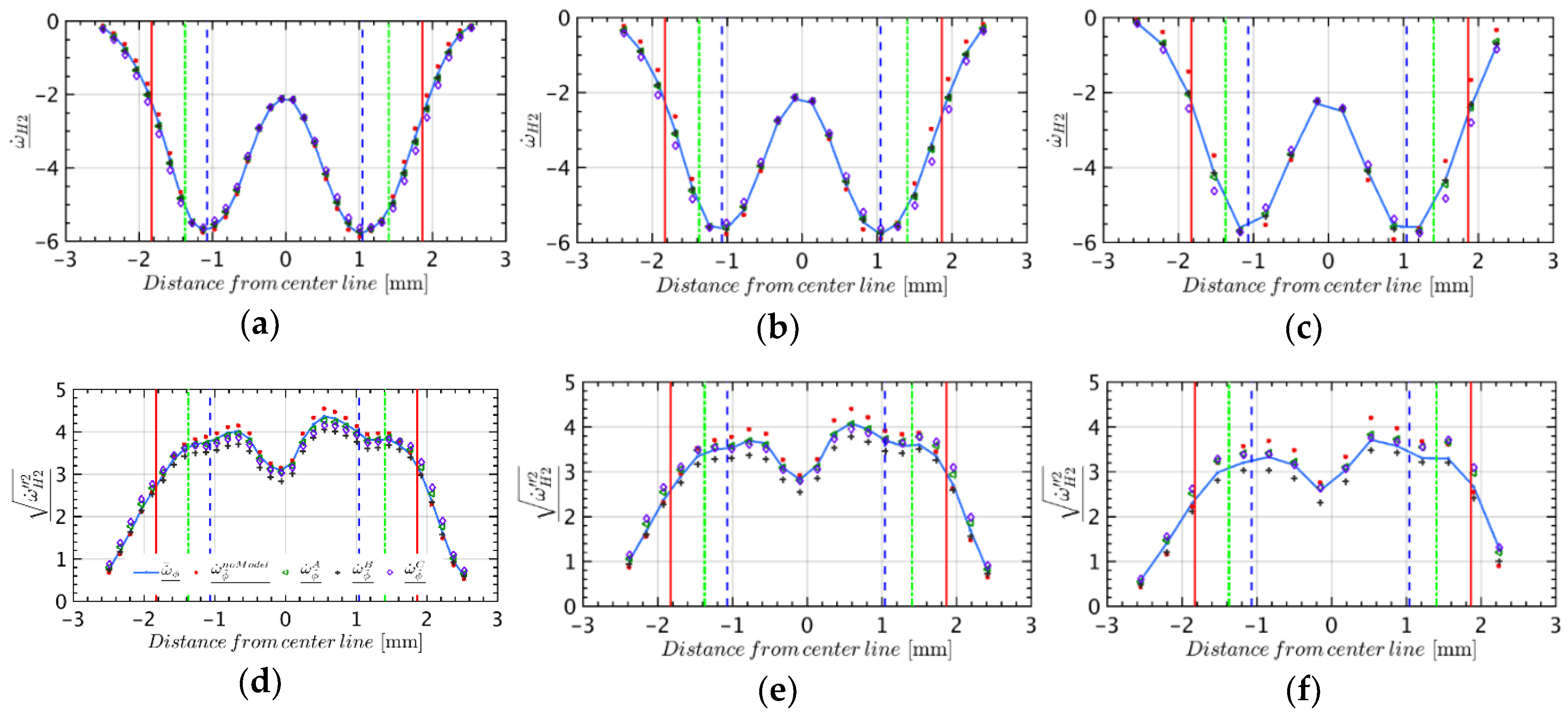
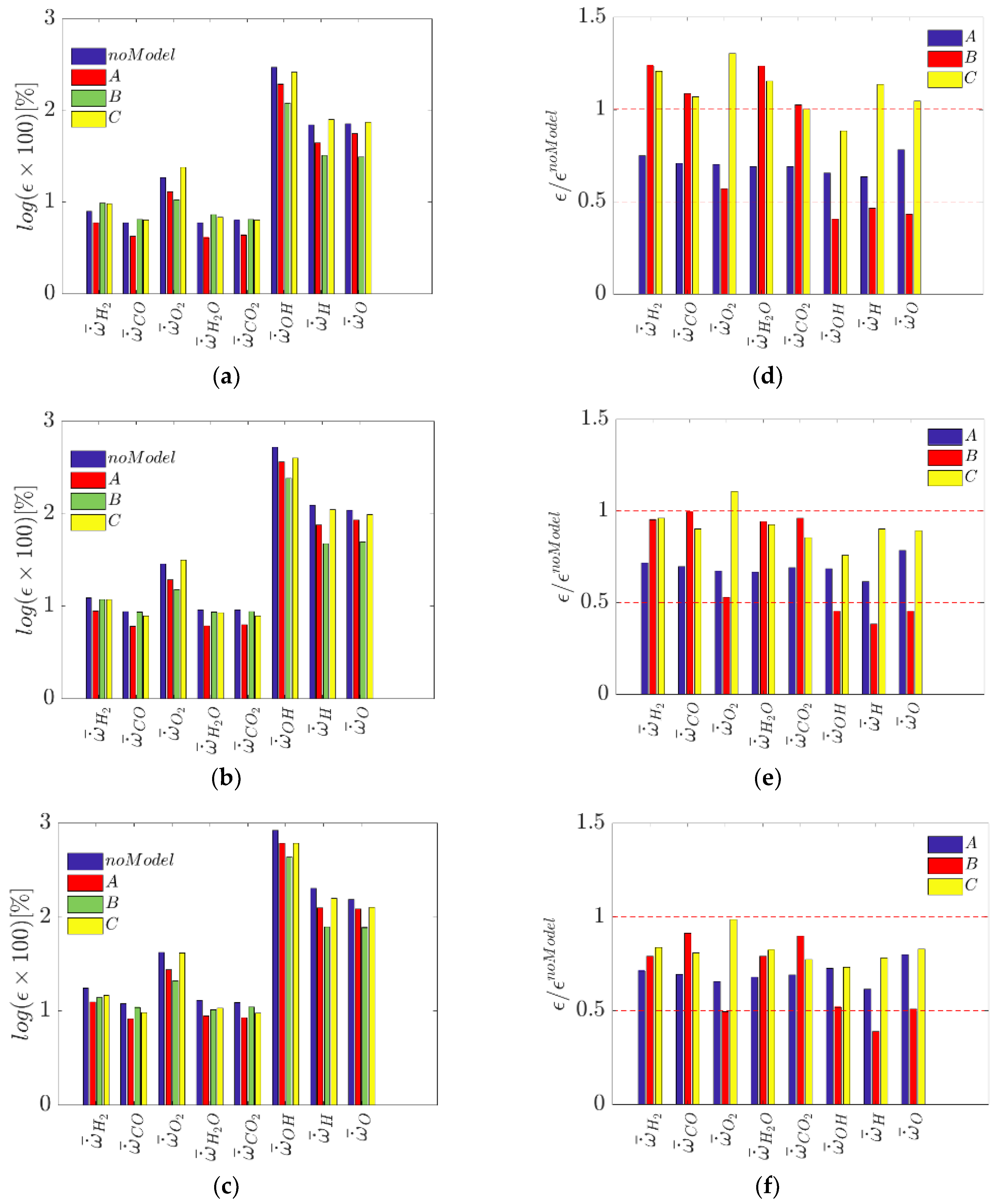
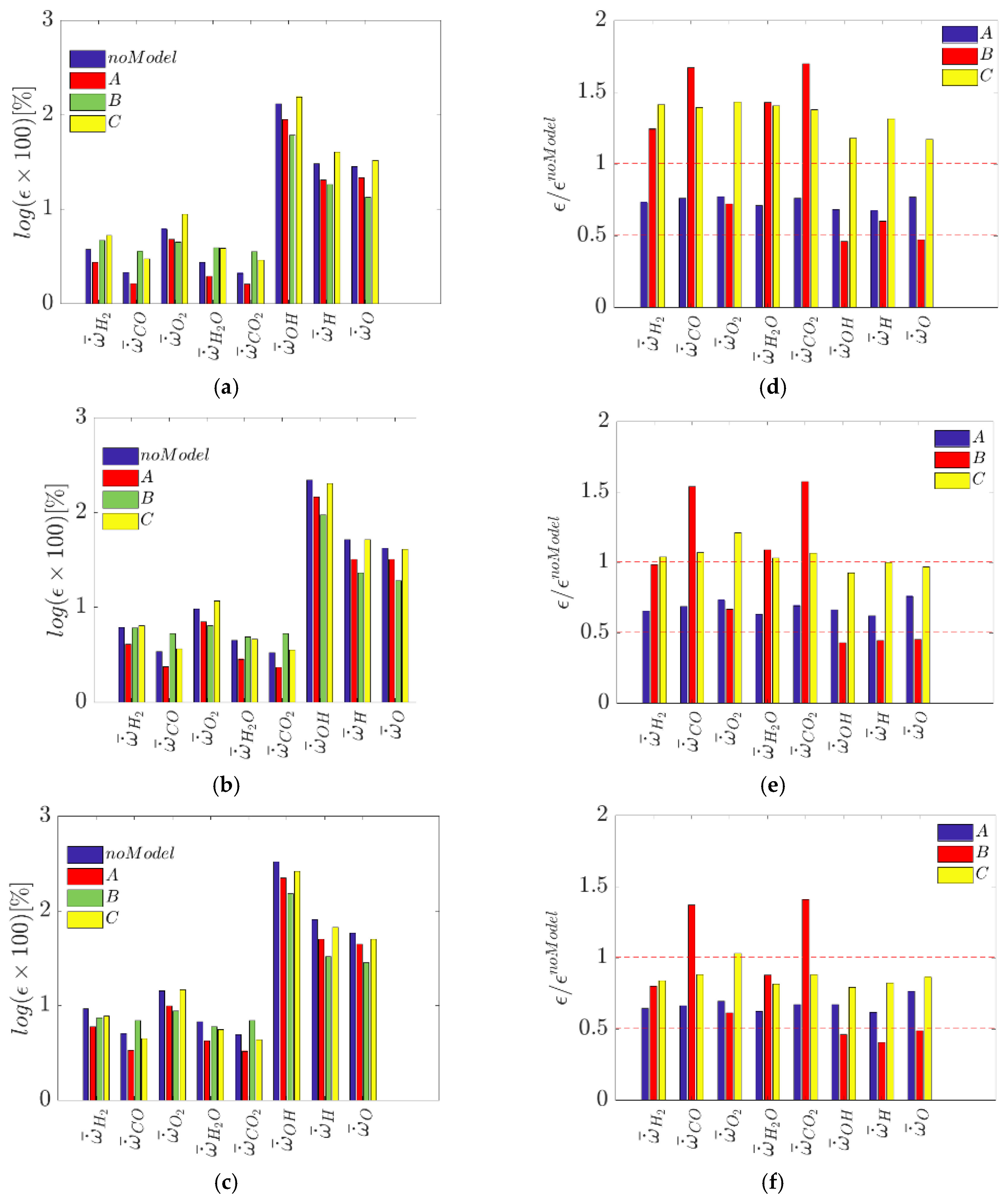
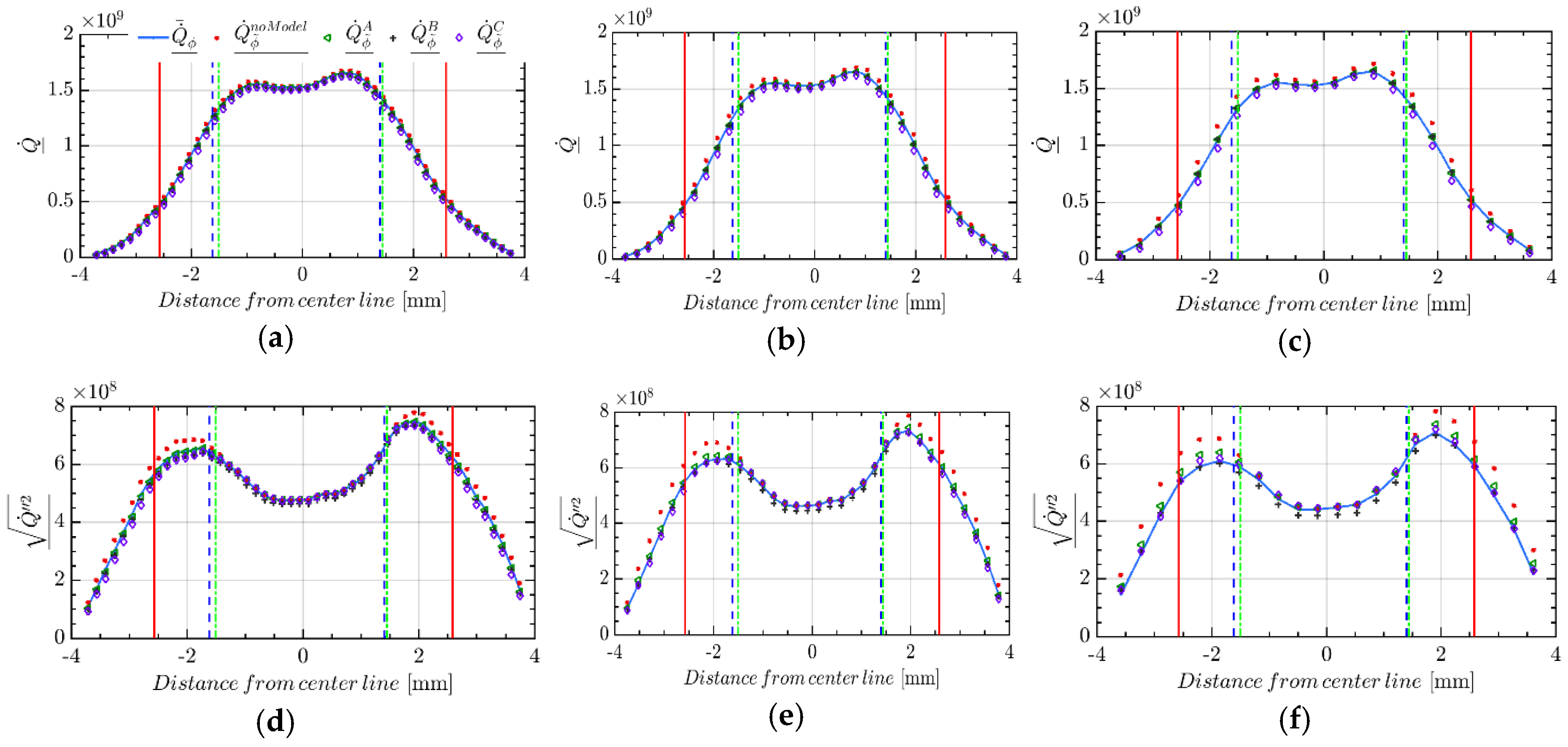
5.1. Combustion Rates Predictions in Extinction Time

In this section, the data at the times at which the flame experiences maximum local extinction is analyzed. At $t=20t_j$, the flame is in the fully turbulent, self-similar regime [48]. In Figure 3, the ability of the three SS models in predicting the filtered consumption rate of H₂ (fuel) is compared with the exact filtered reaction rate ${\overline{\dot{\omega }}}_{H2}(\mathbf{\phi })$ obtained from DNS database. The “quasi laminar” or “no model” approach is also shown as reference. In “no model” approach, SGS effects are neglected and ${\dot{\omega }}_{CO}^{noModel}(\mathbf{\phi })=\dot{\omega }({\overline{\mathbf{\phi }}}^f)$. The analysis is done for three different filter widths. From left to right, the filter size increases from $\Delta /{\Delta }_{\mathrm{DNS}}=8$ to $\Delta /{\Delta }_{\mathrm{DNS}}=12$ and $\Delta /{\Delta }_{\mathrm{DNS}}=18$. Top figures compare the first moments (mean) and the bottom figures compare the second moments (RMS). The data are clipped to a region where ${\underset{\_}{Z}}_f\ge 0.02$ with ${\underset{\_}{Z}}_f$ expressing the Favre mean mixture fraction.

In Figure 3, it is shown that all of the analyzed models, including the “no model” approach, can capture qualitatively the consumption rate of fuel in terms of both mean and RMS. Looking at mean results, in the core jet region, all models produce similar results. However, by approaching the plane of maximum mean TKE (the vertical blue dashed line) deviations and differences become higher. For $\Delta /{\Delta }_{\mathrm{DNS}}=8$ (Figure 3a) the “no Model” approach results in slightly higher/lower mean consumption rates. It can be observed in Figure 3a–c that the difference compared to the exact value (blue lines) increases by increasing the filter width. For example, in Figure 3c, the “no model” approach results start to deviate from the exact filtered DNS values in the first plane located after the central plane (y = 0). However, by using smaller filter width (see Figure 3a), the “no model” approach can predict the mean in a broader spatial range. Models A and B produce almost the same mean profiles and the error is lower than that of the other two models, i.e., Model C and the “no model” approach. Looking at RMS profiles, in Figure 3d–f, the “no model” approach reveals errors. Considering that the “no model” approach has error both in mean and the RMS profiles, one can conclude that a model needs to account for SGS effects. For the species here analyzed, this observation is more pronounced when using filter widths larger than $\Delta /{\Delta }_{\mathrm{DNS}}=8$.

It should be mentioned that the same behavior is observed for other major species, where Model C and the “no model” approach failed to predict the true spatial mean values while Models A and B predicted almost the same mean in a good agreement with the filtered DNS data.

In Figure 4, the results of the performance of SGS models in predicting filtered formation rate of H radical are analyzed. It should be noted that the mean formation rate of H is very low, since the flame is experiencing high level of local extinction. The H radical is locally produced in the pockets of burning gases and also in the burning surfaces around the extinction holes [49]. Large errors are seen using the “no model” approach and Model C in predicting the mean ${\overline{\dot{\omega }}}_H$. Considering the mean, both Models A and B are in good agreement with DNS results. In terms of RMS in Figure 4d–f, the best performance is obtained with Model B. It is interesting to observe how SS Models A and B can preserve the mean even using a large filter width $\Delta /{\Delta }_{\mathrm{DNS}}=18$.

In Figure 5, different models for different species and filter widths are assessed based on their local errors using the cumulative local error metric. First, as expected, locally, the error increases with increasing the filter width for all species. Second, looking at major species, it is seen that the performance of Models B and C is improved compared to the “no model” approach by increasing the filter width (see Figure 5a,c). It seems that, locally, the two models are more effective using larger filter widths. The cumulative local error of the “no model” approach is not much higher than that of other models and for some species less than Model C (see, e.g., Figure 5a for O₂ and H₂O). However, one cannot conclude about the performance of models by only looking at the local errors. The results should be used together with the first and second moments statistics. For example, although Model B predicts higher local errors compared to the “no model” approach for H₂ species using $\Delta /{\Delta }_{\mathrm{DNS}}=8$, the mean of ${\overline{\dot{\omega }}}_{H_2}$ is in a very good agreement with filtered DNS data (see Figure 3a). It can be concluded that the SS Model B produces data with the same mean as the exact filtered DNS, but with higher deviations. Third, looking at radicals, local errors are much higher than that for major species. The prediction for the OH is the worst. This is the result of errors in both mean and RMS profiles.

Model A, independently of the filter width, results in the lowest cumulative local error for all major species except O₂. It is reasonable to conclude that, since Model A predicts the mean with a good accuracy (see, e.g., Figure 3) and the lowest local errors, this model is preferable for major species.

Looking at radicals, Model B has the least local error. Considering that Model B has high accuracy in predicting mean of the radicals’ net formation rates, it can be concluded that Model B is a better model to capture radical net production/consumption rates. Detailed analysis of the rate of reactions (Equation (3)) involved in the syngas mechanism shows that O₂ is mainly consumed through H + O₂ = O + OH and H + O₂ (+M) = HO₂ (+M) reactions. The contribution of all other reactions is very small. As a result, O₂ net consumption rate is linked to radical formation rates. Since Model B is the best model to capture radicals net formation rates, the same is true for O₂.

Further, in Figure 5d–f, the performances of different SS models are compared with the “no model” approach by dividing their cumulative local errors to the one of “no model” approach. The value of 1 in this figure shows that the models have the same cumulative local error as the “no model” approach. It is now clearly seen that Models B and C are filter dependent, i.e., increasing the filter width decreases their local error values compared to the “no model” approach. However, the relative performance of Model A remains approximately constant. It is observed that the sum of local errors approximately improved by 25% using Model A. For radicals, it is evident that Model B has the best performance by decreasing the errors more than 50% compared to using no SGS model for combustion.

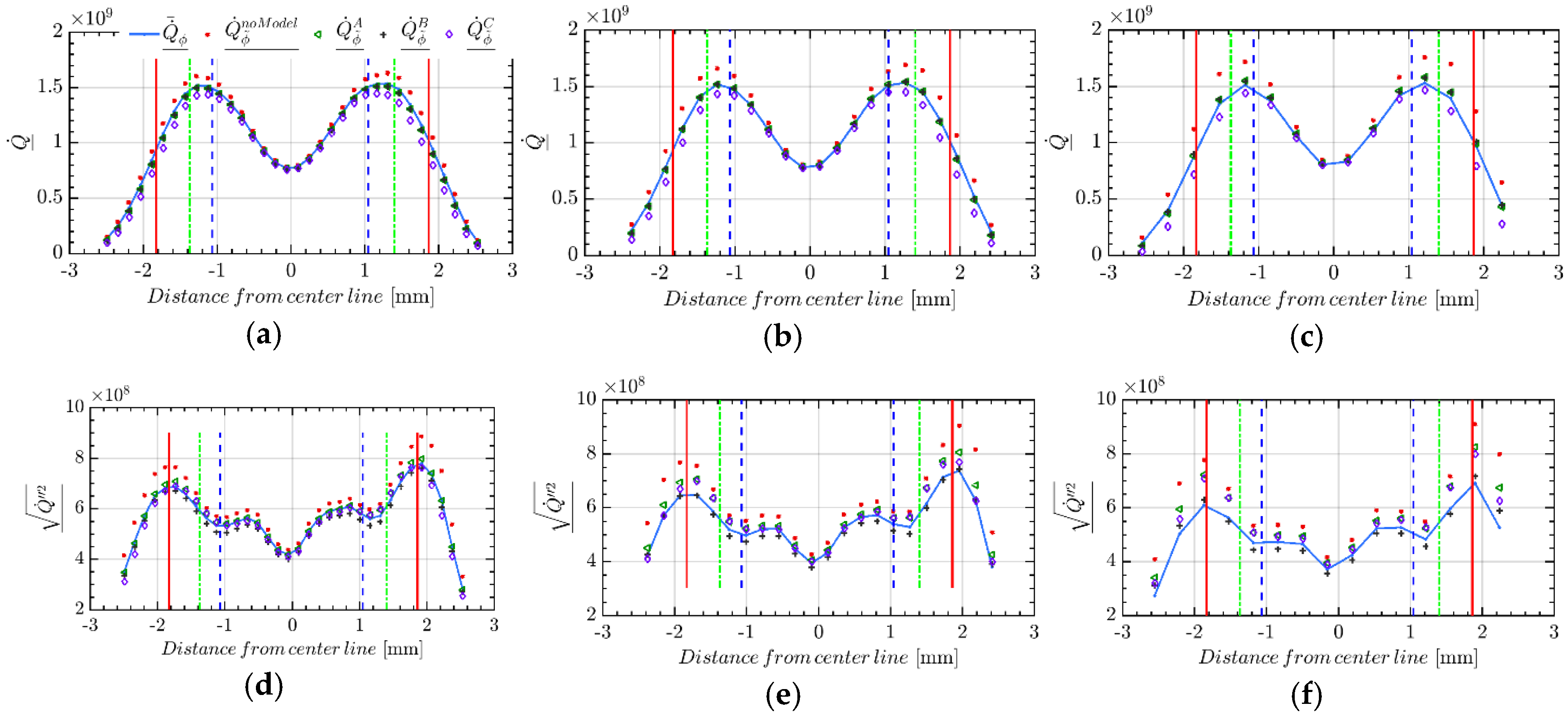
5.2. Heat Release Rates Predictions in Extinction Time

Concentrating now on the filtered heat release rate in energy equation, Figure 6 depicts the mean and RMS of filtered heat release rates per unit volume computed using different models and filter widths. It should be noted that, to compute $\underset{\_}{\overline{\dot{Q}}}$ (mean of the filtered heat release rate), $\dot{Q}$ from DNS is first directly filtered and afterwards the mean is determined, as described in Section 4.3. To get the heat release rates from the models, the related modeled $\overline{{\dot{\omega }}_j}$, respectively, from Equations (4), (6) and (8), is inserted into Equation (19).

In Figure 6a–c, the failure of the “no model” approach to predict the correct mean heat release rate is observed. It can be concluded that, without using SGS combustion model in the current case, the amount of local extinctions is not correctly captured. Higher prediction of heat release rate means that the lower number of computational cells are predicted to be in extinction mode. On the contrary, Models A and B can predict the mean filtered heat release rates with a very good accuracy. As expected, the predictions of Model C are not satisfactory.

5.3. Combustion Rates Predictions in Re-Ignition Time

The same analysis proposed in Section 5.1 is repeated here for the time at which the flame experiences re-ignition from the core region of the jet. The flame interacts with fully developed decaying turbulence at this time instant [48].

In Figure 7 the modeled filtered rate of consumption of H₂ (fuel) is compared with the exact values obtained by filtering the DNS data. In Figure 7a,d, it is evident that, for a small filter width ($\Delta /{\Delta }_{\mathrm{DNS}}=8)$, all models predict almost the same mean and RMS. Moreover, the error of using no SGS model is very low. This shows that, for the current time instant/regime, by using $\Delta /{\Delta }_{\mathrm{DNS}}=8$, in mean, the interaction of turbulence and chemistry is not high. SGS effects are negligible and filtered production/consumption rate of fuel can be evaluated by using filtered scalar fields. It should be considered that $\Delta /{\Delta }_{\mathrm{DNS}}=8$ admits the criteria of Pope [50] (see Figure 1a) for TKE resolution, however, if one wants to assess the performance of combustion models in the current case, it is needed to increase the filter width to see the effects of unresolved flame in mean filtered production/consumption rate of fuel. By using $\Delta /{\Delta }_{\mathrm{DNS}}=8$ and looking at mean filtered fuel net formation rate (Figure 7a), one can only conclude that the SGS combustion models which are tested can adapt themselves to the condition that there is no need to do SGS modeling. In other words, they can switch themselves off automatically. In the current study two larger filter widths are also applied. By increasing the filter width, the “no model” approach error increases slightly in both mean and RMS (see Figure 7c,f), although it can still predict the profile qualitatively. This is also true for other three models, however the increase of the error is less for SS models. It should be mentioned that, for other major species, e.g., CO, O₂, CO₂ and H₂O, the same performance as described in Figure 7 for H₂ is observed. Thus, for the sake of brevity, only the results for ${\dot{\omega }}_{H2}$ are presented.

Filtered H radical production/consumption rate is analyzed in Figure 8. Compared to Figure 4, it is evident that the flame is in re-ignition phase, where the rate of production of H radical increased in the core of the jet. The maximum error of the “no model” approach is around the mean stoichiometric plane and the region between this plane and the maximum of mean temperature fluctuations. In the core of the jet, the “no model” approach can predict the true mean regardless of the applied filter width. It seems that, in the core jet region, due to perfect mixing and the lack of gradients, the flame is in “perfectly stirred reactor” [1] regime.

Contrary to the “no model” approach, the SS Models A and B predict the mean formation rate ${\overline{\dot{\omega }}}_H$ with good accuracy regardless of the applied filter width. Similar to Figure 4, Model C fails to predict the mean with good accuracy.

In terms of the second moment, all models predict the qualitative behavior. The deviation from the exact RMS increases by increasing the filter width. Similar to previous observations with respect to radicals in the current study, Model B better predicts the RMS of H radical compared to other models.

In Figure 9a–c, models are assessed based on their local results compared to the “no model” approach. As shown, by using $\Delta /{\Delta }_{\mathrm{DNS}}=8$ (Figure 9a), the “no model” approach performs with a reasonable error and interestingly with local errors less than Models B and C for some species. The least local error is realized by Model A in agreement with the results for major species in the previous subsection in the instant of maximum local extinction. Further, the relative behavior of Model A remains the same when the filter width increases. The results of Models C and B show the dependency to the filter width. The local error incurred by using these two models for some species are first higher than the “no model” approach (see Figure 9a for H₂ and O₂). They become less than it is in Figure 9c, where the filter width increases. Similar to Figure 5, the error in prediction of radicals is much higher than that for major species. Compared to results in extinction time (Figure 5), the cumulative local errors are lower. It is revealed that the turbulence–chemistry interaction is lower in re-ignition than the extinction time. Further, in Figure 9d–f, the relative performances of different SS models compared to the “quasi laminar” or “no model” approach are shown. Compared to Figure 5d–f, the same behavior is observed for Model A, i.e., improvement of approximately 25% for major species and radicals independent of filter width applied.

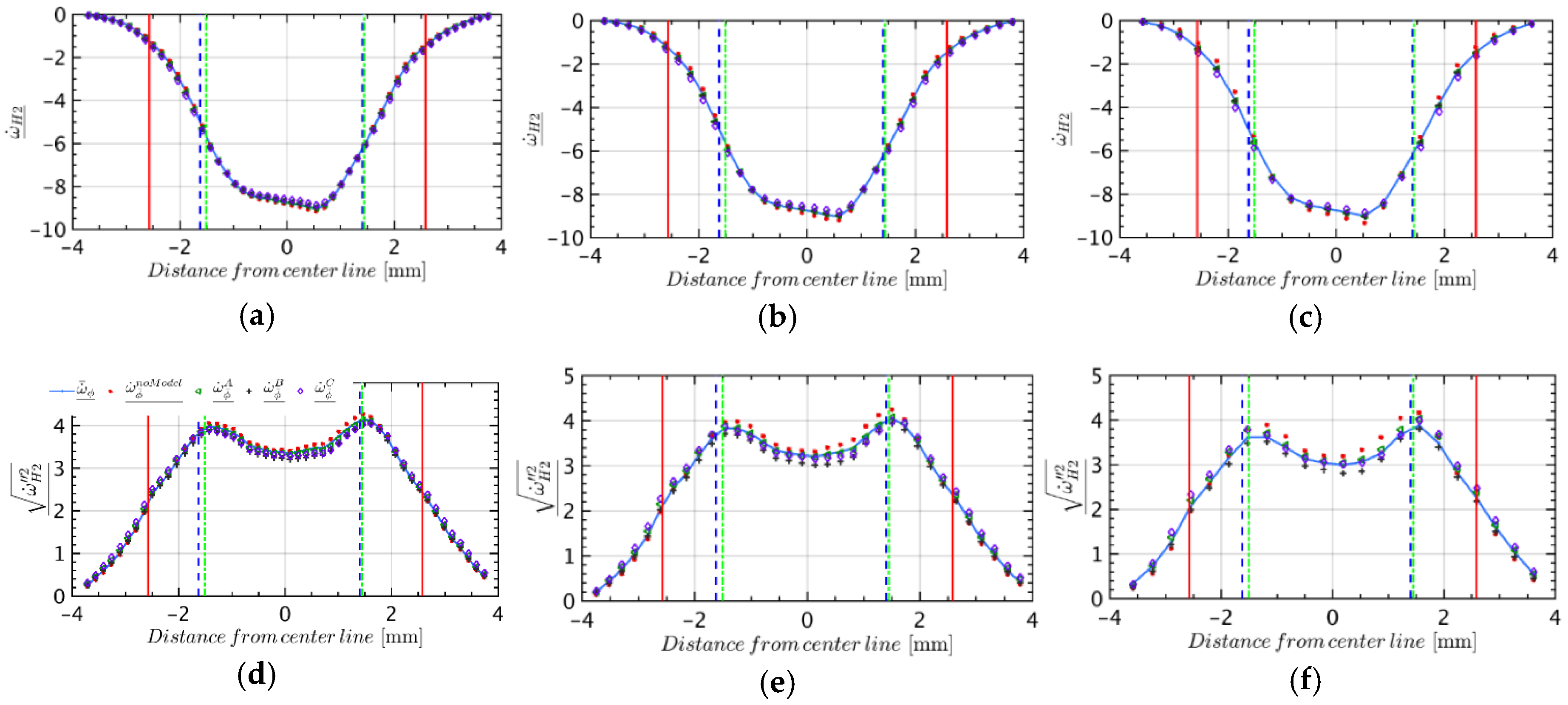
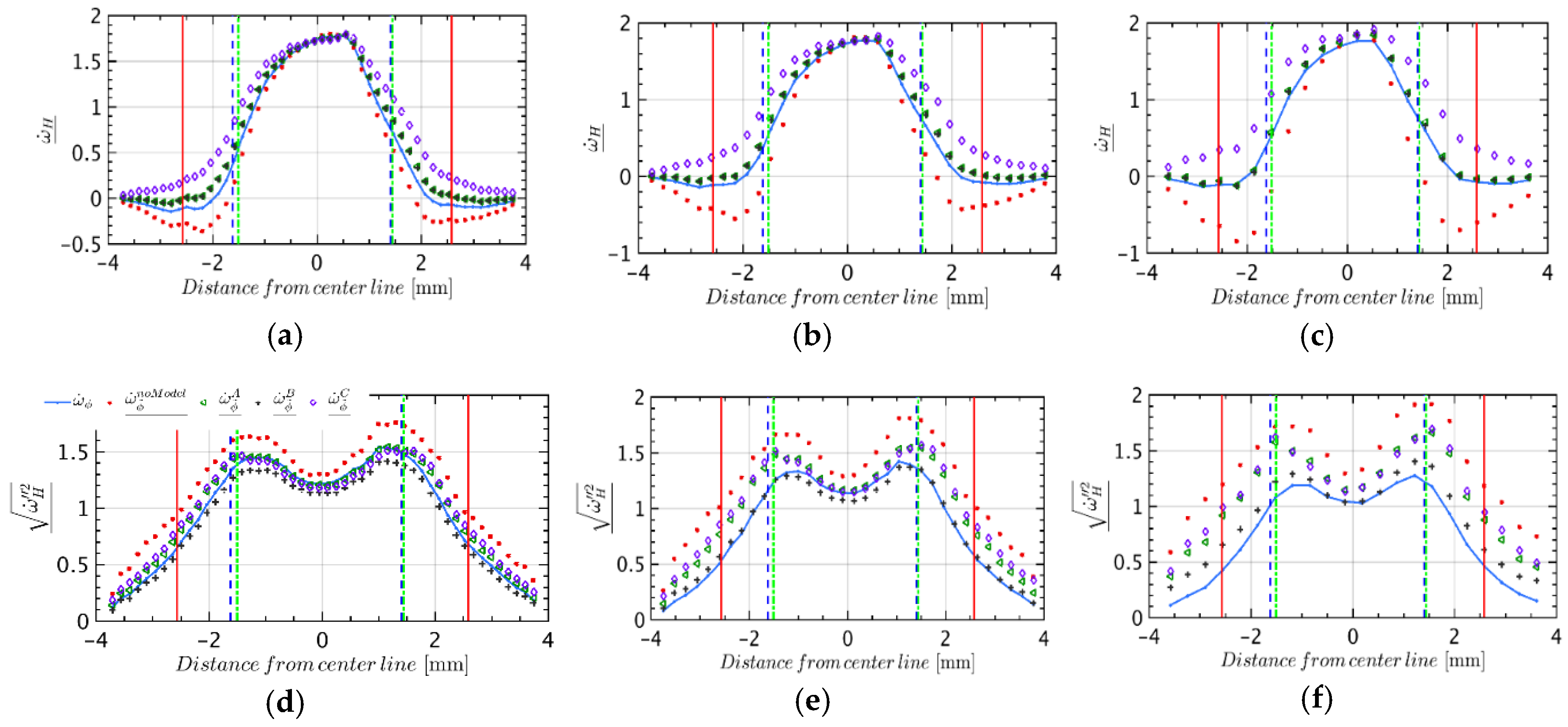
5.4. Heat Release Rates Predictions in Re-Ignition Time

In Figure 10, the filtered heat release rates are depicted. It is observed that, using $\Delta /{\Delta }_{\mathrm{DNS}}=8$, the “no model” approach can predict mean filtered heat release rate with a good accuracy compared to the filtered DNS data. The RMS shown in Figure 10d is a bit higher in the outer flame region which can be corrected by using SS Models A and B. It should be noted that the flame re-ignites from the center of the jet (regions between two vertical green lines). This is evident in high heat release rates in this region. Increasing the filter width increases the error of the “no model” approach (compare Figure 10b,c with Figure 10a). However, SS Models A and B correctly predict the mean filtered heat release rates. In RMS, discrepancies exist compared to the exact filtered DNS data; however, as can be seen in Figure 10d–f, SS models effectively try to decrease the error.

As it can be inferred from the results in the two previous subsections, both SS Models A and B can predict well the mean filtered production/consumption rate of major species and radicals compared to the “no model” approach, in both extinction and re-ignition times. The RMS is captured with a reasonable accuracy by both models. It is found that SS models are able to detect the locations where SGS effects prevail in the flame. As an example, Figure 11 shows the exact SGS or residual scalar field for production/consumption rate of H₂O at time $t=20t_j$ in the xy plane at z = 0. The SGS field is obtained by subtracting ${\dot{\omega }}_{{\mathrm{H}}_2\mathrm{O}}({\overline{\mathbf{\phi }}}^f)$ from ${\overline{\dot{\omega }}}_{{\mathrm{H}}_2\mathrm{O}}^A(\mathbf{\phi })$ where $\Delta /{\Delta }_{\mathrm{DNS}}=12$ is used as the filter width. The performance of SS Model A is assessed by comparing the exact SGS field with ${ℒ}_{{\dot{\omega }}^A}$. Note that ${ℒ}_{{\dot{\omega }}^A}$ is the residual field predicted by Model A and is defined in Equation (7). In Figure 11, it is evident that the SGS structures are captured. The locations of the predicted peak residual field (Figure 11b) are in agreement with the exact residual field (Figure 11a).

6. Conclusions

In the present paper, finite-rate SGS scale similarity combustion models have been used to calculate the filtered combustion and heat release rates of a non-premixed jet flame exhibiting high level of local extinction and re-ignition. Thereby, the performance of three SS type combustion models for LES have been evaluated by means of an a priori assessment using numerical experiment from DNS database of a temporally evolving syngas jet flame [30]. Two SS models, namely the SSRRRM [11], called Model A, and the SSFRRM [11], called Model B, were considered, together with a third model, called Model C, which was derived following the Germano’s/Liu’s approach [25,51]. To summarize, the following conclusions could be drawn:

(1) When looking at mean profiles, it is found that, regardless of the filter width ($\Delta$) applied and the flame regime, Models A and B predicts similar results with good accuracy for both major and minor species. On the contrary, the predictions of Model C for major species have larger errors, especially when using large $\Delta$. Moreover, for radicals, Model C fails to predict the correct mean (see Figure 4 and Figure 8). The failure of Model C is also in line with observations reported in [51], where the Model C performance was found to be very sensitive to the filter width. For small $\Delta$, the incurred error of Model C is higher than using no SGS model. However, by increasing $\Delta$, the error becomes less than the so-called “quasi laminar” or “no model” approach.

(2) In terms of RMS and local errors, Model A performs better than Model B, with smaller local errors for major species such as CO, H₂, CO₂ and H₂O. However, for radicals, the performances of Model B are locally better.

(3) It is found that SS models are able to detect the locations where SGS effects prevail in the flame. This is the advantage of SS models which can accurately detect the locations where SGS effects are high and a model for residual field is needed. The differences in predicting mean and RMS of filtered combustion and heat release rates among the adopted models result from the way that they compute the residual field at the same detected locations. In the current study, it is found that the SS type models which are derived according to “double filtering” approach of Bardina et al. [23] (i.e., Models A and B) have the ability to predict mean profiles with good accuracy at the instant of extinction and re-ignition of the flame. The good agreement is observed even when large filter widths are applied.

The coefficient of similarity in Models A and B (i.e., $C_A^{\overline{\Delta }}$ and $C_B^{\overline{\Delta }}$ in Equations (4) and (6), respectively) were set equal to one in the present study. The effect of modifying this coefficient was not studied since the main focus was the assessment of capability of standard SS models. This analysis is currently in progress.

References

1. Poinsot, T.; Veynante, D. Theoretical and Numerical Combustion, 2nd ed.; Edwards: Queensland, Australia, 2005; ISBN 1-930217-10-2. [Google Scholar]
2. Janicka, J.; Sadiki, A. Large eddy simulation of turbulent combustion systems. Proc. Combust. Inst. 2005, 30, 537–547. [Google Scholar] [CrossRef]
3. Pitsch, H. Large-Eddy Simulation of Turbulent Combustion. Annu. Rev. Fluid Mech. 2006, 38, 453–482. [Google Scholar] [CrossRef]
4. Colin, O.; Ducros, F.; Veynante, D.; Poinsot, T. A thickened flame model for large eddy simulations of turbulent premixed combustion. Phys. Fluids 2000, 12, 1843–1863. [Google Scholar] [CrossRef]
5. Charlette, F.; Meneveau, C.; Veynante, D. A power-law flame wrinkling model for LES of premixed turbulent combustion Part II: Dynamic formulation. Combust. Flame 2002, 131, 181–197. [Google Scholar] [CrossRef]
6. Pope, S.B. PDF methods for turbulent reactive flows. Prog. Energy Combust. Sci. 1985, 11, 119–192. [Google Scholar] [CrossRef]
7. Haworth, D.C. Progress in probability density function methods for turbulent reacting flows. Prog. Energy Combust. Sci. 2010, 36, 168–259. [Google Scholar] [CrossRef]
8. Ertesvåg, I.S.; Magnussen, B.F. The Eddy Dissipation Turbulence Energy Cascade Model. Combust. Sci. Technol. 2000, 159, 213–235. [Google Scholar] [CrossRef]
9. Sabelnikov, V.; Fureby, C. LES combustion modeling for high Re flames using a multi-phase analogy. Combust. Flame 2013, 160, 83–96. [Google Scholar] [CrossRef]
10. Golovitchev, V.I.; Chomiak, J. Numerical Modeling of High-Temperature Air Flameless Combustion. In Proceedings of the 4th International Symposium on High Temperature Air Combustion and Gasification, Rome, Italy, 27–30 November 2001. [Google Scholar]
11. DesJardin, P.E.; Frankel, S.H. Large eddy simulation of a nonpremixed reacting jet: Application and assessment of subgrid-scale combustion models. Phys. Fluids 1998, 10, 2298–2314. [Google Scholar] [CrossRef]
12. Jaberi, F.A.; James, S. A dynamic similarity model for large eddy simulation of turbulent combustion. Phys. Fluids 1998, 10, 1775–1777. [Google Scholar] [CrossRef]
13. Bösenhofer, M.; Wartha, E.-M.; Jordan, C.; Harasek, M. The Eddy Dissipation Concept—Analysis of Different Fine Structure Treatments for Classical Combustion. Energies 2018, 11, 1902. [Google Scholar] [CrossRef]
14. Li, Z.; Ferrarotti, M.; Cuoci, A.; Parente, A. Finite-rate chemistry modelling of non-conventional combustion regimes using a Partially-Stirred Reactor closure: Combustion model formulation and implementation details. Appl. Energy 2018, 225, 637–655. [Google Scholar] [CrossRef]
15. Li, Z.; Cuoci, A.; Sadiki, A.; Parente, A. Comprehensive numerical study of the Adelaide Jet in Hot-Coflow burner by means of RANS and detailed chemistry. Energy 2017, 139, 555–570. [Google Scholar] [CrossRef]
16. Fedina, E.; Fureby, C.; Bulat, G.; Meier, W. Assessment of Finite Rate Chemistry Large Eddy Simulation Combustion Models. Flow Turbul. Combust. 2017, 99, 385–409. [Google Scholar] [CrossRef] [PubMed] [Green Version]
17. Fureby, C. LES of a multi-burner annular gas turbine combustor. Flow Turbul. Combust. 2010, 84, 543–564. [Google Scholar] [CrossRef]
18. Lysenko, D.A.; Ertesvåg, I.S. Reynolds-Averaged, Scale-Adaptive and Large-Eddy Simulations of Premixed Bluff-Body Combustion Using the Eddy Dissipation Concept. Flow Turbul. Combust. 2018, 100, 721–768. [Google Scholar] [CrossRef]
19. Minotti, A.; Sciubba, E. LES of a Meso combustion chamber with a detailed chemistry model: Comparison between the flamelet and EDC models. Energies 2010, 3, 1943–1959. [Google Scholar] [CrossRef]
20. Garnier, E.; Adams, N.; Sagaut, P. Large Eddy Simulation for Compressible Flows; Springer: Dordrecht, The Netherland, 2009; ISBN 9789048128181. [Google Scholar]
21. Wang, Q.; Ihme, M. Regularized deconvolution method for turbulent combustion modeling. Combust. Flame 2017, 176, 125–142. [Google Scholar] [CrossRef]
22. Domingo, P.; Vervisch, L. DNS and approximate deconvolution as a tool to analyse one-dimensional filtered flame sub-grid scale modelling. Combust. Flame 2017, 177, 109–122. [Google Scholar] [CrossRef]
23. Bardina, J.; Ferziger, J.H.; Reynolds, W.C. Improved subgrid-scale models for large-eddy simulation. In Proceedings of the 13th Fluid and PlasmaDynamics Conference, Snowmass, CO, USA, 14–16 July 1980; p. 1357. [Google Scholar] [CrossRef]
24. Germano, M. A proposal for a redefinition of the turbulent stresses in the filtered Navier–Stokes equations. Phys. Fluids 1986, 29, 2323–2324. [Google Scholar] [CrossRef]
25. Liu, S.; Meneveau, C.; Katz, J. On the properties of similarity sub-grid scale models as deduced from measurements in a turbulent jet. J. Fluid Mech. 1994, 275, 83–119. [Google Scholar] [CrossRef]
26. Sagaut, P. Large Eddy Simulation for Incompressible Flows, 3rd ed.; Springer: Berlin, Germany, 2005; ISBN 3-540-26344-6. [Google Scholar]
27. Potturi, A.; Edwards, J.R. Investigation of Subgrid Closure Models for Finite-Rate Scramjet Combustion. In Proceedings of the 43rd Fluid Dynamics Conference, San Diego, CA, USA, 24–27 June 2013; p. 2461. [Google Scholar]
28. Knikker, R.; Veynante, D.; Meneveau, C. A priori testing of a similarity model for large eddy simulations of turbulent premixed combustion. Proc. Combust. Inst. 2002, 29, 2105–2111. [Google Scholar] [CrossRef]
29. Knikker, R.; Veynante, D.; Meneveau, C. A dynamic flame surface density model for large eddy simulation of turbulent premixed combustion. Phys. Fluids 2004, 16, L91–L94. [Google Scholar] [CrossRef]
30. Hawkes, E.R.; Sankaran, R.; Sutherland, J.C.; Chen, J.H. Scalar mixing in direct numerical simulations of temporally evolving plane jet flames with skeletal CO/H2 kinetics. Proc. Combust. Inst. 2007, 31, 1633–1640. [Google Scholar] [CrossRef]
31. Pope, S.B. A model for turbulent mixing based on shadow-position conditioning. Phys. Fluids 2013, 25. [Google Scholar] [CrossRef]
32. Yang, Y.; Wang, H.; Pope, S.B.; Chen, J.H. Large-eddy simulation/probability density function modeling of a non-premixed CO/H2 temporally evolving jet flame. Proc. Combust. Inst. 2013, 34, 1241–1249. [Google Scholar] [CrossRef]
33. Sen, B.A.; Hawkes, E.R.; Menon, S. Large eddy simulation of extinction and reignition with artificial neural networks based chemical kinetics. Combust. Flame 2010, 157, 566–578. [Google Scholar] [CrossRef]
34. Vo, S.; Stein, O.T.; Kronenburg, A.; Cleary, M.J. Assessment of mixing time scales for a sparse particle method. Combust. Flame 2017, 179, 280–299. [Google Scholar] [CrossRef]
35. Scholtissek, A.; Dietzsch, F.; Gauding, M.; Hasse, C. In-situ tracking of mixture fraction gradient trajectories and unsteady flamelet analysis in turbulent non-premixed combustion. Combust. Flame 2017, 175, 243–258. [Google Scholar] [CrossRef]
36. Punati, N.; Sutherland, J.C.; Kerstein, A.R.; Hawkes, E.R.; Chen, J.H. An evaluation of the one-dimensional turbulence model: Comparison with direct numerical simulations of CO/H2 jets with extinction and reignition. Proc. Combust. Inst. 2011, 33, 1515–1522. [Google Scholar] [CrossRef]
37. Vo, S.; Kronenburg, A.; Stein, O.T.; Cleary, M.J. MMC-LES of a syngas mixing layer using an anisotropic mixing time scale model. Combust. Flame 2018, 189, 311–314. [Google Scholar] [CrossRef]
38. Trisjono, P.; Pitsch, H. Systematic Analysis Strategies for the Development of Combustion Models from DNS: A Review. Flow Turbul. Combust. 2015, 95, 231–259. [Google Scholar] [CrossRef]
39. Argyropoulos, C.D.; Markatos, N.C. Recent advances on the numerical modelling of turbulent flows. Appl. Math. Model. 2015, 39, 693–732. [Google Scholar] [CrossRef]
40. Lapointe, S.; Blanquart, G. A priori filtered chemical source term modeling for LES of high Karlovitz number premixed flames. Combust. Flame 2017, 176, 500–510. [Google Scholar] [CrossRef]
41. Ihme, M.; Pitsch, H. Prediction of extinction and reignition in nonpremixed turbulent flames using a flamelet/progress variable model. 1. A priori study and presumed PDF closure. Combust. Flame 2008, 155, 70–89. [Google Scholar] [CrossRef]
42. Ameen, M.M.; Abraham, J. A priori evaluation of subgrid-scale combustion models for diesel engine applications. Fuel 2015, 153, 612–619. [Google Scholar] [CrossRef]
43. Allauddin, U.; Klein, M.; Pfitzner, M.; Chakraborty, N. A priori and a posteriori analyses of algebraic flame surface density modeling in the context of Large Eddy Simulation of turbulent premixed combustion. Numer. Heat Transf. Part A: Appl. 2017, 71, 153–171. [Google Scholar] [CrossRef]
44. Lignell, D.; Hewson, J.C.; Chen, J. a priori analysis of conditional moment closure modeling of a temporal ethylene jet flame with soot formation using direct numerical simulation. Proc. Combust. Inst. 2009, 32, 1491–1498. [Google Scholar] [CrossRef]
45. da Silva, C.B.; Pereira, J.C.F. Analysis of the gradient-diffusion hypothesis in large-eddy simulations based on transport equations. Phys. Fluids 2007, 19. [Google Scholar] [CrossRef]
46. Cuoci, A.; Frassoldati, A.; Faravelli, T.; Ranzi, E. OpenSMOKE++: An object-oriented framework for the numerical modeling of reactive systems with detailed kinetic mechanisms. Comput. Phys. Commun. 2015, 192, 237–264. [Google Scholar] [CrossRef]
47. Zang, Y.; Street, R.L.; Koseff, J.R. A dynamic mixed subgrid-scale Model and its application to turbulent recirculating flows. Phys. Fluids A: Fluid Dyn. 1993, 5, 3186–3196. [Google Scholar] [CrossRef]
48. Gauding, M.; Dietzsch, F.; Goebbert, J.H.; Thévenin, D.; Abdelsamie, A.; Hasse, C. Dissipation element analysis of a turbulent non-premixed jet flame. Phys. Fluids 2017, 29. [Google Scholar] [CrossRef]
49. Pantano, C. Direct simulation of non-premixed flame extinction in a methane–air jet with reduced chemistry. J. Fluid Mech. 2004, 514, 231–270. [Google Scholar] [CrossRef] [Green Version]
50. Pope, S.B. Turbulent Flows, 1st ed.; Cambridge University Press: Cambridge, UK, 2000; ISBN 978-0-521-59886-6. [Google Scholar]
51. Germano, M.; Maffio, A.; Sello, S.; Mariotti, G. On the extension of the dynamic modelling procedure to turbulent reacting flows. In Direct and Large-Eddy Simulation II; Springer: Dordrecht, The Netherland, 1997; pp. 291–300. [Google Scholar]
Figure 1. (a) The schematic of the temporal jet direct numerical simulation (DNS) case, including the contours of heat release rate (colored from black to white) and the mass fraction of OH radical (colored from blue to red) at the maximum extinction time ( t = 20 t j ). Local extinction events on the shear layers are observed with low OH mass fraction and the corresponding low heat release rate; (b) favre averaged mixture fraction ( Z _ f ) in the whole simulation time colored by Favre averaged temperature. The vertical red lines are the time instants analyzed in the current study; and (c) normalized energy spectrum on the center plane (black line) and −5/3 scaling law shown by dashed red line; κ is the wave number, η _ f , Favre averaged Kolmogorov length scale and ε _ f Favre averaged turbulent dissipation rate.
Energies 11 02464 g001
Figure 2. (a) Locations of the cutoff filter with the corresponding filter widths on log-log plot of compensated energy spectrum computed on the central plane; and (b) fraction of the Favre averaged resolved TKE using different filter widths at t = 20 t j .
Energies 11 02464 g002
Figure 3. Production/consumption rate of H2 with units (kg/(m3s)), (-) filtered DNS, () “no model”, () SS Model A, (+) SS Model B, (◇) SS Model C: (ac) Mean; and (df) root mean square (RMS). Different filter widths are applied: (a,d) ∆/∆DNS = 8; (b,e) ∆/∆DNS = 12; and (c,f) ∆/∆DNS = 18. The data are extracted at t = 20 t j . vertical dashed-blue lines: planes of maximum mean turbulent kinetic energy (TKE); vertical dot-dashed green lines: planes of mean stoichiometric mixture fraction; and vertical red lines: planes of maximum mean temperature fluctuations.
Energies 11 02464 g003
Figure 4. Production/consumption rate of H with units (kg/(m3s)): (ac) Mean; and (df) RMS. Different filter widths are applied: (a,d) ∆/∆DNS = 8; (b,e) ∆/∆DNS = 12; and (c,f) ∆/∆DNS = 18. The data are extracted at t = 20 t j . Vertical lines are the same as in Figure 3.
Energies 11 02464 g004
Figure 5. Cumulative local errors incurred using different models in prediction of different species net formation rates: (ac) logarithm of errors for all models; and (df) the errors divided by the “no model” approach error. Different filter widths are applied: (a,d) ∆/∆DNS = 8; (b,e) ∆/∆DNS = 12; and (c,f) ∆/∆DNS = 18. The data are extracted at t = 20 t j .
Energies 11 02464 g005
Figure 6. Heat release rate with units (kg/(ms3)): (ac) Mean; and (df) RMS. Different filter widths are applied: (a,d) ∆/∆DNS = 8; (b,e) ∆/∆DNS = 12; and (c,f) ∆/∆DNS = 18. The data are extracted at t = 20 t j . Vertical lines are the same as in Figure 3.
Energies 11 02464 g006
Figure 7. Production/consumption rate of H2 with units (kg/(m3s)): (ac) Mean; and (df) RMS. Different filter widths are applied: (a,d) ∆/∆DNS = 8; (b,e) ∆/∆DNS = 12; and (c,f) ∆/∆DNS = 18. The data are extracted at t = 35 t j . Vertical lines are the same as in Figure 3.
Energies 11 02464 g007
Figure 8. Production/consumption rate of H with units (kg/(m3s)): (ac) Mean; and (df) RMS. Different filter widths are applied: (a,d) ∆/∆DNS = 8; (b,e) ∆/∆DNS = 12; and (c,f) ∆/∆DNS = 18. The data are extracted at t = 35 t j . Vertical lines are the same as in Figure 3.
Energies 11 02464 g008
Figure 9. Cumulative local errors incurred using different models in prediction of different species net formation rates: (ac) logarithm of errors for all models; and (df) the errors are divided by the “no model” approach error. Different filter widths are applied: (a,d) ∆/∆DNS = 8; (b,e) ∆/∆DNS = 12; and (c,f) ∆/∆DNS = 18. The data are extracted at t = 35 t j .
Energies 11 02464 g009
Figure 10. Heat release rate with units (kg/(ms3)): (ac) Mean; and (df) RMS. Different filter widths are applied: (a,d) ∆/∆DNS = 8; (b,e) ∆/∆DNS = 12; and (c,f) ∆/∆DNS =18. The data are extracted at t = 35 t j . Vertical lines are the same as in Figure 3.
Energies 11 02464 g010
Figure 11. Residual ω ˙ H 2 O with units (kg/(m3s)) when DNS is filtered by using Δ / Δ DNS = 12 at t = 20 t j : (a) Exact; and (b) Predicted by Model A. Cut-off plane is the central xy plane.
Energies 11 02464 g011