Linearized Stochastic Scheduling of Interconnected Energy Hubs Considering Integrated Demand Response and Wind Uncertainty

1
College of Electrical Engineering, Zhejiang University, Hangzhou 310027, China
2
Electrical and Computer Engineering Department, Illinois Institute of Technology, Chicago, IL 60616, USA
*
Authors to whom correspondence should be addressed.
Energies 2018, 11(9), 2448; https://doi.org/10.3390/en11092448
Submission received: 4 September 2018
/
Revised: 10 September 2018
/
Accepted: 12 September 2018
/
Published: 14 September 2018
(This article belongs to the Special Issue Applied Energy System Modeling 2018)
Abstract
:In the context of the Energy Internet, customers are supplied by energy hubs (EH), while the EHs are interconnected through an upper-level transmission system. In this paper, a stochastic scheduling model is proposed for the interconnected EHs considering integrated demand response (DR) and wind variation. The whole integrated energy system (IES) is linearly modeled for the first time. The output-input relationship within the energy hub is denoted as a linearized matrix, while the upper-level power and natural gas transmission systems are analyzed through piecewise linearization method. A novel sequential linearization method is further proposed to balance computational efficiency and approximation accuracy. Integrated demand response is introduced to smooth out demand curve, considering both internal DR achieved by the optimal energy conversion strategy within energy hubs, and external DR achieved by demand adjustment on the customer’s side. Distributed energy storage like natural gas and heat storage are considered to provide buffer for system operation. The proposed stochastic model is solved by scenario-based optimization with a backward scenario reduction strategy. Numerical tests on a three-hub and seventeen-hub interconnected system that validates the effectiveness of the proposed scheduling model and solution methodology.
1. Introduction
Energy is the lifeblood of society development. Driven by lower gas price and environmental policy, natural gas consumption of the world’s total energy resource is predicted to be 28% by 2030, while the installed capacity of wind power is also rapidly growing [1]. With the progress of “The Third Industrial Revolution”, traditional power system has involved the Energy Internet with the integration of electricity, natural gas, heat, wind, and other forms of energy [2]. Energy Internet plays an important role in improving energy conversion efficiency, enhancing social infrastructure utilization, promoting renewable energy penetration, and guaranteeing energy supply security. The short-term operation of this newborn integrated energy system (IES) becomes a severe challenge. A novel comprehensive model and analysis method are critical to provide the more flexible and sustainable energy supply.
Based on the transmission and distribution level, the structure of the IES can be classified as transportation infrastructure across long distances called energy interconnectors and energy conversion facilities in terminal district called energy hubs (EH) [3]. In terms of multi-energy transmission networks, various studies have been carried out. A detailed and uniform model for integrated electricity-natural gas system (IEGS) was proposed in Reference [4], and the interaction mechanism between both systems was further analyzed in Reference [5]. To achieve better system operation reliability, the resilient IEGS planning strategies against malicious attacks and extreme disasters were proposed in References [6,7], and the secure IEGS operation strategies against wind uncertainty and N-1 criterion were analyzed in References [8,9]. Synergetic operation between these two energy systems was achieved in Reference [10], while the fully decentralized decision among each regional system was achieved in Reference [11] through the alternating direction method of multipliers (ADMM). Second-order cone relaxation was applied in the natural gas system for convexification in Reference [12], but the tightness of relaxation could not be guaranteed. Note that the nonlinear terms in natural gas flow leads to computational complexity, a linearized model based on incremental formulation was proposed in References [13,14]. However, the main drawback of the current linearization method is the model accuracy that highly relies on the number of piecewise segments, so approximation accuracy, and solution efficiency cannot be achieved simultaneously.
Energy hub like large campus or industrial zone can be considered as an interface between multiple energy inputs and outputs. They obtain energy source from upper-level network and distribute energy to end-users. Variable kinds of energy conversion equipment like solar power plants and electric vehicles (EV) were introduced into an energy hub for energy cascade utilization [15], and the multi-period framework for electric vehicle dispatch was proposed in Reference [16] considering that a driver is satisfactory. The benefits of electricity storage in a distribution network was discussed in Reference [17]. These conversion components expand the content of EH. These input/output ports are related through a coupling matrix, which is usually nonlinear [3]. Based on it, the optimal energy flow of single EH was proposed in Reference [18]. The design strategy of EH was discussed in Reference [19] and the effectiveness of EH in promoting wind penetration was validated. The nonlinearity of EH modeling led to solution inefficiency. While fixed dispatch factor was applied for EH to eliminate nonlinear terms in References [20,21], global optimality was sacrificed. An up-to-date efficient linear model for EH was first proposed in References [22,23], which described the input/output relationship through augmented linearized coupling matrix. The corresponding linearized EH model could be easily solved by LP solvers. In terms of interconnected EHs, its optimal energy flow model was first proposed in Reference [24] by considering transmission network and terminal EH as a comprehensive infrastructure. The decomposed operation model for interconnected EHs was discussed in References [25,26], which decomposed the multi-carrier optimal power flow problem into a traditional separate one. It should be mentioned that due to the inherent nonlinearity of transmission network and EH, the current model of the whole interconnected EHs is still nonlinear and complex, a nonlinear solver like Interior Point OPTimizer (IPOPT) and the Genetic Algorithm were applied with a low solution speed [24,25,26].
Demand response (DR) has attracted attention due to its great potential and benefit system operation efficiency, flexibility, and reliability. Energy demand can also be adjusted by end-users according to price signal, and price-elastic electricity demand was discussed in Reference [27]. Time-shifting demand response was incorporated in day-ahead scheduling of power systems in Reference [28], with which, users could shift electricity demand between peak and off-peak period as per the operator command. This kind of demand response was further discussed in IEGS for managing the variability of renewable energy in Reference [29]. The external power and heat demand response was discussed in Reference [30], and DR between power and natural gas based on energy conversion was discussed in Reference [31]. Interruptible load (IL) is another kind of demand response program that is incentive-based, so customers can reduce their load when needed [32]. The above demand response programs can be regarded as external DR since they are implemented by end-users. However, in an Energy Internet environment, energy demands become more flexible since EH makes it possible for energy users to switch the source of consumed energy. It was pointed out in Reference [33] that the efficiency of IES is affected by two factors, one is the energy conversion strategy within each EH, as internal factor, and the other is the traditional demand-side response of end-users as an external factor. Therefore, a traditional DR program gradually develops to integrated DR (IDR). The basic concept of which was first systematically given in this Reference, but the detail interaction and mechanism between internal and external DR needs to be further investigated.
The operation of IES is confronted with various uncertain factors, e.g., wind power fluctuation and equipment random failure. How to achieve higher system reliability against these uncertainties requires an accurate description of stochastic procedure. Various stochastic models have been discussed separately on a transmission network or terminal EH. In terms of a transmission network, stochastic scheduling based on scenario-based, chance-constrained, interval, and robust optimization has been discussed in References [28,29] and References [34,35]. Compared to other methods, scenario-based approach provides more stable and accurate results, which is also easily implemented and has been widely applied [36]. In terms of terminal EH, researches need to handle the uncertainties in energy demand and renewable generation have been done in Reference [19] and References [37,38]. However, the stochastic model of interconnected EHs considering the interaction between the two networks is still a new topic.
While these previous references have greatly promoted Energy Internet, they still have the following limitations. Firstly, current works mainly focus on the scheduling of a transmission system or terminal EH separately. While some works have studied the operation of interconnected EHs, the coordinated model is still nonlinear and complex. Secondly, the computational performance of current one-time linearization method can be improved. Too many or too few piecewise segments can lead to either solution inefficiency or approximation inaccuracy. Thirdly, the mechanism of integrated demand response under Energy Internet environments needs to be further investigation. Besides external DR, internal DR should be included to consider the freedom of EH operation. Finally, stochastic analysis for the whole interconnected EHs is still in progress and the benefits of integrated DR and distributed storage in promoting wind penetration are not discussed yet.
In contrast to these studies, this paper aims at presenting a linearized stochastic model for interconnected EH operation considering integrated demand response and wind uncertainty. A new solution methodology is also proposed for better computational performance. The main contributions of this paper are fourfold:
- (1)
- A linearized model for the whole interconnected EHs considering both transmission network and terminal EHs is proposed. In this model, operation constraints of multi-energy transmission system are piecewise linearized, while terminal EH is modelled through a linearized coupling matrix.
- (2)
- A novel sequential linearization method is further proposed to solve the primal mixed integer linear programming (MILP) problem. Compared to the traditional one-time linearization method, the proposed sequential method can achieve a win-win performance in both solution time and approximation accuracy.
- (3)
- Integrated demand response is detailly modeled, which includes internal and external DR. Internal DR is achieved by the optimal energy conversion strategy within the energy hub, while the external DR is achieved by time-shifting and interruptible DR programs on an end-user’s side.
- (4)
- Stochastic scheduling model for interconnected energy hubs considering wind uncertainty, integrated DR and distributed storage utility is systematically proposed. The benefits of integrated demand response in enhancing the system economy and operation security are tested.
The rest of this paper is organized as follows: The proposed stochastic scheduling model for interconnected EHs with transmission system constraints is formulated in Section 2. The mechanism of integrated demand response is detailly presented in Section 3. Section 4 illustrates the solution methodology. In Section 5, numerical results tested on three-hub and seventeen-hub interconnected system are demonstrated. Section 6 concludes the paper.
2. Formulation of Interconnected Energy Hubs
2.1. Introduction of Interconnected EHs
With the development of Energy Internet strategy, multiple energy carriers, including electricity, natural gas, heat, and other forms of energy, are strongly integrated. This revolution of traditional social pattern helps in promoting the incorporation of renewable energy and the reliability of energy supply. This newborn social pattern can be regarded as a system with interconnected energy hubs.
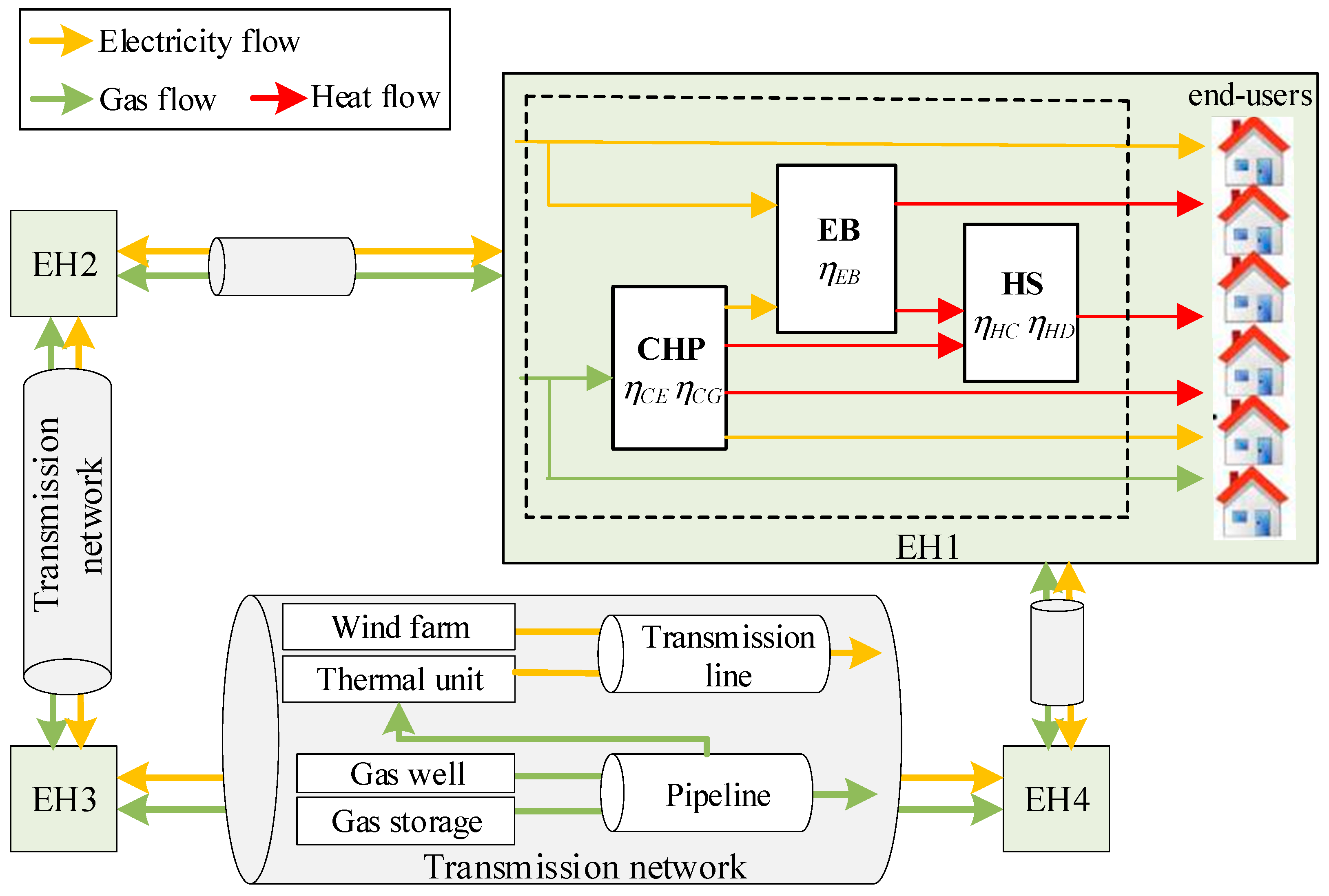
Figure 1 shows the typical topology of interconnected energy hubs. Four EHs are connected through upper-layer transmission system including electricity and natural gas networks [24,25,26]. In the electricity system, generators including thermal units and wind farms can provide electricity to terminal EH as energy inputs. As for the natural gas system, gas wells, and large gas storage facilities can provide natural gas to terminal EHs. Within each EH, energy inputs are converted into multiple outputs through different conversion equipment like combined heat power plant (CHP), electric boiler (EB), and heat storage (HS). Thanks to the freedom of EH operation, energy hub can choose different energy conversion strategy and realize fully utilization of resource. These types of energy are then distributed to end-users to satisfy their daily requirement.
2.2. Objective Function
Our model aims at satisfying end-users’ energy demand while considering the operation of a transmission system, terminal EH and integrated demand response strategy. Standing on a system operators’ perspective, the objective of this paper is to minimize the expected operation cost of interconnected EHs across all wind power scenarios, including the costs of DR program, unit commitments, hourly generation of coal-fired units, hourly production of natural gas wells, and the punishment of wind curtailment and load shedding. Since all these terms can be linearly represented, the objective function is linear and convex.
The energy system with interconnected EHs consists of an upper-level system as the transmission component and a lower-level EH as the energy conversion. The objective is subject to the following constraints for each scenario.
2.3. Transmission System Constraints of Interconnected EHs
These transmission constraints aim at guaranteeing the security and feasibility of multi-energy system operation, so electricity and natural gas can be transmitted to terminal EHs as inputs. The constraints of interconnected EHs in the upper-layer transmission system includes those of unit commitments, electricity network, natural gas network, and distributed natural gas storage.
(1) Unit commitment constraints
For thermal generators, their unit commitments are restrained by (2)–(9). Constraint (2) limits the generation capability of thermal units, while constraint (3) and (4) limit the upward/downward ramping capability. The linear cost curve of coal-fired unit is given as constraint (5), while constraint (6) enforces the generation limit on each segment. The economic cost and gas consumption of thermal units through startup/shutdown are calculated by constraint (7) and constraint (8). Constraint (9) represents the minimum ON/OFF time limits for thermal units. It should be noted that the bilinear terms in constraints (3)–(9) can be easily eliminated through auxiliary variables, so unit commitment constraints are totally linear.
(2) Electricity network constraints
Electricity network are restrained by constraints (10)–(13). Constraint (10) states that electricity at each bus should be balanced. Constraint (11) calculates the power flow on the transmission line by the DC-method, and the limited transmission capacity should be lower than its maximum bound. Nodal phase angle is restricted within its feasible region by constraint (12). Constraint (13) represents that redundant wind power can be curtailed when necessary. Electricity demands in transmission system serve as electricity inputs in terminal EHs.
(3) Natural gas network constraints
Natural gas network is restrained by constraints (14)–(20). Constraints (14) and (15) represent the limits on gas well production and nodal pressure. Natural gas flow is modeled by the nonlinear Weymouth function as constraint (16), which is determined by the incremental pressure between two end nodes of pipeline, and is the average gas flow of pipeline mn. Constraint (17) represents the limit on nodal gas balance. Nodal natural gas demand is calculated by constraint (18), including that of the natural gas-fired units (NGUs) and energy hubs. Note that natural gas is measured in volume unit in transmission network and energy unit in terminal EH, the conversion is denoted by . This paper only discusses passive pipelines, so compressors are not considered in the model. Compared to the steady-state model, dynamic characteristic of natural gas flow is described by linepack, which allows the diverse inflow/outflow rate of the same pipeline [13]. Linepack can be considered as proportional to the pipeline average pressure as constraint (19), where the pipeline average pressure is calculated by . Intertemporal constraint of linepack is given in constraint (20).
(4) Distributed storage constraints
Compared to battery storage, natural gas storage with a large capacity like a gas tank is more efficient in IES. Distributed storage utility can serve as alterable energy production or demand when the security of natural gas network is challenged. Constraints (21)–(23) are the operation constraints of natural gas storage, including those of storing/releasing capability and the state of the gas (SOG) limitation. Constraint (23) also denotes the intertemporal constraint of SOG between sequential time periods. To avoid end-of-horizon effects associated with a finite number of scheduling periods, constraint (24) requires that SOG of storage at the end of scheduling window should be set as the initial interval. It should be noted that other storage facilities like battery storage and power-to-gas device can be easily introduced in the proposed model. It should be noted that other storage facilities like large charging stations for EVs and power-to-gas devices can be easily introduced in the proposed model. Factors like a driver’s behavior and a driver’s preference should be considered when EVs are included. These facilities can provide buffer for IES operation and enhance system reliability and economy.
2.4. Coupling Constraint
Since most of the thermal units are non-quick-start units, their ON/OFF status cannot be instantly changed; the unit commitment strategy should be the same for all scenarios. Constraint (25) shows that the decision of unit commitment should be made here-and-now, rather than wait-and-see after wind uncertainty unfolds. However, other decision variables like unit generation and gas well production can be adjusted according to wind variation, as shown above.
In an integrated energy system, electricity, and natural gas network are connected as a coupled infrastructure through NGUs. NGUs serve as an energy producer in electricity system and an energy consumer in natural gas system. Constraint (26) presents the coupled conversion from natural gas input to electricity output through NGUs.
3. Integrated Demand Response
3.1. Overview of Integrated Demand Response
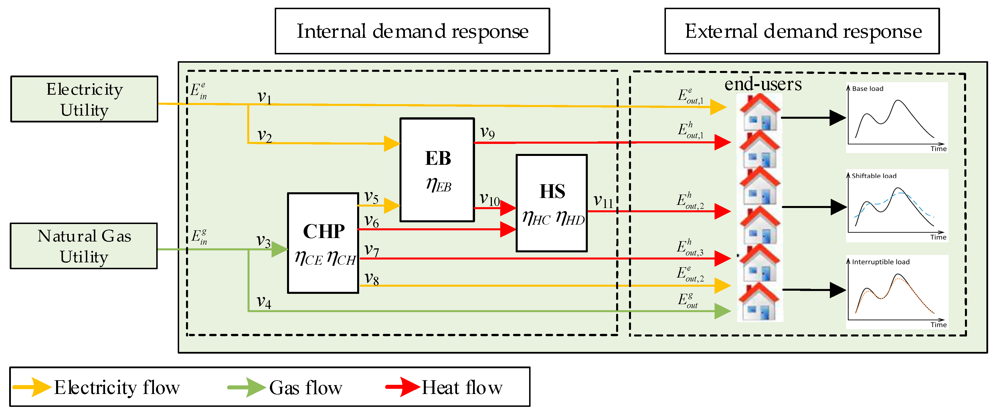
Figure 2 ilustrates the schematic of integrated demand response, inlcuding internal DR and external DR, according to the actural implementer.
Within each energy hub, by integrating electricity, natural gas, heat, and other forms of energy together, it is possible to switch the source of consumed energy flexibly [33]. For example, EH can reduce electricity demand during power system peak, and resort to natural gas sources. Though the optimal energy conversion strategy of EH, even must-run loads can actively participate in DR programs without sacrificing end-users’ comfort. Since this kind of DR is achieved by the freedom of EH inner operation, it is called the internal demand response in this paper.
In terms of the end-users’ side, users can respond to the system through adjusting their energy consumption behaviour. Some demand can flexibly shifted to other time periods by end-users, and some demand can be interrupted with a relatively low compensation. Since these responsive energy demands are based on an outer signal like system command or ecominic incentive and implemented by end-users, they are called external demand responses in this paper.
Note that both internal and external demand response can optimize the inputs of EHs, the introduction of integrated DR and the full exploition of the demand side resource can therefore help in the economy improvement and reliability enhancement of the multi-energy system.
3.2. Internal Demand Response by EH
Figure 2 also illustrates a typical topology of EH, consisting of three-conversion equipment. CHP gets natural gas input from upper-layer transmission system and generate electricity and heat to end-users. Electric boiler converts the electricity provided by a transmission system and CHP into heat. Heat storage servers as a buffer to release or store heat.
EH can be modelled as a coordinated unit with multiple inputs and outputs as constraint (27).
where
Based on the oriented graph of energy flows inside EH like Figure 2, coupling matrix Cr can be denoted as constraint (30) [22]. Each row of coupling matrix Cr represents the relationship among energy flows inside an EH. For example, the first three rows denote the constitution electricity, natural gas and heat output, respectively. The forth row denotes that the input electricity can be either transferred to EB or directly to end-users. The sixth row calculates the change of heat stored in HS with storing and releasing efficiency. This graphics-based method leads to a compact formulation of the energy converters and their connections. In this way, the relationship between inputs and outputs in EH is linearly modelled. Compared to nonlinear matrix with variable dispatch factor, linear model applied in this paper can highly improve solution efficiency while retaining the freedom for EH operation.
Since all rows of input vector except represent energy flow with certain direction, they should be positive. Constraint (31) denotes the storing and releasing capability of heat storage. The intertemporal constraint of stored heat in HS is given as constraint (32), and the capacity limit of stored heat is also provided. Constraint (33) guarantees that the inputs of CHP and EB should be no more than their maximum bounds.
In this paper, we only focus on a typical EH with CHP, EB, and HS. Actually, conversion equipment like electricity storages, electric vehicles, and photovoltaics can also play important roles in EH operation. For example, similar to heat storage, electricity storage can enhance operation reliability through smoothing electricity demand curve. With the graph-based method, the EH can still be easily and linearly modelled with extended input/output vector and coupling matrix when other components are considered.
3.3. External Demand Response on Users’ Side
Demand side nowadys becomes much more active in energy management. For typical end-user, its demand can be categorized into three types, which are base load, shiftable load, and interruptible load. Base load is the part that should be entirely satisfied during operation. However, when system reliablity is in danger during peak hours or contingency, load shedding can be implemented. Shiftable and interruptible load are the parts obligated to time-shifting and interruptible DR, respectively. The energy demand of customers after external demand response can be calculated as constraint (34), where the first term is original energy demand, the second and third terms are the time-shifting DR, the forth term is the interrpuible DR, and the last represents the load shedding in emergency. Due to the extremely high punishment fee, demand tends not to be shed unless necessary.
(1) Time-shifting DR
Shiftable load represents the demand, which can be flexibly shifted from peak to off-peak periods as per the system operator’s command. Since this kind of DR has almost no effect on customer satisfaction, no additional dispatch fee is needed [27,29]. Constraints (35)–(37) demonstrate the constraints of time-shifting DR in various forms of energy, including electricity, natural gas and heat. Constraints (35) and (36) restrict the amount of demand that can be shifted in or out of interval t, respectively. Constraint (37) denotes that the daily demand of the same form of energy stays unchanged after time-shifting DR program.
(2) Interruptible DR
Interruptible load represents the demand that can provide demand relief when necessary. End-users should make contracts with system operators to reserve interruptible demand resource. Constraint (38) calculates the cost of interruptible DR, including the capacity fee and energy fee compensated to end-users [32]. Constraint (39) represents the maximum amount of interruptible load, which is decided before day-ahead or even a longer time period.
Note that our proposed integrated DR model is facing to future integrated energy system, which is much more intelligent and advanced than is present. Three important issues should be addressed to guarantee the implement of proposed DRD program. Firstly, communication between system operators and end-users should be enhanced. Detailed information should be provided to reflect system commands and users’ preference. Secondly, appropriate incentive policy is acquired to motivate the interaction on user’ side. Factors related to users’ response should be further analyzed. Last, but not least, advanced electronic equipment like smart meters should be widely applied to control demand response accurately.
4. Solution Methodology
4.1. Scenario Reduction
Scenario-based optimization is a typical method to solve the stochastic model. In this paper, backward scenario reduction is applied to preserve N scenarios out of M wind power scenarios [39]. The input stochastic data includes the hourly wind energy forecast and error with a normal distribution. The original M scenarios are thus generated by sampling.
Details of backward scenario reduction is given as follows:
- Step 1.1:
- Initialize the probability of all the scenarios as . Set the number of current scenarios .
- Step 1.2:
- Compute the Kantorovich distances of all the scenario pairs as:
- Step 1.3:
- For each wind power scenario si, find the minimum distance and multiply it with the probability of scenario si by
- Step 1.4:
- Remove scenario si with the minimum PKD and accumulate its probability on its closest scenario sj as:
- Step 1.5:
- Update the number of preserved scenarios by , where ni is the number of removed scenarios. Repeat Steps 1.2–1.5 until .
4.2. Sequential Linearization for Better Computational Performance
Due to the quadratic Weymouth function (16) in a natural gas system, the proposed model is nonlinear and inapplicable to efficient optimizer like Gurobi (6.5.0, Gurobi Optimization, Inc., Beaverton, OR, USA). While linearization method is provided in constraints [13,14] to transform the primal nonlinear model into solvable MILP, the approximation accuracy and solution efficiency are mutually exclusive and highly rely on the number of piecewise linear segments. How to balance accuracy and efficiency is an interesting topic.
Noticing that the major challenge of MILP solution is integer variables (piecewise linear segments), a novel sequential linearization method for a natural gas system is proposed in this paper. The key idea is to find the relative rough operational domain of a gas system by initial linearization, and then determine the more accurate domain through further linearization until the approximation accuracy is satisfied.
Details of the proposed sequential linearization method is given as follows:
- Step 2.1:
- Set the whole operational domain as active segments. Set the initial approximation accuracy indexes Af = 1, Ap = 1. Set the satisfied accuracy Afmin, Apmin.
- Step 2.2:
- Set the piecewise segment numbers of natural gas flow kf and nodal pressure kp.
- Step 2.3:
- Based on the current active segments, linearize quadratic terms in constraint (16) through incremental formulation. Gas flow squared can therefore be linearized as constraints (40)–(42), where is the binary for segment l. Similar linearization can be applied to pressure squared .
- Step 2.4:
- Solve the converted MILP model through the linearization of natural gas system in Step 2.3 Find the rough domain of system operation and set new active segments.
- Step 2.5:
- Update approximation accuracy indexes by Af = kf·Af and Ap = kp·Ap, and check if the approximation accuracy is satisfied:Af ≥ Afmin and Ap ≥ Apmin
If yes, the sequential linearization procedure ends. Otherwise, repeat Steps 2.2–2.5 for further linearization.
Through the proposed sequential linearization method, the piecewise procedure is only applied to the selected active segments rather than the whole operational domain, which can greatly reduce the quantity of integer variables (piecewise segments) while guaranteeing the same solution accuracy. Both approximation accuracy and computational efficiency can therefore be achieved.
4.3. Overall Procedure
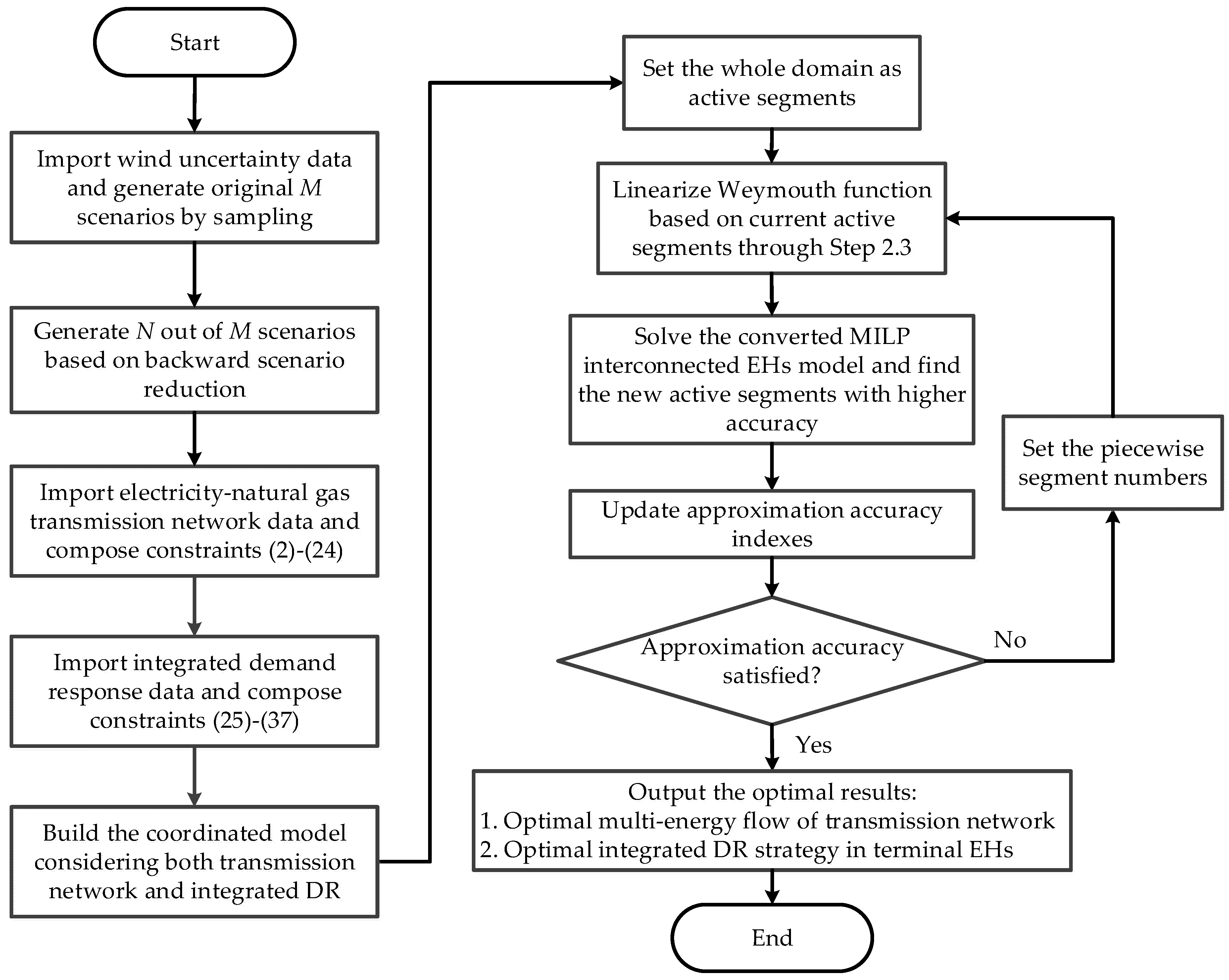
The overall procedure of proposed stochastic model for interconnected EHs is described as Figure 3, which consists of two main parts. One is to build a coordinated stochastic model considering transmission network and integrated demand response. The other is to solve the model by the proposed sequential linearization method.
It should be noted that through the proposed linearization method in Section 4.2, the whole optimization model is converted into MILP, whose compact construction can be described as:
where denotes an m-dimensional vector including continuous variables, denotes an n-dimensional vector including integer variables. , , , and are matrixes or vectors for parameters. MILP is a common optimization model that has a mature and global optimal solution. Since existing solvers like Cplex (https://www.ibm.com/analytics/cplex-optimizer) and Gurobi (http://www.gurobi.com) show high-quality performance in MILP, the convergence of the proposed model and sequential linearization method is perfectly guaranteed, as long as the topology and parameters of the test systems are reasonable.
5. Case Studies and Discussion
In this section, simulation results are tested on three-hub and seventeen-hub interconnected system in day-ahead scheduling window to demonstrate the effectiveness and practicability of the proposed model. Three-hub systems mainly focus on the characteristics of proposed integrated energy system, including energy conversion, distributed storage, integrated demand response, and wind uncertainty. A seventeen-hub system mainly discusses the computational performance of the proposed sequential linearization method. Penalty of load shedding and wind curtailment are set at 1000 $/MWh and 20 $/MWh, respectively. Compensation of IL capacity and energy are set at 1$/MW and 100 $/MWh, respectively. Tests are performed on a PC with Intel Core i7—4790 CPU (4.0 GHz) and 8 Gb of memory. The proposed model is coded in MATLAB 2014 b platform with YALMIP toolbox, and solved by the MILP of Gurobi 6.5.0 toolbox. Parameters of the solvers are set as default. The full system data is available on our provided website, and the source code is available from the authors upon reasonable request.
5.1. Three-Hub Interconnected System
The system is tested in day-ahead scheduling window and its topology is shown as Figure 4. Three EHs are embedded on bus C/node 2, bus D/node 3 and bus E/node 1, respectively. The power transmission system has two natural gas-fired units, one coal-fired unit, one wind farm, and seven transmission lines. Gas transmission system consists of two gas wells, one natural gas storage, and five pipelines. All the system parameters are given in motor.ece.iit.edu/data/ConnectedEH3_stochastic.xlsx.
In this section, three following cases are examined:
- Case I:
- Deterministic scheduling of EHs under forecasting wind power and without integrated demand response.
- Case II:
- Integrated DR is considered in Case I.
- Case III:
- Stochastic scheduling of EHs with variable wind power and integrated DR.
(1) Case I
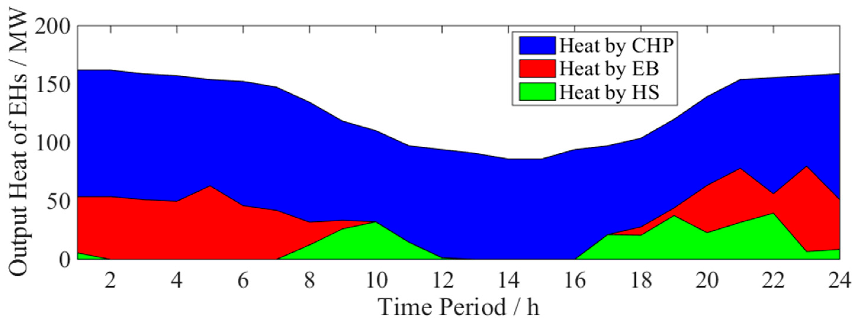
This case aims at analyzing the effectiveness of proposed interconnected EHs model in terms of energy conversion and distributed storages. The integrated DR program is not considered in this case. Perfect wind forecast is obtained from the Belgium market operator’s website [40]. Figure 5 shows the construction of the input and output energy of EHs. In the transmission level, electricity is provided by wind and thermal units, while natural gas is provided by gas wells. These resources are then transmitted to terminal EHs as input energy. Natural gas, thermal power, and wind power account for 56.3%, 30.6%, and 13.1% of the total input energy, respectively. Figure 6 shows the heat demand satisfied by different energy conversion equipment. CHP provides most of heat demand due to its high conversion efficiency, especially during daytime. However, due to the increased heat demand at night, the capacity of CHP is not adequate to satisfy all the heat demand, so other conversion equipment like electric boiler and heat storage function as alternative heat suppliers. In this case study without DR program, 263.56 MW heat demand is inevitably shed at night due to system congestion and inadequate equipment capacity. Infrastructure construction is needed for reliable system operation. In terms of electricity demand on users’ side, the majority is directly provided by input electricity without conversion loss, the rest is the electricity CHP generates when producing heat. The portion of electricity demand supplied by CHP stays unchanged since EH is unable to adjust its operation status when internal DR is not considered.
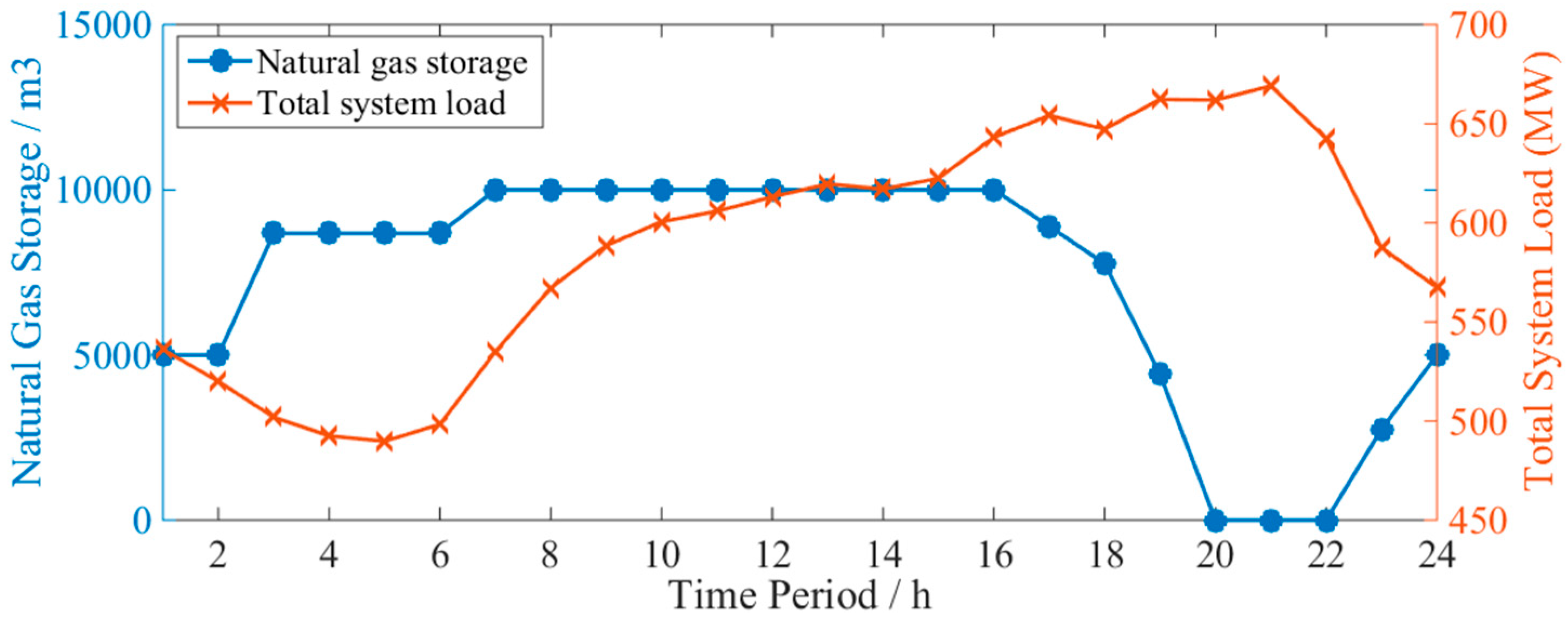
Since natural gas system is congested during peak hours in this case, more electricity tends to be generated by non-NGUs since some NGUs cannot get adequate gas sources in transmission system. In terms of terminal EH, EH refers to electricity for energy conversion due to inadequate natural gas input. In this situation, distributed gas storage is a good cushion for system operation, which can serve as a gas supplier or a gas demand depending on load curve. The amount of natural gas stored in storage and total system load is shown in Figure 7. It is obvious that stored gas has different peak and valley characteristics as system load. Since system load is in its valley in the early morning, the system has redundant transmission capacity and natural gas storage is filled during this period. The SOG of storage reaches to its peak at seven h and keeps constant until 16 h. Since then, distributed storage releases natural gas corresponding to the subsequent peak load. Storage is filled again and prepare for next-day operation. $26,170 is saved with the introduction of natural gas storage, and less-load is curtailed since storage benefits in switching gas demand from peak to off-peak hours.
(2) Case II
In this part, four different DR strategies (without DR, internal DR only, external DR only and with integrated DR) are compared to validate the advantage of demand response in interconnected EHs. Solution results are given in Table 1. Without DR program in Case I, the total operation cost is the highest. Congestion in upper-level transmission network prevents the efficient transmission of energy, a total load of 423.12 MW is inevitably shed between 16 h and 22 h, while a total amount of 725.81 MW wind generation needs to be curtailed for reliability reasons. With the introduction of DR program, system operation efficiency is improved tremendously. Internal DR provides each EH with the freedom of operation decision, so the distribution of input energy within EH does not need to be a fixed value. Fewer wind curtailments and load shedding is needed in this case. When external DR is considered, end-users can shift their hourly demand within a certain range to nearby periods according to operators’ commands, and interrupt parts of energy demand contract during peak hours. These two types of internal DR both benefit in reducing system operation cost. When the integrated DR program is considered, the combination of internal and external DR saves 45.21% of original cost and guarantees that the end-users’ base load is perfectly satisfied without shedding. It should be noted that flexible loads help economy improvement and reliability enhancement, and much more load should be shed without the internal DR program. However, due to the inevitable capacity fee of interruptible load, interruptible demand response is not recommended when the reliability of the system is high enough.
Figure 8 compares the profiles of system total demand with and without integrated demand responses. Before the introduction of IDR, there is significant difference in the demand curve with a peak after work and a valley early in the morning. With the implementation of IDR, end-users can actively shift their flexible demand from peak to valley, which helps in suppressing the fluctuation of demand curve. The peak and valley loads are efficiently decreased by 12.58 MW and increased by 52.43 MW, respectively. Standard deviation of system hourly demand is dramatically reduced from 59.25 to 35.09. The smoother demand curve helps in alleviating system congestion, improving energy transmission capacity, and avoiding low operational efficiency during peak periods.
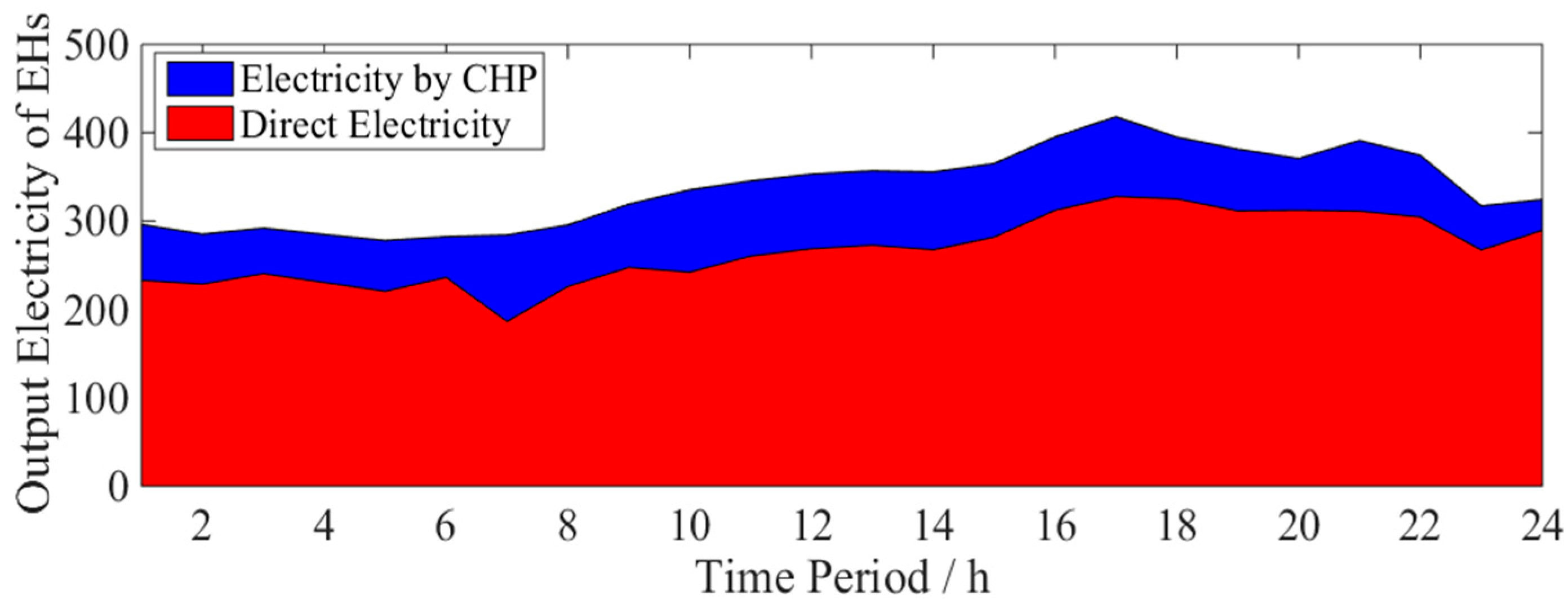
Figure 9 shows the suppliers of output electricity after integrated DR is considered. In this case, the sources of end-users’ electricity demand can be flexible rather than predefined. Energy hubs are able to resort to more economical resources while maintaining users’ satisfaction. Note that during the night (1 h~6 h, 22 h~24 h), less electricity tends to be supplied by CHP since the direct sources from the upper-level system are redundant and with no conversion loss. The portion of electricity demand, supplied by CHP, accounts for 23.6% during the day and decreases to 17.7% during the night.
(3) Case III
Stochastic optimization is simulated in this part to analyze the effect of wind uncertainty on interconnected EHs operation. In this case, the day-ahead scheduling problem is modelled and solved using the proposed scenario-based stochastic formulation. The standard deviation of wind fluctuation is set at 10% of its predicted value. Latin hypercube sampling method is employed to generate 1000 scenarios of hourly wind power, which are further efficiently reduced to 10 selected scenarios within 36.4 s through the backward scenario reduction process.
Solution results are detailly given in Table 2, which present wind power, total operation cost, natural gas cost, wind curtailment, interrupted load, and load shedding of each scenario with corresponding probability. Note that the operation cost of deterministic solution in Case II is $503,440, whereas the expected cost of all the 10 scenarios increases by $180 as wind power uncertainty is considered in Case III. The increment is caused by the overestimation of wind output. In most cases, system energy demands can be fully satisfied without load shedding when the integrated demand response is included. However, the actual wind power over the day is 2289.1 MW and 2307.0 MW in S2 and S9, respectively, which is much lower than the predicted value of 2407.0 MW. In these extreme scenarios, even the introduction of integrated DR cannot guarantee system operation security. This overestimation results that 10.32 MW and 6.74 MW of demand are inevitably shed in S2 and S9 during peak hours, and the operation costs of these two scenarios are hence much higher.
Compared to the computation time in deterministic model (4.08 s in Case I and 6.32 s in Case II), the solution procedure takes much longer as 266.87 s in Case III with 10 retained scenarios. The computation time strongly depends on the scale of optimization model, that is, the number of scenarios. However, few scenarios can deteriorate solution precision. Ten scenarios will be a good tradeoff between the solution efficiency and accuracy.
5.2. Seventeen-Hub Interconnected System
To validate of the proposed model in large-scale systems, numerical test on the seventeen-bub interconnected system is carried in 6 h scheduling window. These EHs are interconnected through a modified RTS-79 power system and two connected Belgian natural gas systems [12]. The test system has 24 electric buses, 40 gas nodes, 12 natural gas-fired units, 17 coal-fired units, and four wind farms. Interruptible DR is not considered in this section. Topology and parameters of the tested system are detailed given in motor.ece.iit.edu/data/ConnectedEH17_stochastic.xlsx.
Based on the five selected scenarios after reduction, results of stochastic programming are given as Table 3. With the consideration of integrated demand response and distributed natural gas storage, the expected operation cost is reduced by 24.8%. Simulation shows that transmission constraint is the main reason for load shedding in our case, more wind power can only benefit in system operation cost, but not load shedding. However, more load will be shed when wind power is not adequate in S3, since thermal units and integrated DR cannot provide sufficient backup in this situation.
Table 4 illustrates the impact of wind penetration level on operation strategy. It is observed that system operation cost can be significantly reduced when wind penetration level is higher (doubled as the base case). The reduction is mainly due to the saving of thermal units’ production. Meanwhile, 253.2 MW wind is curtailed for system security, and the amount of load shedding stays nearly unchanged since the transmission network is in congestion. When wind penetration is reduced by 50%, as in the base case (low level), system operation cost is increased by 11.95% due to the additional generation of thermal units and load shedding increment. Proper penetration of renewable energy like wind power is beneficial to the efficiency of system operation.
Present in Table 5 is the different piecewise strategies, which are compared to test the computation performance of the proposed sequential linearization method. The ideal approximation resolution is set as 1/16 of the range of pipeline gas flow and nodal gas pressure. Without a sequential procedure, the traditional one-time method requires dividing the primal domain into 16 piecewise segments, which introduces so many integer variables that solution efficiency is the worst (>6 h). While these abundant piecewise segments guarantee approximation accuracy, the traditional method is weak in real-time performance, which makes it hard for practical engineering application.
When sequential linearization method is implemented, solution efficiency is greatly improved. Three different piecewise strategies are provided to satisfy the approximation accuracy. In the first case, four rough segments are divided in the first iteration and the total cost is $776,240. In the second iteration, four detailed segments are further divided when the rough operation domain is decided, and system operation costs increases to $776,290—as the ideal traditional method. Due to the far fewer integers in each iteration, the whole solution time is dramatically decreases to 1818.1 s, and the CPU time of the second iteration is a bit shorter since the feasible region has been tightened after precious iteration. In the second case, only two segments are divided in the first iteration and solution results are quick, given as 210.5 s. However, the division strategy is so rough that it may easily lead to local optimal. While another eight segments are divided in the next iteration, the final operation cost is $776,200 and different from the ideal value. In the third case, eight segments are detailly divided in the first iteration and find a precise enough result (total cost is $776,280), but its solution time is much longer than the first strategy (8475.1 s + 144.9 s = 8620.0 s). In our case, the first piecewise strategy is regarded as the best choice, which can avoid local optimal with high solution efficiency. In practical application, operators are suggested to equally divide piecewise segments in each sequential iteration. Moreover, more segments are suggested in the first iteration to avoid local optimal if the time permits.
Table 5 also provides the simulation results through traditional nonlinear model, in which natural gas flow is modelled by concave Weymouth functions and EH input/output relationship is modelled by nonlinear matrix with an unfixed dispatch factor. The nonlinear model is handled by an IPOPT solver. It shows that, due to the strong nonlinearity and nonconvexity of this model, the solution is not converged even after 10 h. The systems total cost is given as $785,360 when the procedure is interrupted at 10 h, which is sub-optimum since the primal model is concave. Global optimal is not guaranteed in this nonlinear model.
6. Conclusions and Future Work
This paper presents a novel stochastic programming framework for the optimal scheduling of interconnected energy hubs, considering integrated demand response and wind power uncertainty. The objective of the proposed model is minimizing the total operation cost, while satisfying end-user’s energy demand. To achieve this objective, integrated DR programs, including internal and external terms, are implemented. The internal DR program is achieved by the optimal operation within each EH, while external DR denotes the adjustment of users’ demand through time-shifting or interruption actions. Distributed natural gas storage is also included to smooth load profile and further improve system efficiency. Moreover, to handle the primal nonlinear nonconvex programming problem, the upper-level transmission network is linearized through the sequential linearization method, while the terminal EH is linearly modelled by an output-input relationship with an augmented coupling matrix. Simulation tests on three-hub and seventeen-hub interconnected system validate the effectiveness of the proposed model and solution methodology.
Based on simulation analysis, following suggestions are provided to system operators and government. Firstly, integrated demand response can benefit a lot in economy improvement reliability enhancement and renewable energy penetration. Detailed and flexible demand response programs are very welcomed in current Energy Internet environment, which can increase the interaction on users’ side and smooth demand curve. Secondly, distributed storage like gas tank can provide a buffer for system operation during peak hours. With the development of storage technology, other forms of storage like large battery, electric vehicle, and the power-to-gas facility can also play important roles in IES operation. Thirdly, wind variation is a main challenge for future energy system with high renewable energy penetration. More accurate wind forecast is needed since load shedding usually occurs when wind power is overestimated. Last but not least, the proposed linearized model and sequential linearization method can provide a feasible solution for IES real-time dispatch. Piecewise segments are suggested to be equally divided in each iteration for both solution efficiency and approximation accuracy reasons.
Our future work will focus on the planning strategy and risk management for interconnected EHs considering the integrated DR program. Other conversion equipment in Energy Internet including electric vehicles, electricity storage, photovoltaics, and the power-to-gas facility will also be comprehensively considered in our further research.
Author Contributions
Y.Z. and C.G. conceived and designed the experiments; Y.Z. and Y.H. performed the experience and analyzed the data. Y.Z. wrote the paper; C.G. conceived the project; Y.H., M.Y., C.G. and Y.D. reviewed and edited the manuscript. All authors read and approved the manuscript.
Funding
The work of Yining Zhang, Yubin He and Chuangxin Guo was supported in part by National Key Research and Development Program of China (2017YFB0902600) and in part by the State Key Program of National Natural Science Foundation of China (51537010).
Conflicts of Interest
The authors declare no conflict of interest.
Nomenclature
A. Sets and Indices
| i, w | Indices of thermal units and wind farms |
| t, s | Indices of time intervals and scenarios |
| h, j | Indices of electricity buses |
| m, n | Indices of natural gas nodes |
| hj, mn | Indices of transmission lines and pipelines |
| sp, q | Indices of natural gas wells and gas storages |
| r | Indices of energy hubs (EH) |
| NP | Sets of piecewise segments of linear cost function for non-NGU |
| NT, GU | Sets of time intervals and natural gas-fired units (NGU) |
| CGj, CEHj | Sets for generators and EHs connected to bus j |
| CUm, CEHm, | Sets for NGUs and EHs connected to node m |
| GWm, GNm, GSm | Sets for gas wells, gas nodes and gas storages connected to node m |
| PLFj PLEj | Sets for transmission lines from/to bus j |
B. Parameters
| Probability of scenario s and price of gas | |
| Penalty of wind curtailment and load shed | |
| Power of wind farm w at time t | |
| Max/min capacity of thermal unit i | |
| Marginal cost of non-NGU i on segment p | |
| Up/down ramping limit of unit i | |
| suci, sdci | Startup/shut cost of non-NGU i |
| sugi, sdgi | Startup/shut gas of NGU i |
| Min ON/OFF time of thermal unit i | |
| xhj | Reactance of transmission line hj |
| Capacity of transmission line hj | |
| Max/min phase angle of bus j | |
| Max/min natural gas production of well sp | |
| Max/min pressure of gas node m | |
| Storing/releasing efficiency of natural gas storage q | |
| Max storing/releasing capacity of natural gas storage q | |
| Max storing/releasing capacity of heat storage in EH r | |
| Max gas and heat stored in storage utility | |
| Max power input of CHP and electric boiler in EH r. | |
| Original energy demand of end-users of EH r at hour t | |
| Max shiftable load of EH r | |
| Max interruptible load of EH r | |
| Cr | Coupling matrix of EH r |
| Efficiency of CHP converting gas to electricity and heat | |
| Efficiency of electric boiler | |
| Storing/releasing efficiency of heat storage | |
| Efficiency of NGU, MW/m3 | |
| Energy conversion constant between gas and electricity, m3/MW | |
| Gas flow/linepack constant of pipeline mn | |
| Capacity and energy compensation for IL |
C. Variables
| Cost of integrated DR program | |
| Linear operation cost function of non-NGU i | |
| Status indicator of thermal unit i at hour t | |
| ON/OFF time counter of unit i at hour t | |
| Generation of thermal unit i at hour t | |
| Startup/shut cost of non-NGU i at hour t | |
| Startup/shut gas of NGU i at hour t | |
| Wind curtailment of wind farm w at hour t | |
| Energy demand shedding of EH r at hour t | |
| Power flow on transmission line hj at hour t | |
| Phase angle of bus j at hour t | |
| Cost/gas consumed by unit i at hour t | |
| Production of natural gas in well sp at hour t | |
| Pressure of gas node m at hour t | |
| Average pressure of pipeline mn at hour t | |
| Average flow, in-flow and out-flow of pipeline mn at hour t | |
| Linepack of pipeline mn at hour t | |
| Total gas load at node m at hour t | |
| Storing/releasing rate of storage q at hour t | |
| Status of storage q at hour t | |
| Natural gas stored in storage q at hour t | |
| Input/output vectors of EH r | |
| Energy of EH r as inputs/outputs at hour t | |
| Energy flows in EH r at hour t | |
| Change of heat storage in EH r at hour t | |
| Status of heat storage in EH r at hour t | |
| Heat stored in EH r at hour t | |
| Energy demand shifted in/out in EH r at hour t | |
| Energy demand interrupted in EH r at hour t |
References
- International Gas Union. IGU World LNG Report—2017 Edition. 2017. Available online: http://www.igu.org/sites/default/files/node-document-field_file/103419-World_IGU_Report_no%20crops.pdf (accessed on 5 April 2017).
- Rifkin, J. The Third Industrial Revolution: How Lateral Power is Transforming Energy, the Economy, and the World; Palgrave Macmillan Trade: New York, NY, USA, 2011; pp. 33–72. ISBN 0230341977. [Google Scholar]
- Geidl, M.; Koeppel, G.; Favre-Perrod, P.; Klockl, B.; Andersson, G.; Frohlich, K. Energy hubs for the future. IEEE Power Energy Mag. 2007, 5, 24–30. [Google Scholar] [CrossRef]
- Shahidehpour, M.; Fu, Y.; Wiedman, T. Impact of natural gas infrastructure on electric power systems. Proc. IEEE 2005, 93, 1042–1056. [Google Scholar] [CrossRef]
- Li, T.; Eremia, M.; Shahidehpour, M. Interdependency of natural gas network and power system security. IEEE Trans. Power Syst. 2008, 23, 1817–1824. [Google Scholar] [CrossRef]
- Wang, C.; Wei, W.; Wang, J.H.; Liu, F.; Qiu, F.; Correa-Posada, C.M.; Mei, S.W. Robust defense strategy for gas-electric systems against malicious attacks. IEEE Trans. Power Syst. 2017, 32, 2953–2965. [Google Scholar] [CrossRef]
- Shao, C.C.; Shahidehpour, M.; Wang, X.F.; Wang, X.L.; Wang, B.Y. Integrated planning of electricity and natural gas transportation systems for enhancing the power grid resilience. IEEE Trans. Power Syst. 2017, 32, 4418–4429. [Google Scholar] [CrossRef]
- Bai, L.Q.; Li, F.X.; Jiang, T.; Jia, H.J. Robust scheduling for wind integrated energy systems considering gas pipeline and power transmission N-1 contingencies. IEEE Trans. Power Syst. 2017, 32, 1582–1584. [Google Scholar] [CrossRef]
- Correa-Posada, C.M.; Sánchez-Martın, P. Security-constrained optimal power and natural-gas flow. IEEE Trans. Power Syst. 2014, 29, 1780–1787. [Google Scholar] [CrossRef]
- Wen, Y.F.; Qu, X.B.; Li, W.Y.; Liu, X.; Ye, X. Synergistic operation of electricity and natural gas networks via ADMM. IEEE Trans. Smart Grid 2018, 9, 4555–4565. [Google Scholar] [CrossRef]
- He, Y.B.; Yan, M.Y.; Shahidehpour, M.; Li, Z.Y.; Guo, C.X.; Wu, L.; Ding, Y. Decentralized optimization of multi-area electricity-natural gas flows based on cone reformulation. IEEE Trans. Power Syst. 2018, 33, 4531–4542. [Google Scholar] [CrossRef]
- Borraz-Sanchez, C.; Bent, R.; Backhaus, S.; Hijazi, H.; Hentenryck, P. Convex relaxations for gas expansion planning. Inf. J. Comput. 2016, 28, 645–656. [Google Scholar] [CrossRef]
- Correa-Posada, C.M.; Sánchez-Martın, P. Integrated power and natural gas model for energy adequacy in short-term operation. IEEE Trans. Power Syst. 2015, 30, 3347–3355. [Google Scholar] [CrossRef]
- Urbina, M.; Li, Z.Y. A combined model for analyzing the interdependency of electrical and gas systems. In Proceedings of the 39th North American Power Symposium (NAPS), Las Cruces, NM, USA, 30 September–2 October 2007. [Google Scholar]
- Feng, Q.; Wen, F.S.; Liu, X.Y.; Salam, M.A. A residential energy hub model with a concentrating solar power plant and electric vehicles. Energies 2017, 10, 1159. [Google Scholar] [CrossRef]
- Huang, Y.N.; Guo, C.X.; Ding, Y.; Wang, L.C.; Zhu, B.Q.; Xu, L.Z. A multi-period framework for coordinated dispatch of plug-in electric vehicles. Energies 2016, 9, 370. [Google Scholar] [CrossRef]
- Zheng, Y.; Hill, D.J.; Dong, Z.Y. Multi-agent optimal allocation of energy storage systems in distribution systems. IEEE Trans. Sustain. Energy 2017, 8, 1715–1725. [Google Scholar] [CrossRef]
- Shabanpour-Haghighi, A.; Seifi, A.R. Energy flow optimization in multi-carrier systems. IEEE Trans. Ind. Inform. 2015, 11, 1067–1077. [Google Scholar] [CrossRef]
- Dolatabadi, A.; Mohammadi-Ivatloo, B.; Abapour, M.; Tohidi, S. Optimal stochastic design of wind integrated energy hub. IEEE Trans. Ind. Inform. 2017, 13, 2379–2388. [Google Scholar] [CrossRef]
- Zhou, X.Z.; Guo, C.X.; Wang, Y.F.; Li, W.Q. Optimal expansion co-planning of reconfigurable electricity and natural gas distribution systems incorporating energy hubs. Energies 2017, 10, 124. [Google Scholar] [CrossRef]
- Zhang, X.P.; Shahidehpour, M.; Alabdulwahab, A.; Abusorrah, A. Optimal expansion planning of energy hub with multiple energy infrastructures. IEEE Trans. Smart Grid 2015, 6, 2302–2311. [Google Scholar] [CrossRef]
- Wang, Y.; Zhang, N.; Kang, C.Q.; Kirschen, D.S.; Yang, J.W.; Xia, Q. Standardized matrix modeling of multiple energy systems. IEEE Trans. Smart Grid 2017. [Google Scholar] [CrossRef]
- Wang, Y.; Zhang, N.; Zhuo, Z.Y.; Kang, C.Q.; Kirschen, D.S. Mixed-integer linear programming-based optimal configuration planning for energy hub: Starting from scratch. Appl. Energy 2018, 210, 1141–1150. [Google Scholar] [CrossRef]
- Geidl, M.; Andersson, G. Optimal power flow of multiple energy carriers. IEEE Trans. Power Syst. 2007, 22, 145–155. [Google Scholar] [CrossRef]
- Moeini-Aghtaie, M.; Abbaspour, A.; Fotuhi-Firuzabad, M.; Hajipour, E. A Decomposed solution to multiple-energy carriers optimal power flow. IEEE Trans. Power Syst. 2014, 29, 707–716. [Google Scholar] [CrossRef]
- Moeini-Aghtaie, M.; Dehghanian, P.; Fotuhi-Firuzabad, M.; Abbaspour, A. Multiagent genetic algorithm: An online probabilistic view on economic dispatch of energy hubs constrained by wind availability. IEEE Trans. Sustain. Energy 2014, 5, 699–708. [Google Scholar] [CrossRef]
- Yang, S.C.; Zeng, D.; Ding, H.F.; Yao, J.G.; Wang, K.; Li, Y.P. Stochastic security-constrained economic dispatch for random responsive price-elastic load and wind power. IET Gener. Transm. Distrib. 2016, 10, 936–943. [Google Scholar] [CrossRef]
- Wu, H.Y.; Shahidehpour, M.; Alabdulwahab, A. Hourly demand response in day-ahead scheduling for managing the variability of renewable energy. IET Gener. Transm. Distrib. 2013, 7, 226–234. [Google Scholar] [CrossRef]
- Zhang, X.P.; Shahidehpour, M.; Alabdulwahab, A.; Abusorrah, A. Hourly electricity demand response in the stochastic day-ahead scheduling of coordinated electricity and natural gas networks. IEEE Trans. Power Syst. 2016, 31, 592–601. [Google Scholar] [CrossRef]
- Liu, N.; He, L.; Yu, X.H.; Ma, L. Multiparty energy management for grid-connected microgrids with heat- and electricity-coupled demand response. IEEE Trans. Ind. Inform. 2018, 14, 1887–1897. [Google Scholar] [CrossRef]
- Shao, C.Z.; Ding, Y.; Wang, J.H.; Song, Y.H. Modelling and integration of flexible demand in heat and electricity integrated energy system. IEEE Trans. Sustain. Energy 2018, 9, 361–370. [Google Scholar] [CrossRef]
- Hu, J.H.; Wen, F.S.; Wang, K.; Huang, Y.C.; Salam, M.A. Simultaneous provision of flexible ramping product and demand relief by interruptible loads considering economic incentives. Energies 2018, 11, 46. [Google Scholar] [CrossRef]
- Wang, J.X.; Zhong, H.W.; Ma, Z.M.; Xia, Q.; Kang, C.Q. Review and prospect of integrated demand response in the multi-energy system. Appl. Energy 2017, 202, 772–782. [Google Scholar] [CrossRef]
- Odetayo, B.; Kazemi, M.; Maccormack, J.; Rosehart, W.D.; Zareipour, H.; Seifi, A.R. A chance constrained programming approach to the integrated planning of electric power generation, natural gas network and storage. IEEE Trans. Power Syst. 2018. [Google Scholar] [CrossRef]
- He, Y.B.; Shahidehpour, M.; Li, Z.Y.; Guo, C.X.; Zhu, B.Q. Robust constrained operation of integrated electricity-natural gas system considering distributed natural gas storage. IEEE Trans. Sustain. Energy 2018, 9, 1061–1071. [Google Scholar] [CrossRef]
- Wu, L.; Shahidehpour, M.; Li, Z.Y. Comparison of scenario-based and interval optimization approaches to stochastic SCUC. IEEE Trans. Power Syst. 2012, 27, 913–921. [Google Scholar] [CrossRef]
- Rastegar, M.; Fotuhi-Firuzabad, M.; Zareipour, H.; Moeini-Aghtaieh, M. A probabilistic energy management scheme for renewable-based residential energy hubs. IEEE Trans. Smart Grid 2017, 8, 2217–2227. [Google Scholar] [CrossRef]
- Li, Y.; Zou, Y.; Tan, Y.; Cao, Y.J.; Liu, X.D.; Shahidehpour, M.; Tian, S.M.; Bu, F.P. Optimal stochastic operation of integrated low-carbon electric power, natural gas, and heat delivery system. IEEE Trans. Sustain. Energy 2018, 9, 273–283. [Google Scholar] [CrossRef]
- Ma, X.Y.; Sun, Y.Z.; Fang, H.L. Scenario generation of wind power based on statistical uncertainty and variability. IEEE Trans. Sustain. Energy 2013, 4, 894–904. [Google Scholar] [CrossRef]
- Elia. Wind-Power Generation Data. 2018. Available online: http://www.elia.be/en/grid-data/power-generation/wind-power (accessed on 4 June 2018).
Figure 1.
Typical topology of the interconnected Energy hubs.

Figure 2.
The schematic of integrated demand response.

Figure 3.
Flowchart of solving the proposed stochastic model for interconnected EHs.

Figure 4.
Topology of three-hub interconnected system.
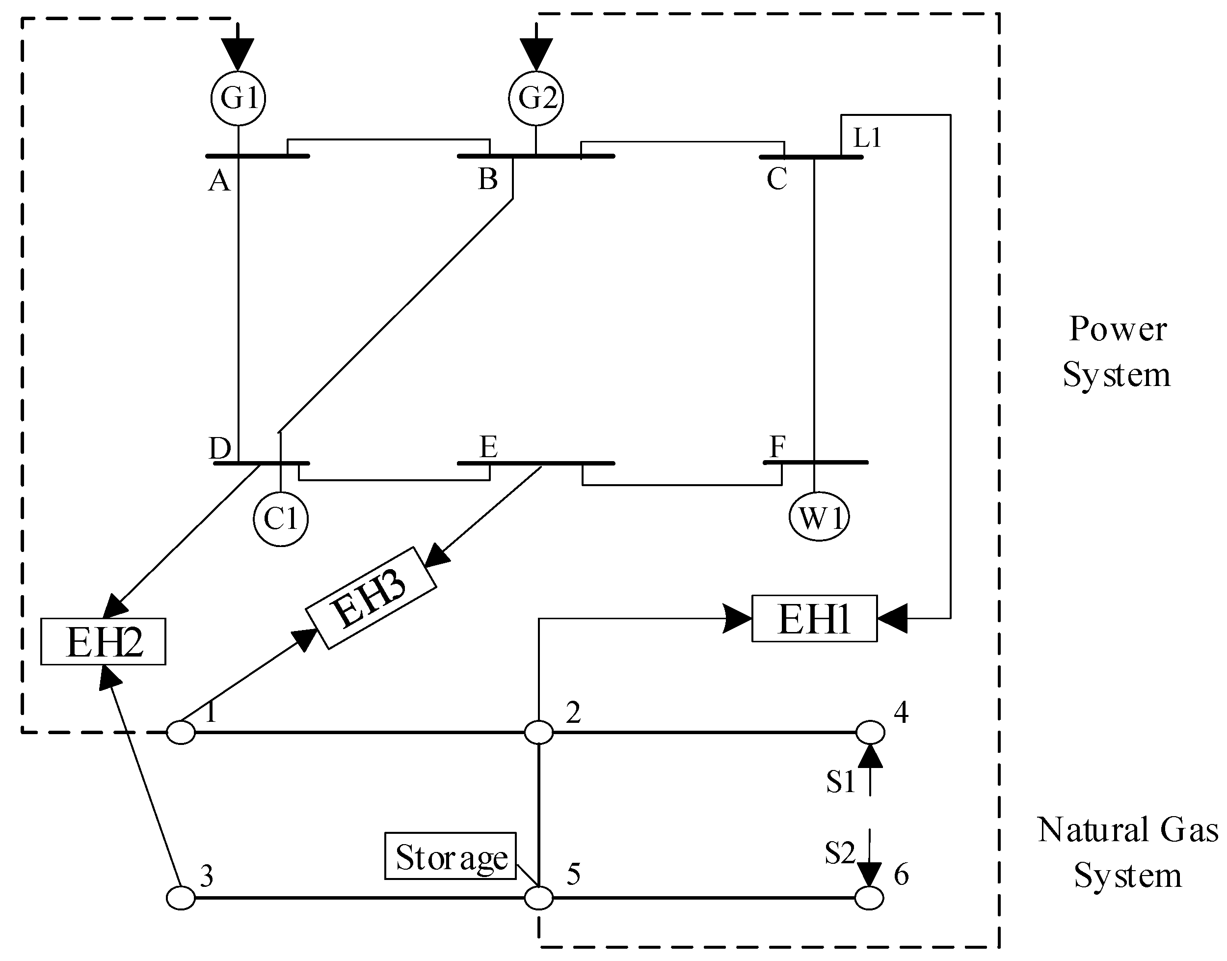
Figure 5.
Energy resources in transmission level.
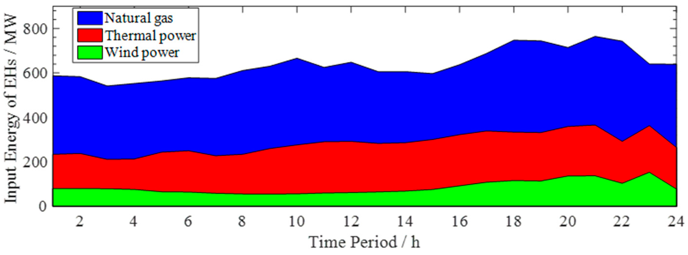
Figure 6.
Suppliers of heat demand in EHs.

Figure 7.
Profile of stored natural gas and total system load.

Figure 8.
Load profile with and without integrated demand response.
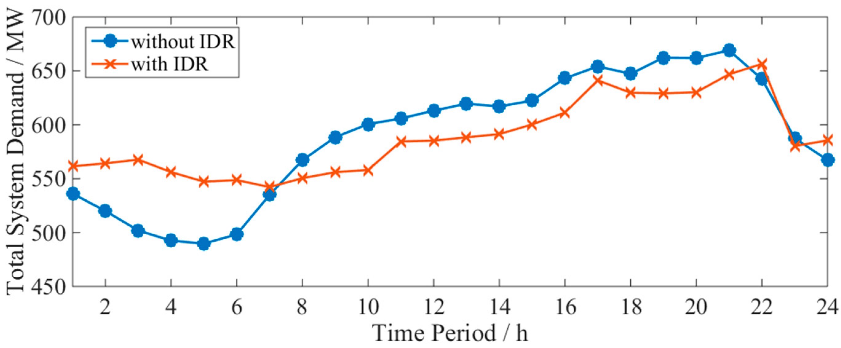
Figure 9.
Suppliers of electricity demand in energy hubs.


Table 1.
Comparison between different demand response (DR) strategies.
| DR strategy | Total Cost ($) | Coal Cost ($) | Natural Gas Cost ($) | Curtailed Wind (MW) | Interrupted Load (MW) | Shed Load (MW) |
|---|---|---|---|---|---|---|
| Case I | 918,980 | 49,338 | 432,000 | 725.81 | 0 | 423.12 |
| (Without DR) | ||||||
| Case II.a | 816,240 | 49,338 | 422,020 | 435.26 | 0 | 336.12 |
| (Internal DR only) | ||||||
| Case II.b | 670,530 | 49,338 | 422,470 | 223.66 | 457.94 | 148.40 |
| (External DR only) | ||||||
| Case II.c | 503,440 | 49,338 | 423,870 | 116.58 | 278.51 | 0 |
| (Integrated DR) |
Table 2.
Results of different wind uncertainty scenarios.
| Expected Cost of the Ten Scenarios: $503,620 | |||||||
|---|---|---|---|---|---|---|---|
| Scenario | Probability | Wind Power (MW) | Total Cost ($) | Gas Cost ($) | Curtailed Wind (MW) | Interrupted Load (MW) | Shed Load (MW) |
| S1 | 0.169 | 2387.4 | 501,760 | 423,030 | 75.92 | 278.15 | 0 |
| S2 | 0.030 | 2289.1 | 515,440 | 424,930 | 62.76 | 295.46 | 10.32 |
| S3 | 0.189 | 2482.1 | 501,430 | 421,920 | 143.18 | 272.52 | 0 |
| S4 | 0.074 | 2425.6 | 503,320 | 423,780 | 132.46 | 275.02 | 0 |
| S5 | 0.062 | 2406.9 | 504,640 | 425,050 | 145.75 | 272.84 | 0 |
| S6 | 0.159 | 2367.4 | 505,470 | 425,360 | 114.33 | 284.35 | 0 |
| S7 | 0.053 | 2410.0 | 503,370 | 423,910 | 120.34 | 276.67 | 0 |
| S8 | 0.149 | 2454.8 | 502,170 | 423,260 | 148.82 | 265.42 | 0 |
| S9 | 0.032 | 2307.0 | 511,040 | 424,210 | 57.53 | 295.46 | 6.74 |
| S10 | 0.083 | 2397.8 | 503,970 | 424,060 | 111.93 | 282.76 | 0 |
Table 3.
Results of different wind uncertainty scenarios.
| Expected Cost of the Five Scenarios: $776,290 | |||||||
|---|---|---|---|---|---|---|---|
| Scenario | Probability | Wind Power (MW) | Total Cost ($) | Coal Cost ($) | Gas Cost ($) | Shed Load (MW) | Curtailed Wind (MW) |
| S1 | 0.252 | 1670.5 | 775,130 | 196,190 | 569,720 | 9.22 | 0 |
| S2 | 0.338 | 1658.1 | 776,070 | 197,130 | 569,720 | 9.22 | 0 |
| S3 | 0.104 | 1603.0 | 779,440 | 198,080 | 569,720 | 11.64 | 0 |
| S4 | 0.140 | 1652.5 | 776,030 | 197,090 | 569,720 | 9.22 | 0 |
| S5 | 0.166 | 1628.0 | 776,750 | 197,810 | 569,720 | 9.22 | 0 |
Table 4.
Results under different wind penetration levels.
| Wind Penetration | Total Cost ($) | Wind Curtailment (MW) | Shed Load (MW) |
|---|---|---|---|
| Low Level | 869,060 | 0 | 55.32 |
| Base Level | 776,290 | 0 | 9.44 |
| High Level | 683,630 | 253.2 | 9.41 |
Table 5.
Efficiency of the proposed sequential linearization method.
| Results of the Traditional Method (16) | ||||
| Iteration | Total Cost ($) | Flow Segments (Integers) | Pressure Segments (Integers) | CPU Time (s) |
| 1 | 776,290 | 16 * NGL * NT | 16 * NGB * NT | 23574.7 |
| Results of the proposed method in strategy 1 (4 * 4 = 16) | ||||
| Iteration | Total Cost ($) | Flow Segments (Integers) | Pressure Segments (Integers) | CPU Time (s) |
| 1 | 776,240 | 4 * NGL * NT | 4 * NGB * NT | 941.9 |
| 2 | 776,290 | 4 * NGL * NT | 4 * NGB * NT | 876.2 |
| Results of the proposed Method in strategy 2 (2 * 8 = 16) | ||||
| Iteration | Total Cost ($) | Flow Segments (Integers) | Pressure Segments (Integers) | CPU Time (s) |
| 1 | 776,170 | 2 * NGL * NT | 2 * NGB * NT | 210.5 |
| 2 | 776,200 | 8 * NGL * NT | 8 * NGB * NT | 6510.4 |
| Results of The Proposed Method in Strategy 3 (8 * 2 = 16) | ||||
| Iteration | Total cost ($) | Flow segments (Integers) | Pressure segments (Integers) | CPU time (s) |
| 1 | 776,280 | 8 * NGL * NT | 8 * NGB * NT | 8475.1 |
| 2 | 776,290 | 2 * NGL * NT | 2 * NGB * NT | 144.9 |
| Results of the Traditional Nonlinear Model | ||||
| Iteration | Total Cost ($) | Flow Segments (Integers) | Pressure Segments (Integers) | CPU Time (s) |
| 1 | 785,360 (sub-optimum) | - | - | >10 h (not converged) |
Noted that it still takes about half an hour for solution, the solution speed can be further improved by techniques like identifying inactive constraints and generating strong Benders cuts.
© 2018 by the authors. Licensee MDPI, Basel, Switzerland. This article is an open access article distributed under the terms and conditions of the Creative Commons Attribution (CC BY) license (http://creativecommons.org/licenses/by/4.0/).
Share and Cite
MDPI and ACS Style
Zhang, Y.; He, Y.; Yan, M.; Guo, C.; Ding, Y. Linearized Stochastic Scheduling of Interconnected Energy Hubs Considering Integrated Demand Response and Wind Uncertainty. Energies 2018, 11, 2448. https://doi.org/10.3390/en11092448
AMA Style
Zhang Y, He Y, Yan M, Guo C, Ding Y. Linearized Stochastic Scheduling of Interconnected Energy Hubs Considering Integrated Demand Response and Wind Uncertainty. Energies. 2018; 11(9):2448. https://doi.org/10.3390/en11092448
Chicago/Turabian StyleZhang, Yining, Yubin He, Mingyu Yan, Chuangxin Guo, and Yi Ding. 2018. "Linearized Stochastic Scheduling of Interconnected Energy Hubs Considering Integrated Demand Response and Wind Uncertainty" Energies 11, no. 9: 2448. https://doi.org/10.3390/en11092448
Note that from the first issue of 2016, this journal uses article numbers instead of page numbers. See further details here.