Deploying Electric Vehicle Charging Stations Considering Time Cost and Existing Infrastructure


1
State Key Laboratory of Automotive Safety and Energy, Department of Automotive Engineering, Tsinghua University, Beijing 100084, China
2
Collaborative Innovation Center of Electric Vehicles in Beijing, Beijing 100081, China
*
Author to whom correspondence should be addressed.
Energies 2018, 11(9), 2436; https://doi.org/10.3390/en11092436
Submission received: 30 August 2018
/
Revised: 7 September 2018
/
Accepted: 10 September 2018
/
Published: 14 September 2018
(This article belongs to the Section A: Sustainable Energy)
Abstract
:Under the challenge of climate change, fuel-based vehicles have been receiving increasingly harsh criticism. To promote the use of battery electric vehicles (BEVs) as an alternative, many researchers have studied the deployment of BEVs. This paper proposes a new method to choose locations for new BEV charging stations considering drivers’ perceived time cost and the existing infrastructure. We construct probability equations to estimate drivers’ demanding time for charging (and waiting to charge), use the Voronoi diagram to separate the study area (i.e., Shanghai) into service areas, and apply an optimization algorithm to deploy the charging stations in the right locations. The results show that (1) the probability of charging at public charging stations is 39.6%, indicating BEV drivers prefer to charge at home; (2) Shanghai’s central area and two airports have the busiest charging stations, but drivers’ time costs are relatively low; and (3) our optimization algorithm successfully located two new charging stations surrounding the central area, matching with our expectations. This study provides a time-efficient way to decide where to build new charging stations to improve the existing infrastructure.
1. Introduction
As greenhouse gasses increasingly affect the environment and human life, countries around the globe have been trying to reduce gas emissions. One approach is to replace fuel-based vehicles with battery electric vehicles (BEVs). However, the deployment of BEVs is a challenging issue [1]. It requires strategic planning to locate the right number of charging stations (and piles) in the right locations [2]. Since studies give different weights to different constraints (e.g., BEV energy consumption, electric grid stability, land availability, and investment costs), the deployment results are different. However, there are two common targets: one is to estimate the demand for charging stations and the other is to minimize the costs to meet that demand. The demand for charging stations may be due to population growth, increase of GDP per capita, or infrastructure lifecycle [3,4,5]. To meet an increasing demand usually requires additional costs, e.g., investment costs, operation costs, and maintenance costs. Researchers usually employ objective functions [6] to minimize these costs by minimizing missed trips [7], BEV energy consumption [8,9], travel distance, and so on.
Since the deployment of charging stations is largely subject to geographic constraints, a number of studies included graph theories to their analysis [10]. For example, in the study of minimizing energy consumption of BEVs to reach the next charging station, a group of researchers adopted a weighted Voronoi diagram to calculate the size and shape of the service areas [8,9]. Similarly, another group of researchers used graph theories to minimize the investment costs, operation costs, and users’ costs [10,11]. They have defined users’ costs as waiting plus travelling time to the next charging station. It is understandable that studies involving geographic dimensions (e.g., distance) adopt graph theories to enhance the efficiency of their solutions.
To locate the right number of charging stations (and piles) in the right locations, a number of researchers adopted the particle swarm optimisation algorithm to minimize costs. For example, Liu et al. [7] applied particle swarm optimisation to solve a non-convex, non-linear combinatorial objective function while considering the investment costs of charging piles. The authors considered the number of BEVs, types of users, types of charging, battery characteristics, charging time, and charging environment as influencing factors. Similarly, Xu et al. [8] applied a binary particle swarm optimisation algorithm to determine the optimal configuration for central charging stations by minimizing the total travel distance to these central stations.
From the literature review, we can see that previous studies have not taken into account drivers’ time cost for waiting to charge, which is an excellent indicator for demand. In other words, if drivers have to wait a long time to charge, the corresponding service area needs additional charging stations (or piles). Moreover, when locating the charging stations, previous studies mostly did not take into account the layout of existing public charging stations. The existing charging stations in a city form a network system. Intuitively, we claim that considering the existing layout when adding new nodes to a system can minimize the disturbance to the system.
Therefore, this paper aims to consider the layout of existing charging stations to determine the locations for new BEV charging stations that minimize drivers’ time cost. Using Shanghai City as an example, we estimate the demanding times for charging and waiting to charge at each existing charging station. After identifying the service areas with the highest time cost, we add new stations to those areas to reduce the costs. Additionally, the flourishing degree of corresponding areas represented by the commercial prosperity index is taken into consideration to determine the optimal location where these newly-built charging stations are placed. We also demonstrate the investment costs involved in constructing new charging stations (and piles).
2. Model Specification
2.1. Drivers’ Charging Behaviour
It takes time to charge a BEV. Drivers first park their vehicles and then charge. We use Equations (1) and (2) to estimate the time for a BEV to be fully charged:
where is the required time for a full recharge, is the th parking event, SOC is the state of charge, and is the average C-rate charging for the battery based on SOC. Specifically:
where is the charging current, and is the battery capacity.
Secondly, we separate a charging event from a parking event. When drivers have parked their vehicles, they may not charge or not fully charge their vehicles. For the former, we use a discrete probability distribution to represent drivers’ probability to charge their vehicles (i.e., ). For the latter, we compare the parking time with the required time for a full recharge (i.e., ). Therefore, we obtain the demanding time for charging (i.e., ) through Equations (3) and (4):
where is the time for charging at the th parking event, is the demanding time for charging at the th parking event, and is the probability of charging at public infrastructure with a specific SOC.
Thirdly, we consider drivers’ lingering and waiting times at a parking event. Lingering happens when drivers park their vehicles longer than the required time for a full recharge (i.e., ). We obtain the demanding time for waiting to charge through Equations (5) and (6):
where is the time for waiting to charge at the th parking event, and is the demanding time for waiting to charge the th parking event.
Finally, we use a vector to represent the demanding times for charging and for waiting to charge during each of the 24 h in a day, as shown in Equation (7). If an event spans multiple days, we split the event into different vectors for each day:
where is the demanding time vector for charging, and is the demanding time vector for waiting to charge.
2.2. Locating Charging Stations
We use the Voronoi diagram to locate new charging stations because it guarantees reasonable separation of the existing charging stations into service areas. As we learned from literature, there is no perfect separation method in graph theory. Note that a charging station may have multiple charging piles; therefore, the capacities of charging stations are not the same.
The Voronoi diagram is named after the Russian mathematician G. Voronoi. Preparate and Shamos [12] explained the diagram as follows: Given a set S of N points on a plane, the diagram divides the plane into N polygons. For every point pj, the locus of points is closer to pj than to any other point. For two points , the set of points closer to pj than to pk is a half-plane defined by the perpendicular bisector of pj pk. This half-plane is denoted as H (pj, pk). The locus of points closer to pj than to any other point, denoted as Vor(j), is the intersection of N-1 half-planes. Vor(j) is the Voronoi polygon associated with pj, as shown in Equation (8). Vor(S) is the Voronoi diagram for the N points, as shown in Figure 1:
In this study, we consider an existing or new station as a point and the point’s Voronoi polygon as the station’s service area. We use Equations (9)–(11) to estimate the demanding time for charging in each service area. In Equation (11), the numerator represents the sum of demanding time in service area j, and the denominator represents the number of charging piles in service area j. Therefore, represents the demanding time for charging in service area j. For example, if , we can say that for an hour on average, a charging pile in this service area has 21 min (0.35 × 60) in use (for charging). Apparently, the will be smaller with more charging piles in a service area.
where is the aggregated demanding time for charging in service area j on day t; is the demanding time vector for charging in service area j on day t; is the averaged demanding time for charging during time period ; is the average hourly distribution of demanding time for charging in each service area; and is the number of charging piles at service area .
Similarly, we can calculate the demanding time for waiting to charge in each service area, as shown in Equations (12)–(14). Therefore, we can estimate the demanding time for each service area in any given period. The hourly distribution vectors help to understand drivers’ charging behaviours in any location at any time:
where is the aggregated demanding time for waiting to charge in service area j on day t, is the demanding time vector for waiting to charge in service area j on day t, is the averaged demanding time for waiting to charge during time period , and is the average hourly distribution of demanding time for waiting to charge in each service area.
2.3. Optimisation Algorithm
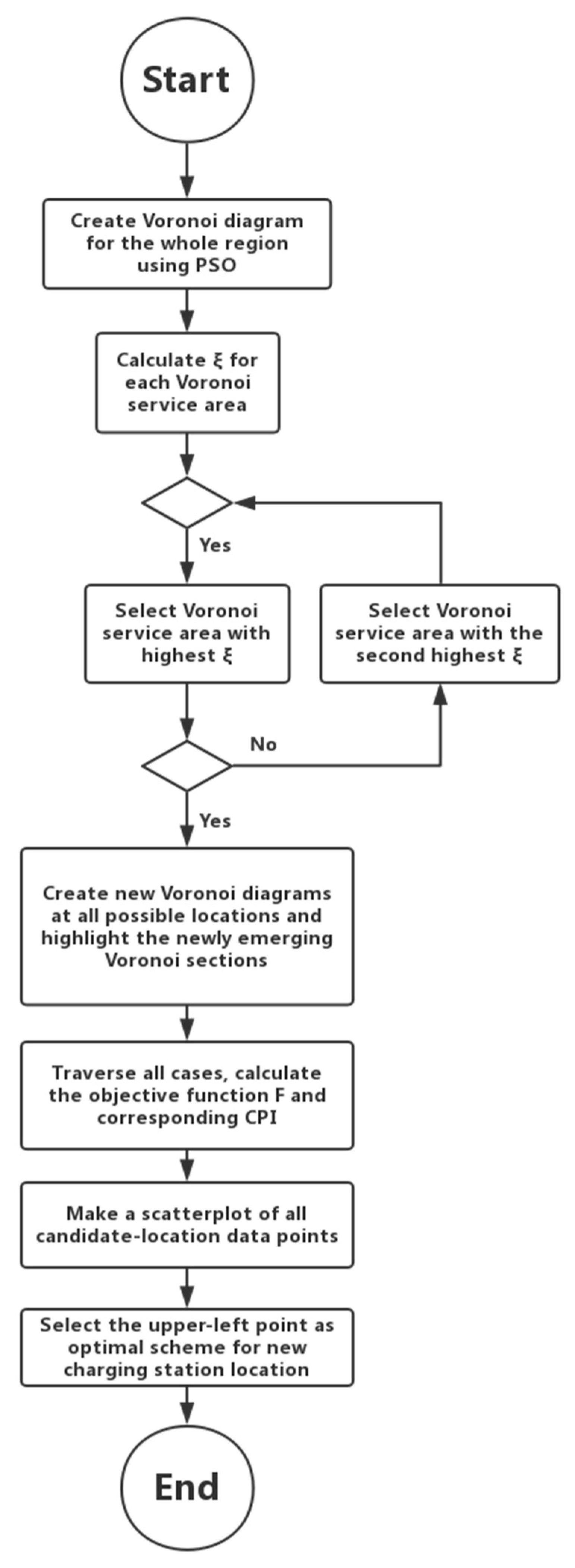
In this section, we demonstrate an optimisation algorithm to minimize drivers’ time cost. In Section 2.1 and Section 2.2, we have simulated drivers’ charging behaviour in service areas through their time of using (or waiting to use) the charging piles. To reduce the time cost, we need to add additional charging piles. This section demonstrates an algorithm to reach an optimal solution.
Figure 2 shows a unified modelling language (UML) activity diagram for the algorithm. First, the algorithm creates a Voronoi diagram for all existing charging stations. Applying Equation (14), the algorithm calculates an averaged demanding time for waiting to charge (i.e., ) for each service area. We define the service area with the largest value of (i.e., as having the highest potential to locate a new station. However, the service area corresponding to may not be qualified for a new station due to municipality regulations. For example, Shanghai only allows its new charging stations to be built within existing parking lots. In other words, if a service area has no parking lot, it cannot have any new charging station no matter how large the value of is. In this case, the algorithm will move to the next largest . Note that when we add a new charging station, the number of service areas becomes , and the algorithm updates the values of and .
Mathematically, we can denote the set of service areas with existing parking lots as E. Equation (15) checks whether there are candidate locations within the service areas with large :
where L is the set of candidate locations for new charging stations, E is the set of service areas with existing parking lots, and is the th service area.
If the service area the largest has parking lots, we will traverse all the parking lots in this service area. The parking lot that satisfies our objective function will be chosen as the optimal location for a new charging station. The objective is to minimize the time cost as described in Equation (16). Note that the overall expenditure is not set as a constraint parameter in the algorithm to give infrastructure planners more flexibility. We also surveyed the BEV drivers to estimate the weights for the demanding time for charging (i.e., ) and the demanding time for waiting to charge (i.e., ). The sum of the two weights is equal to one. Then we averaged the weights, which gives a value of 0.3 and a value of 0.7. Apparently, BEV drivers care more about the demanding time for waiting to charge (i.e., 0.7) than for charging (i.e., 0.3). We think BEV drivers’ opinions should be considered in the time cost analysis, so we introduce the two weights in the objective function, as follows:
where is the drivers’ perceived time cost at charging stations, is the number of charging stations, is the weight of demanding time for charging, and is the weight of demanding time for waiting to charge. Considering that BEV drivers generally have the expectation of making good use of the spare time during the process of waiting to get charged and getting charged, the surroundings of candidate locations are supposed to be employed as a quantitative criterion for deploying newly-built charging stations. With the same drivers’ perceived time cost , candidate location adjacent to more shopping malls, cinemas, and office buildings will be given higher priority for the sake of BEV drivers’ convenience. Based on the profound analysis data of different hierarchical commercial areas in Shanghai [13,14,15], the commercial prosperity index (CPI) is brought in as an indicator of the flourishing degree of every candidate location. Various influence factors such as visitors’ flowrate, rent, space, and living standard of the surrounding residents are integrated into account to obtain the commercial prosperity index. In consequence it can be regarded as an objective and synthetic evaluation index [16,17].
As shown in Figure 3, each black dot represents one candidate location in the Voronoi service area. The horizontal axis represents the average drivers’ perceived time cost per hour . The vertical axis represents the commercial prosperity index (CPI). Obviously, the closer the black dot is to the top left corner of the graph, the smaller the time cost and the higher CPI, which means he corresponding candidate location can provide BEV drivers with comparatively less waiting time and more work or entertainment choices. Therefore, the black dot in the red circle will be selected as the optimal scheme. Moreover, the overall expenditure is calculated using the following equation:
where
is the overall expenditure, is the investment cost per simple charging station, is the investment cost per standardized slow charging pile, is the desired number of new charging stations to build and is the number of charging piles per station.
Finally, we use the particle swarm algorithm [18] and display the results through a web tool. The algorithm is well known because it uses simple concepts, few parameters, and fast convergence. It has been widely used in engineering practice and function optimisation, especially for grid partition and regional segmentation [19,20,21].
3. The Case of Shanghai
3.1. Data
In this study, data sources include AutoNavi Software Co., Ltd (a Chinese web mapping company acquired by Alibaba Group), Potevio Group Corporation (a Chinese high-tech research company), EV Power Holding Limited (a Hong Kong-based company specializing in charging solutions), and Bavarian Motor Works (BMW, a German luxury car maker). AutoNavi provides the data of existing public charging stations as well as GPS tracking data. We use the most recent GPS tracking data for Shanghai, which contains 378 vehicles and 28,247 parking events from 1–31 January 2017. Potevio provides the number of Potevio charging stations, and EV Power provides the number of EV Power charging stations, as well as the charging stations’ parking (charging) data recorded at each charging pile. There are 86 Potevio charging stations and 32 EV Power charging stations in Shanghai, as shown in Figure 4. BMW (control cloud) provides rather complete monitoring data (e.g., vehicle current status, vehicle speed, SOC, charging voltage, and current). Table 1 is a simplified version, for example.
3.2. The Result of Charging Behaviour
In this section, we apply the proposed model in Shanghai, China. Figure 5 shows the probability density function. The total probability for public charging is 39.6%, whereas the total probability for private charging is 60.4%. This result matches with that of Morrissey et al. [11]. Specifically, for a SOC below 20%, drivers are more likely to charge their vehicles at public charging stations. This is probably because they could not reach home with the remaining battery. For a SOC above 20%, drivers are more likely to charge at private charging stations. The probability gradually decreases, starting from a SOC of 30% for both charging scenarios.
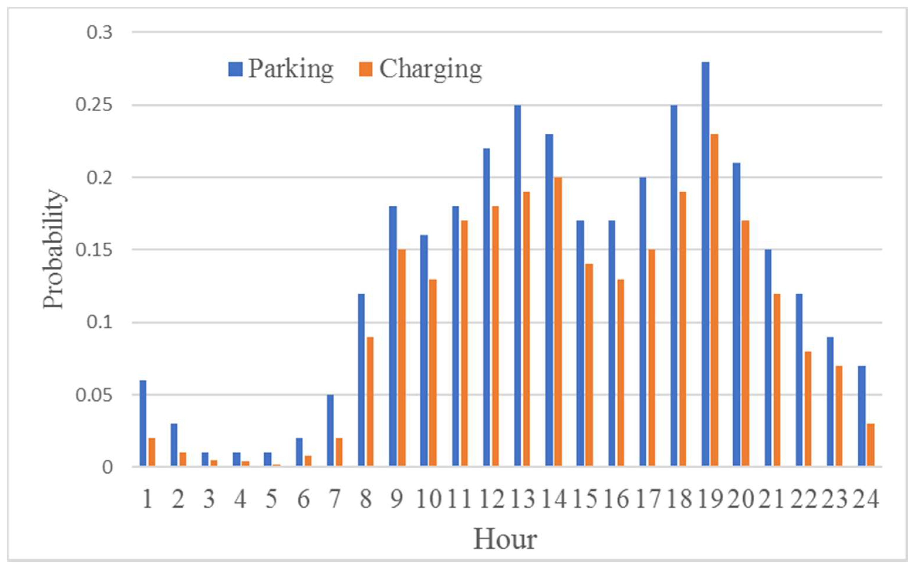
Figure 6 displays an example of drivers’ charging behaviour at a random charging pile. The horizontal axis represents 24 h of one day, and the 1st hour is 0:00–1:00 a.m. The vertical axis represents the probability of an event (parking or charging) occurring in this hour. For example, we can see from this figure that in the 18th hour, the parking probability is 0.25, while the charging probability is 0.19. That is, from 17:00–18:00 p.m., all the parking events recorded by this single charging pile amount to 15 min (, and all the charging events amount to 11.4 min. Apparently, this example charging pile is not busy, as it is not fully occupied by BEVs during each period of time in the whole day.
Figure 7 shows the parking event heat-map for Shanghai in January 2017. The red colour indicates the busiest (i.e., most occupied) parking lots, followed by the yellow, green, and blue colours sequentially. In general, the city’s central area has busy parking lots, as well as two airports (shown with an airplane symbol).
3.3. The Result of Identifying Potential Locations
Figure 8 shows the service areas for the existing charging stations in Shanghai. Each dot in green, yellow, blue, and red shows the position of the charging stations. Their colours represent the hourly-averaged waiting time (i.e., value) for a pile in a charging station. Note that there is only one charging station in one Voronoi polygon.
Although the parking lots in the central area are busy, the hourly-averaged waiting time per pile () in the service areas is not long, probably because there are enough charging piles. In the outskirts, the values of are larger, probably because there are not enough charging piles in these areas.
3.4. The Result of the Optimisation Algorithm
The quality of infrastructure usually increases with the investment cost. To compromise between time cost and investment cost, we developed the optimisation algorithm in Section 2.3. In this section, we used Shanghai as an example to demonstrate the application and evaluate the results. According to Potevio and EV Power [22,23,24,25], in Shanghai is set to 350,000 renminbi (RMB), and , is set to 25,000 RMB, as shown in Table 2.
In most parking lots in Shanghai City, if the parking time is less than 15 min, one need not pay for the parking fee. Therefore, we set the as 15 min. That is, if an observed event in the monitor data (provided by the BMW control cloud) is less than 15 min, then we do not consider it as a parking event and the relative data will not be taken into calculation.
Figure 9 shows the optimized service areas. We can see the placement of the potential charging stations. The green dots with a white cross in the centre mark the position of the new charging stations, and the areas with deep green boundaries define their service areas. Compared with the initial situation shown in Figure 8, the original blue area and a nearby yellow area were substituted by green service areas that have lower time costs. Additionally, the original red area shrunk.
One might wonder why these two new stations were not placed within the red area in Southwest Shanghai. This may be due to the lack of parking lots in the area. Since the new charging stations can only be placed within existing parking lots in Shanghai, the algorithm selected the next best option, which is close to the red area.
However, we have only collected the driving data from 378 BMW BEVs in Shanghai and BEV charging data provided by Potevio and EV Power. These data sources have not covered all BEVs in Shanghai. Understandably, our results have under-estimated the demand for charging stations (and piles) in Shanghai.
4. Discussion and Conclusions
This study estimates the demand for charging stations and charging piles considering drivers’ time cost and existing infrastructure. We first simulate the drivers’ possibility of charging at public infrastructure and the probability to charge rather than park the BEVs. Next, we calculate the demanding time for charging and waiting to charge during each hour in a day (for a total of 24 h). Then, we use the Voronoi diagram to create a service area for each of the existing charging stations in Shanghai. After identifying the service area with the highest time cost, our algorithm adds additional charging stations to reduce the time cost. Finally, we estimate the investment cost for these new charging stations and piles.
The result shows that drivers’ probability for charging at public stations is 39.6%, whereas the probability for charging at home is 60.4%. This result matches with the results of Morrissey et al. [11]. Taking into account the SOC, we conclude that drivers prefer to charge at home and only charge at public infrastructure when the remaining battery is not enough for them to reach home.
Our algorithm correctly chooses the areas that lack charging stations. Although the parking event heat-map shows that the busy parking lots in Shanghai are located in the central area, the optimisation algorithm chose the areas surrounding the central area for locating new charging stations. This is reasonable because the time cost for charging (and waiting) is low in the central areas since there are many charging stations. In the surrounding area, there are much fewer charging stations and the urban expansion is ongoing. We are confident that the algorithm has chosen the correct locations for locating new charging stations.
The application of a time-of-use electricity pricing system makes the charging price an influence factor of the BEV drivers’ choices. However, the charging price has been the same throughout the day in Shanghai until now. Additionally, supported by relevant policy, the charging price in Shanghai is set relatively low to promote the development of BEVs. According to our survey of BEV drivers, the charging price is not a key point compared with the waiting time and the surroundings of the charging station. Therefore, the influence of variable price is not taken into consideration when constructing the model. With the development of BEVs in Shanghai and other Chinese cities, a peak-valley electricity price system may be widely applied in many places, thus, corresponding revisions will have to be made for further research.
Finally, the proposed models in this study provide a comprehensive scheme for infrastructure planners to estimate the demand for charging stations based on available data provided by electronic vehicle research companies. With the fast development of these high-tech companies, we expect to integrate data for all vehicles in a region in the near future. Using the models proposed in this paper, we could allocate new charging stations in a most time-efficient way and, at the same time, improve the existing infrastructure network.
Author Contributions
Conceptualization: K.H. and Y.Q.; Methodology: J.Q. and K.H.; Software: J.Q. and Y.S.; Formal analysis: Y.Q. and J.J.; Data curation: Y.Q. and J.Q.; Writing—original draft preparation: Y.Q.; Writing—review and editing: K.H. and Y.Q.
Funding
This research was funded by Beijing Municipal Science and Technology Commission, grant number D17111000490000, and the BMW China Heat Map Analytics GeoDB Project.
Acknowledgments
The authors gratefully acknowledge the administrative and technical support from the AutoNavi Software Co., Ltd, Potevio Group Corporation, EV Power Holding Limited, and BMW China.
Conflicts of Interest
The authors declare no conflict of interest.
References
- Haddadian, G.; Khodayar, M.; Shahidehpour, M. Accelerating the global adoption of electric vehicles: Barriers and drivers. Electr. J. 2015, 28, 53–68. [Google Scholar] [CrossRef]
- Trigg, T.; Telleen, P.; Boyd, R.; Cuenot, F.; D’Ambrosio, D.; Gaghen, R.; Gagné, J.; Hardcastle, A.; Houssin, D.; Jones, A. Global EV outlook: Understanding the electric vehicle landscape to 2020. Int. Energy Agency 2013, 1, 1–40. [Google Scholar]
- Dong, J.; Liu, C.; Lin, Z. Charging infrastructure planning for promoting battery electric vehicles: An activity-based approach using multiday travel data. Transp. Res. Part C Emerg. Technol. 2014, 38, 44–55. [Google Scholar] [CrossRef]
- Ge, S.; Feng, L.; Liu, H. The planning of electric vehicle charging station based on Grid partition method. In Proceedings of the 2011 International Conference on Electrical and Control Engineering, Yichang, China, 16–18 September 2011; pp. 2726–2730. [Google Scholar]
- Tang, Z.; Guo, C.; Hou, P.; Fan, Y. Optimal siting of electric vehicle charging stations based on voronoi diagram and FAHP method. Energy Power Eng. 2013, 5, 1404–1409. [Google Scholar] [CrossRef]
- Jia, L.; Hu, Z.; Liang, W.; Lang, W.; Song, Y. A novel approach for urban electric vehicle charging facility planning considering combination of slow and fast charging. In Proceedings of the 2014 International Conference on Power System Technology, Chengdu, China, 20–22 October 2014; pp. 3354–3360. [Google Scholar]
- Liu, Z.; Zhang, W.; Ji, X.; Li, K. Optimal planning of charging station for electric vehicle based on particle swarm optimization. In Proceedings of the IEEE PES Innovative Smart Grid Technologies, Tianjing, China, 16–20 January 2012; pp. 1–5. [Google Scholar]
- Xu, H.; Miao, S.; Zhang, C.; Shi, D. Optimal placement of charging infrastructures for large-scale integration of pure electric vehicles into grid. Int. J. Electr. Power. 2013, 53, 159–165. [Google Scholar] [CrossRef]
- Zhao, L.; Xie, M.; Dong, J.; Zheng, Z.; Wang, X. Electric vehicle charging facility planning in Shenzhen Power Supply Bureau Limited Company. In Proceedings of the 2012 IEEE International Electric Vehicle Conference, Greenville, SC, USA, 4–8 March 2012; pp. 1–5. [Google Scholar]
- Zheng, Y.; Dong, Z.Y.; Xu, Y.; Meng, K.; Zhao, J.H.; Qiu, J. Electric vehicle battery charging/swap stations in distribution systems: Comparison study and optimal planning. IEEE Trans. Power Syst. 2014, 29, 221–229. [Google Scholar] [CrossRef]
- Morrissey, P.; Weldon, P.; O’Mahony, M. Future standard and fast charging infrastructure planning: An analysis of electric vehicle charging behaviour. Energy Policy 2016, 89, 257–270. [Google Scholar] [CrossRef]
- Preparata, F.P.; Shamos, M.I. Computational Geometry: An Introduction; Springer Science & Business Media: New York, NY, USA, 2012. [Google Scholar]
- Wang, D.; Wang, C.; Xie, D.; Zhong, W.; Min, W.U.; Zhu, W.; Zhou, J.; Yuan, L.I. Comparison of Retail Trade Areas of Retail Centers with Different Hierarchical Levels: A Case Study of East Nanjing Road, Wujiaochang, Anshan Road in Shanghai. Urban Plan. Forum 2015, 3, 50–60. [Google Scholar] [CrossRef]
- Zhong, W.; Wang, D.; Xie, D.; Yan, L. Dynamic characteristics of Shanghai's population distribution using cell phone signaling data. Geogr. Res. 2017, 36, 972–984. [Google Scholar] [CrossRef]
- Mingxiao, L.I.; Chen, J.; Zhang, H.; Qiu, P.; Liu, K.; Feng, L.U. Fine-grained Population Estimation and Distribution Characteristics in Shanghai. J. Geo-Inf. Sci. 2017, 19, 800–807. [Google Scholar] [CrossRef]
- Huang, P. The comprehensive measure of agglomeration characteristics of commercial sites in central city of Shanghai. J. Hubei Univ. 2016, 38, 572–578. [Google Scholar] [CrossRef]
- Ma, L.; Wang, D.; Zhu, W. In Research on Residents’ Shopping behavior in Mega-community of Shanghai Suburban New Town. In Proceedings of the National Planning Conference, Seattle, WA, USA, 18–21 April 2015. [Google Scholar]
- Tversky, A.; Kahneman, D. Rational choice and the framing of decisions. J. Bus. 1986, 59, S251–S278. [Google Scholar] [CrossRef]
- Kahneman, D. Maps of bounded rationality: Psychology for behavioral economics. Am. Econ. Rev. 2003, 93, 1449–1475. [Google Scholar] [CrossRef]
- Dantzig, G.B.; Thapa, M.N. Linear Programming 2: Theory and Extensions; Springer Science & Business Media: New York, NY, USA, 2006. [Google Scholar]
- De Berg, M.; Van Kreveld, M.; Overmars, M.; Schwarzkopf, O. Computational geometry. In Computational Geometry; Springer: Berlin, Germany, 1997; pp. 1–17. [Google Scholar]
- Shanghai Municipal Electric Power Company; Shanghai Jiao Tong University; Shanghai Electric Power Design Institute Co. Construction Specifications for Electric Vehicles' Charging Infrastructure in Shanghai; DG/TJ08-2093-2012; Shanghai Construction and Transportation Committee: Shanghai, China, 2012. [Google Scholar]
- AC Charging Product Specifications. Available online: http://www.evpowergroup.com/page5.php?n=3/ (accessed on 16 May 2017).
- Charging Infrastructure Products Introduction. Available online: http://www.ptne.cn/contents/39/1278.html (accessed on 18 May 2017).
- Zheng, J.; Mehndiratta, S.; Guo, J.Y.; Liu, Z. Strategic policies and demonstration program of electric vehicle in China. Transp. Policy (Oxf.) 2012, 19, 17–25. [Google Scholar] [CrossRef] [Green Version]
Figure 1.
(a) Voronoi polygon, Vor(j); and (b) Voronoi diagram, Vor(S).
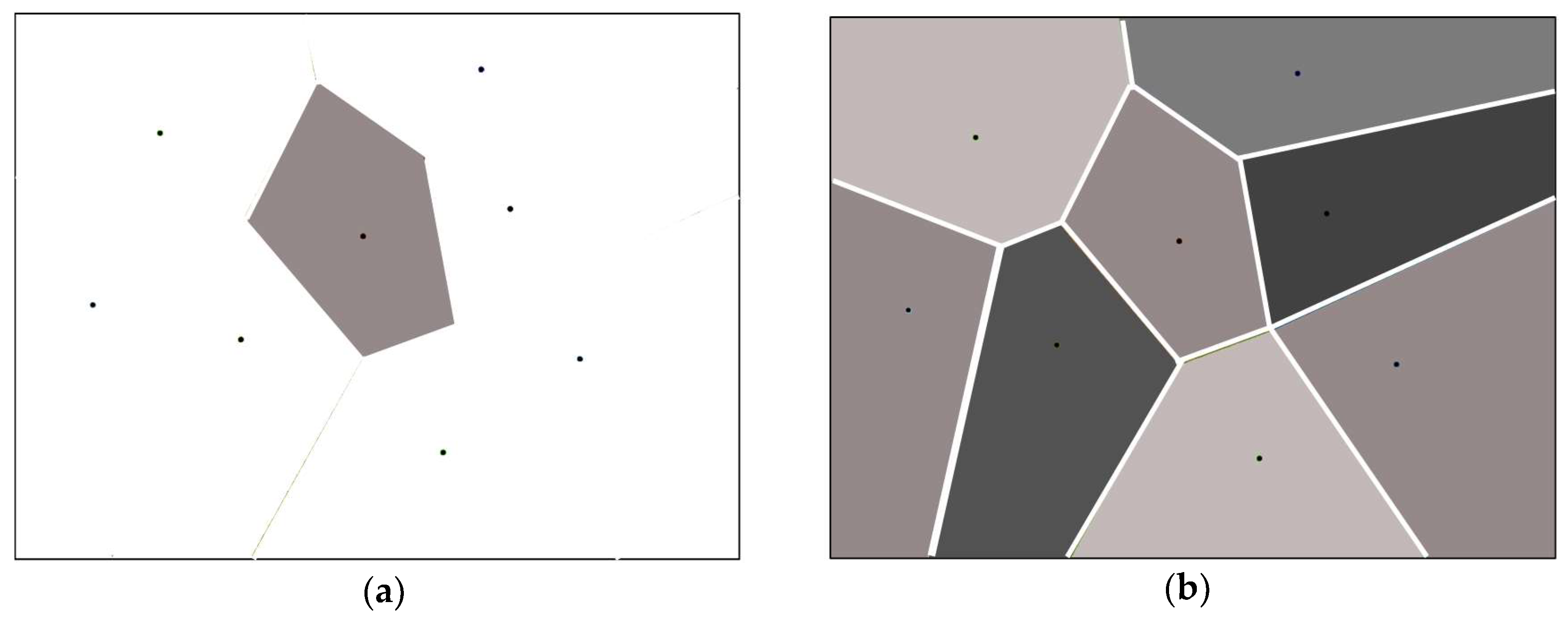
Figure 2.
UML activity diagram for the optimisation algorithm. PSO: particle swarm optimisation.

Figure 3.
Calculation results of candidate locations in the Voronoi service area.
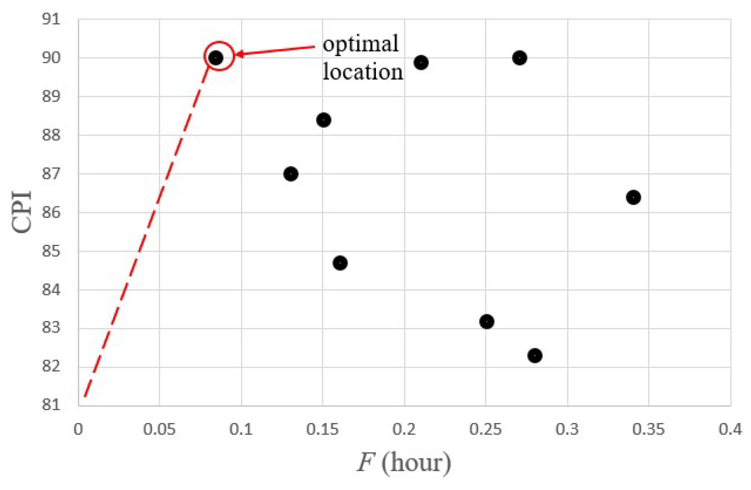
Figure 4.
Locations of existing charging stations in Shanghai.
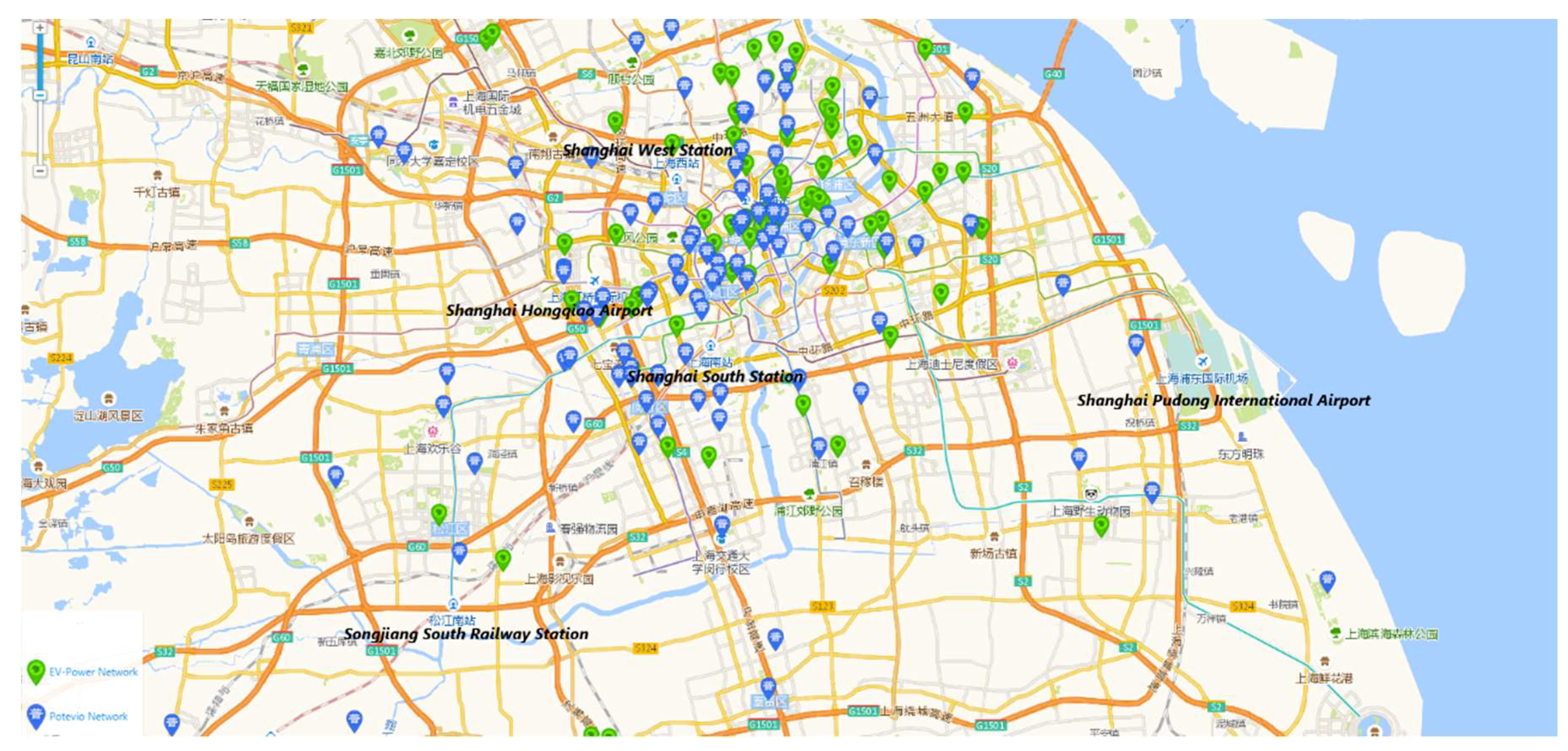
Figure 5.
Probability density functions for private and public charging.

Figure 6.
Distribution of parking and charging events at a single charging pile.

Figure 7.
Parking event heat-map.
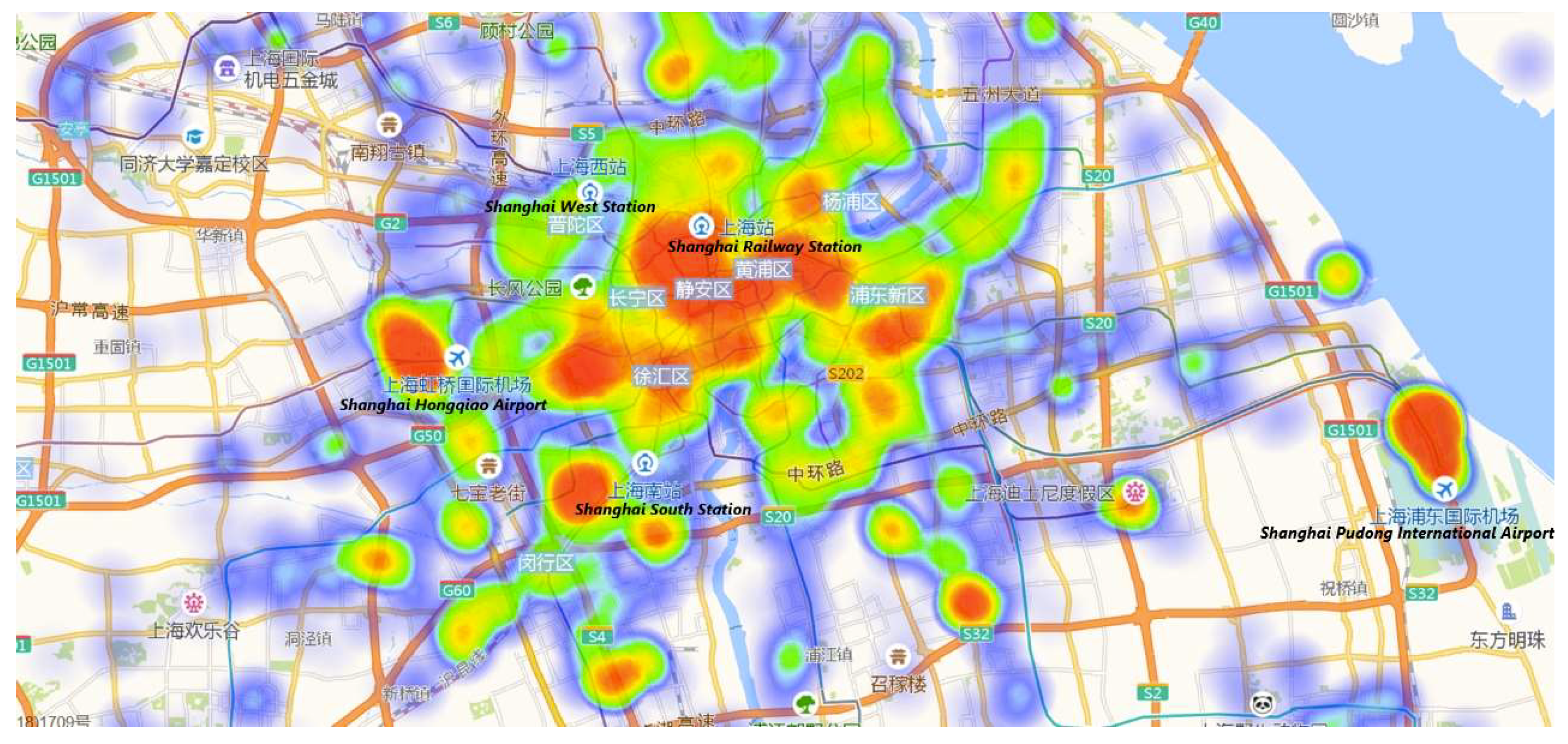
Figure 8.
Service areas for existing stations.

Figure 9.
Identifying potential locations for charging stations.


Table 1.
Simplified version of BEV driving data provided by BMW.
| BEV-ID | Date | Time | SOC (%) | Vehicle Speed (km/h) | Vehicle Current Status | Charging/Discharging Status | Charging Voltage (V) | Charging Current (A) |
|---|---|---|---|---|---|---|---|---|
| 5 | 30 January 2017 | 16:20:16 | 24 | 3.2 | Running | Discharging | 0 | 0 |
| 5 | 30 January 2017 | 16:22:21 | 22 | 1.6 | Running | Discharging | 0 | 0 |
| 5 | 30 January 2017 | 16:23:21 | 19 | 0.4 | Stopped | Discharging | 0 | 0 |
| 5 | 30 January 2017 | 16:29:52 | 27 | 0.0 | Charging | Charging | 216 | 2.8 |
Table 2.
Input parameters for the optimisation.
| Parameter | Unit | Value |
|---|---|---|
| RMB | 350,000 | |
| RMB | 25,000 | |
| / | 2 | |
| / | 4 | |
| Minutes | 15 | |
| / | 0.3 | |
| / | 0.7 |
© 2018 by the authors. Licensee MDPI, Basel, Switzerland. This article is an open access article distributed under the terms and conditions of the Creative Commons Attribution (CC BY) license (http://creativecommons.org/licenses/by/4.0/).
Share and Cite
MDPI and ACS Style
Qiao, Y.; Huang, K.; Jeub, J.; Qian, J.; Song, Y. Deploying Electric Vehicle Charging Stations Considering Time Cost and Existing Infrastructure. Energies 2018, 11, 2436. https://doi.org/10.3390/en11092436
AMA Style
Qiao Y, Huang K, Jeub J, Qian J, Song Y. Deploying Electric Vehicle Charging Stations Considering Time Cost and Existing Infrastructure. Energies. 2018; 11(9):2436. https://doi.org/10.3390/en11092436
Chicago/Turabian StyleQiao, Yuan, Kaisheng Huang, Johannes Jeub, Jianan Qian, and Yizhou Song. 2018. "Deploying Electric Vehicle Charging Stations Considering Time Cost and Existing Infrastructure" Energies 11, no. 9: 2436. https://doi.org/10.3390/en11092436
Note that from the first issue of 2016, this journal uses article numbers instead of page numbers. See further details here.