Transmission Expansion Planning under Uncertainty for Investment Options with Various Lead-Times

1
Department of Electric and Computer Engineering, Seoul National University, 1 Gwanak-ro, Gwanak-gu, Seoul 06974, Korea
2
Department of Energy System Engineering, Chung-Ang University, 84 Heukseok-ro, Dongjak-gu, Seoul 06974, Korea
*
Author to whom correspondence should be addressed.
Energies 2018, 11(9), 2429; https://doi.org/10.3390/en11092429
Submission received: 23 July 2018
/
Revised: 11 September 2018
/
Accepted: 12 September 2018
/
Published: 13 September 2018
(This article belongs to the Special Issue Electric Power Systems Research 2018)
Abstract
:Investment options of transmission expansion planning (TEP) involve different lead times according to their length, technology, and environmental and social impacts. TEP planners can utilize the various lead times to deal with the risk of uncertainty. This paper proposes a novel framework for TEP under an uncertain environment, which includes investment options with various lead times. A multi-stage model is developed to reflect the different lead times in the planning method. The level of demand uncertainty is represented using a relative standard deviation. Demand uncertainty in the presented multi-stage model and its influence on the optimal decision are studied. The problem is formulated as a mixed integer linear problem to which stochastic programming is applied, and the proposed framework is illustrated from case studies on a modified Garver’s six-bus system. The case studies verify the effectiveness of the framework for TEP problems with a mathematically tractable model and demonstrates that the proposed method achieves better performance than other methods when the problems involve investment candidates with various lead times under uncertain conditions.
1. Introduction
Recently, the increasing integration of new components, such as variable energy resources, energy storage systems, and electric vehicles, has indicated a new direction for temporally managing system resources. Modern power systems are incorporating temporal characteristics of the components in their operation and planning strategies. Accordingly, many research areas regarding temporal characteristics have been actively studied. Primary frequency reserves provided by wind turbines and energy storage systems were studied in Reference [1], and an optimal control strategy to increase the utilization of wind power curtailment was proposed. The impact of wind energy integration on power systems was investigated in Reference [2]. The power reserve requirements required for wind energy integration were estimated at the regional level. In Reference [3], the strategic operation of wind power plants was presented to provide energy and flexible ramping products. The optimization problem decides the operation scheduling of wind power generation in a real-time market. A unit commitment (UC) problem including uncertainty of wind power and solar power was studied in Reference [4]. The presented methodology for solving the UC problem was tested on a 24-h UC test system. Similar studies in transmission expansion planning (TEP) have gained less attention, although various transmission investment options have considered different time schedules in their planning. The impact of different lead times on TEP problems is studied in this research.
Transmission planning activities are divided into several steps according to reliability criteria, while evaluating long-term reliability of transmission networks requires statistical approaches. The amount of load shedding is one of the reliability criteria. An objective function minimizes the sum of the investment cost and expected load-shedding cost [5]. Another reliability criterion is loss of load expectation [6], in which two probabilistic reliability criteria were applied to transmission planning activity: the transmission system and its bus/nodal framework. Deterministic reliability criteria are usually used to evaluate the operating reliability of a transmission network, and the (N-α) contingency criterion is the most widely used method to evaluate the security of transmission networks [7]. To circumvent investigating the whole contingency set, an adjustable robust optimization approach was proposed in Reference [8]. Recent changes in power generation mix require that operating reliability criteria incorporate the characteristics of renewable energy sources. Uncertainty regarding wind power generation was considered in transmission network expansion planning [9], where a combined Monte Carlo and probabilistic power flow analysis method was used with a chance-constrained approach. The interactions of wind power generation and dynamic thermal ratings of transmission lines were investigated in Reference [10], and the authors suggested that constructing new transmission corridors may not be the optimal transmission network reinforcement strategy when wind power generation is connected. Fault analysis and stability analysis are usually the final steps of transmission planning activities [11]. The technical analysis requires a pre-optimized network configuration and different types of parameters for generation and transmission. In this step, the engineering feasibility of the pre-optimized configuration of a transmission network is investigated. This paper focuses on the long-term characteristics of transmission networks under uncertain environments. The expected cost of load shedding is utilized as a reliability criterion.
Planning problems are generally divided into two broad categories: static and dynamic. Static planning has a single decision stage, planning lead time, and a target year. In contrast, dynamic planning has multiple decision stages and target years. This is also called multi-period or multi-stage planning in TEP research. Dynamic planning problems reflect real-world planning processes, where planning decisions are conducted in multiple stages, but have been generally solved by decomposing them into a sequence of static problems or by using heuristic methods owing to computational complexity issues [12]. A heuristic method was used to reduce the combinatorial search space of a multi-stage problem [13]. The strategy is to solve the multi-stage problem by utilizing the solutions of several static problems. A genetic algorithm was used to solve a multi-stage planning problem in Reference [14]. Although the optimal solution of the heuristic method was suboptimal, the results produced lower investment costs than static planning. The aforementioned studies concentrated on the method for reducing the computational complexity inherent in multi-stage problems and did not consider different lead times of investment options. This paper presents a new multi-stage model in which the lead times are reflected to solve transmission planning problems with diverse investment options. The model is a mixture of static and dynamic planning models, capturing the advantages of multiple decision stages in the dynamic model, and mathematical tractability in the static model.
Transmission network investment has many aspects: capital-intensive, long payback period, economy of scale, investment irreversibility, long-run uncertainty, and low adaptability. Especially, long-run uncertainty leads to greater risk for planners and investors [15]. Investing in generating units involves the same problem as investing in transmission networks; however, the former uses market and financial instruments to hedge some of the risk, while there is a lack of such instruments for the latter [16]. Thus, transmission network planners have the crucial role of appropriately dealing with uncertainties in the planning process. Accordingly, long-term uncertainty has been actively studied in the framework of TEP processes to enable planners to cope with risk [17]. The long-term uncertainty in TEP is caused by various sources: demand, generation expansion, market rules, availability of facilities, etc. Among these, demand uncertainty has been considered as one of the most decisive factors in TEP problems. In Reference [18], the authors used robust optimization to find the worst case in a given interval of possible demand values. In Reference [19], long-term demand uncertainty was modeled by a generalized version of a deterministic peak demand.
To incorporate the various characteristics of uncertainty, stochastic approaches have also been used in planning problems. Long-term uncertainty in demand was represented as a Markov chain to take into account the autocorrelation of demand variation on a planning horizon [20]. The demand uncertainty was modeled to follow a discrete probability distribution, and it was applied to a stochastic dynamic programming for generation investment. In Reference [21], the authors addressed the forecasting uncertainty of peak loads in generation and transmission planning. The uncertainty was considered using a normal probability distribution with constant values for demand growth and standard deviation. In Reference [22], scenario construction was applied to take into account long-term demand uncertainty. A chance-constrained programming approach has been introduced to model various uncertain factors in static TEP [23]. The authors modeled demand growth and its uncertainty using normal probability distributions. In Reference [24], a stochastic dynamic model was used in a real option approach to take long-term uncertainty in load growth into account for generation investment optimization. These stochastic approaches captured diverse characteristics of the long-term demand uncertainty, such as autocorrelation, independency, and the mixture of uncertain sources. However, all the stochastic models above were either used in a static TEP or multi-stage TEP involving a regular interval.
TEP practices also involve the process of evaluating the impact of long-term uncertainty. Under restructured electric market environments, generation expansion planning has become a decentralized planning process where private investors seek to gain profit in electricity markets while TEP remains a centralized process [25]. However, the new environment has changed some aspects of TEP activities. In some power systems, private investors are allowed to propose a plan for transmission reinforcement and expansion for limited applications, although the complete process remains within the overall framework of centralized planning [26]. As the complexity of power systems increases, coordination of planning activities becomes more important. The European network of transmission system operators (ENTSO-e), which aims at achieving a coordinated pan-European approach to electricity system planning, releases their ten-year network development plan (TYNDP) every two years [27]. The TYNDP includes a scenario building process to deal with the risks of long-term uncertainty. PJM, a regional transmission organization in the United States, also follows a scenario planning process in its regional transmission planning [28]. The procedure examines the impact of long-term uncertainty on the reliability of the PJM system.
Considering various transmission investment options and their lead times, there have been various methods proposed to deal with the risk of the long-term uncertainty. An optimal decision of flexible alternating current transmission systems (FACTS) investment in the framework of a TEP problem was studied using a real option approach [29]. In Reference [30], the authors considered diverse candidates, such as phase-shifting transformers, energy storage, and others as transmission investment options. The periods needed to build the various investment options were included in the study. In Reference [22], the authors incorporated the duration of transmission construction into the adaptation cost function of a proposed flexible TEP framework. In Reference [31], coordination of construction periods of transmission lines, FACTS, and generators was investigated. Various investment candidates considered in this research may include high voltage AC transmission line construction as well as other methods for expanding transmission capacity, such as FACTS, high voltage DC, and AC to DC conversion. Technical aspects of these various planning options are not considered. Instead, the proposed TEP framework considers the diverse investment candidates in terms of their transmission capacities and lead times.
This paper proposes a novel framework for TEP problems with transmission investment options involving diverse lead times. The various lead times provide the planner with decision choices at different time steps for the network configuration of a target year. A multi-stage model is presented to reflect the advantage of incorporating different lead times in the optimal plan. Long-term uncertainty of peak demand is modeled using the relative standard deviation. The uncertainty model reflects demand variations on the planning horizon, enabling the consideration of uncertainty variation in the decision stages. The demand uncertainty in the proposed multi-stage model and its influence on the optimal decision were studied in the transmission expansion planning problem. The proposed framework is formulated as a mixed integer nonlinear problem. To solve these problems, the nonlinear constraints are replaced by a linear constraint and stochastic programming is applied to the problem. Monte Carlo simulations and sample average approximation are utilized to obtain the deterministic equivalent of the stochastic problem. The main contribution of this paper is presenting a planning framework that reflects different lead times for investment options using a mathematically tractable optimization process.
2. Proposed Framework
2.1. Multi-Stage Model
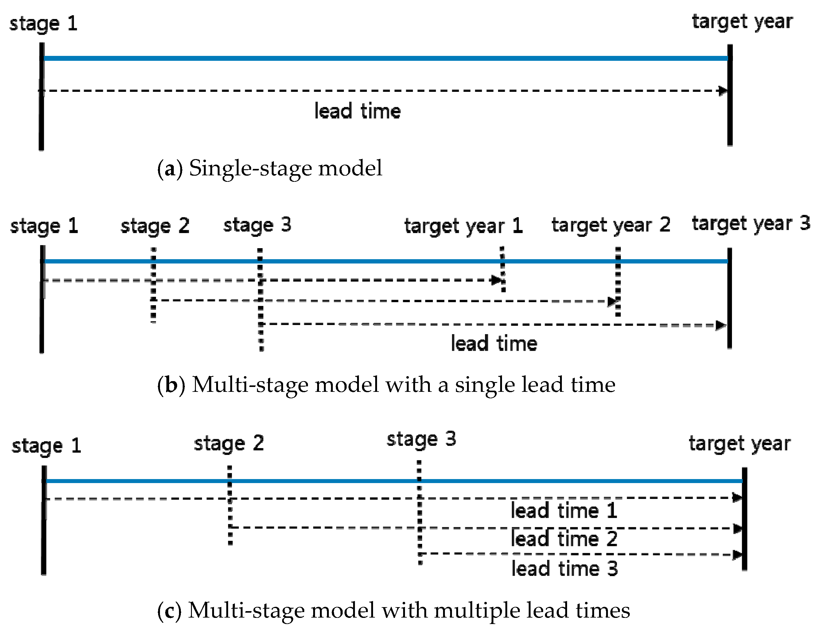
In TEP problems, a stage model plays a crucial role because it may reflect time steps of decisions, target years, and lead times. Various stage models are shown in Figure 1. The model in Figure 1a shows a traditional single stage model used in static planning problems. It has a single decision stage, lead time, and target year. On the other hand, Figure 1b represents an example of a multi-stage model. The model reflects the TEP process, which is conducted on a regular interval assuming that every investment candidate of the transmission planning process has the same lead time for its construction. However, in the real world, investment candidates may have different lead times owing to several reasons, such as the period of construction, the process of gaining right-of-way, the assessment of environmental impact, and the settlement of social issues. The model shown in Figure 1c considers them by setting multiple stages according to the different lead times. In the model, investment decisions take place at multiple stages for the network configuration of a target year.
The models of both Figure 1b,c have multiple decision stages. However, the model in Figure 1c is different from the model in Figure 1b in that each investment candidate is considered only at a single stage. In other words, investment candidates with different lead times belong to different decision stages. This model allows the proposed problem to require less computational complexity than dynamic TEP problems with the stage model in Figure 1b, because the complexity of the dynamic decisions is not reflected in the multi-stage model shown in Figure 1c. Therefore, in our work, the model in Figure 1c was used to reflect the different lead times for the proposed framework.
Investment decisions are made at each time step of the multiple stages, so forecasting of peak demand for the target year also takes place at each time step. Transmission network planners need to utilize all the necessary information available at the initial stage where the planning process begins. Although the exact peak demand of the target year forecasted at time steps of the middle stages is not foreknown, the level of forecasting uncertainty may be known at the initial stage because the extent of the uncertainty can be estimated from historical data as a function of forecasting periods.
2.2. Demand Uncertainty in Multi-Stage Model
Unlike short-term planning, demand uncertainty in the long-term may be difficult to model owing to a lack of statistical data. However, representing demand uncertainty with non-stochastic models has limitations, particularly in modeling the behavior of uncertainties in multiple stages over a planning horizon. Thus, the demand uncertainty has been modeled with stochastic approaches to incorporate auto-correlated, independent, or stationary characteristics. In this study, the uncertainty of peak demand in long-term planning is formulated by a stochastic approach.
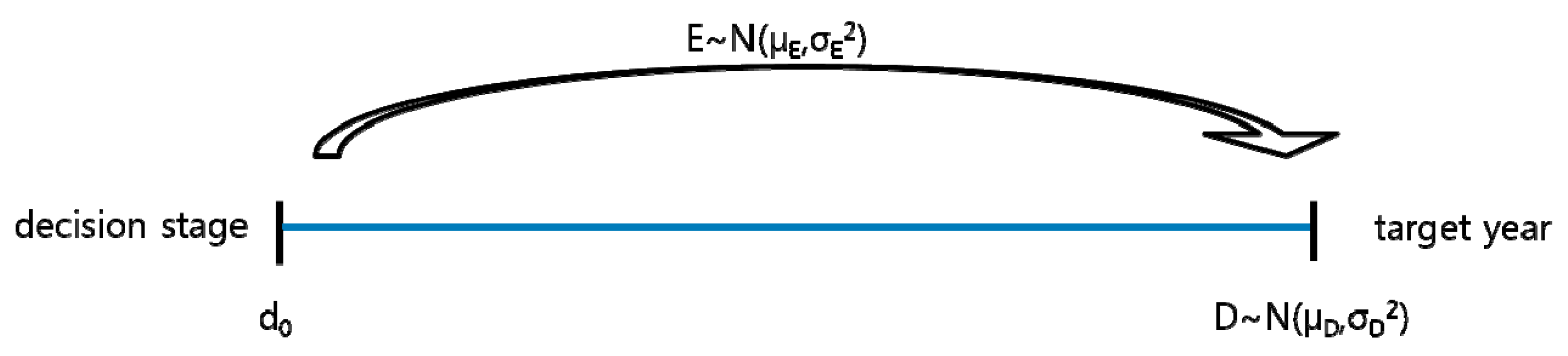
Predicted growth and the uncertainty of peak demand for the forecasting period are given by a random variable following a normal distribution as follows:
Given the current value of demand at the initial stage, the random variable of the peak demand at the target year also follows a normal distribution.
Here, is equal to and .
The two random variables in a single stage model are shown in Figure 2.
To represent the level of the forecasting uncertainty relevant to the expected peak demand, the relative standard deviation (RSD), also known as the coefficient of variation, is considered in percentage form as follows:
RSD is a standardized measure of dispersion of the probability distribution, and the value of RSD for a forecasting period is estimated from historical data. Given the estimated RSD value and the forecasted peak demand, the standard deviation can be calculated by rearranging Equation (3).
It is important to express the uncertainty as the ratio of the standard deviation to the expected demand rather than using the standard deviation alone because the value of demand may vary to a great extent over the planning horizon. Note that RSD is different from the mean absolute percentage deviation (MAPD), which is commonly used in the real world to represent the forecasting uncertainty in percentage form. For a normal probability distribution, MAPD is related to RSD as follows:
The value of uncertainty is estimated from historical data and can be expressed as a function of the forecasting period.
Equation (5) indicates that the extent of uncertainty depends on the forecasting period, regardless of the year in which forecasting is conducted.
For demand uncertainty in the proposed multi-stage model, a family of random variables for peak demand growth is formulated by the forecasting periods and years of the stages.
In (6), represents the expected demand growth from year for period and indicates the standard deviation. is calculated using Equation (3) with the values of and the forecasted peak demand for the year .
Then, a family of random variables for future peak demand is indexed by years.
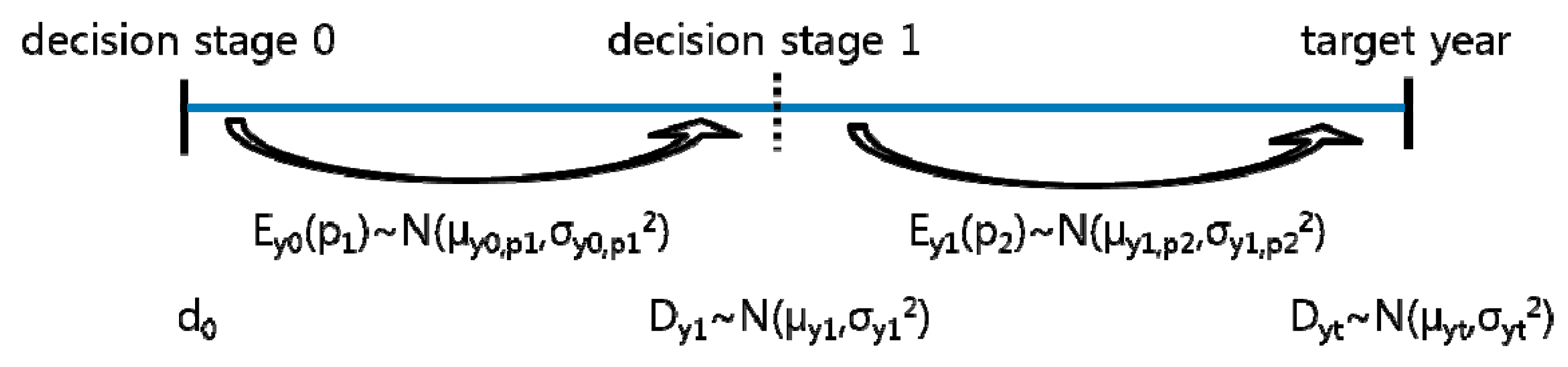
An example of a multi-stage model is shown in Figure 3. Here, is the peak demand random variable at year y1 forecasted at decision stage 0, and is the peak demand random variable at the target year forecasted at decision stage 1. The two random variables are given by
Note that if the peak demand of the target year is forecasted at the initial stage, the random variable may be different from in Equation (9) owing to the different forecasting periods for the two random variables.
As shown in Figure 3, the stochastic process involves independent increments; non-overlapping increments and are independent random variables when and for . The increments are random variables defined as . For non-overlapping forecasting periods, the random variables are independent because their parameters are independently determined. Based on the independent increment property, the values of expected peak demands are forecasted at the initial stage and are assumed to be fixed for the planning horizon. In the presented multi-stage model, there are middle stages where forecasting can be conducted again for the remaining years of the planning horizon, which may lead to newly forecasted peak demands. There is no possible way to foreknow the future forecasted values at the initial stage, but the level of the forecasting uncertainty can be estimated from historical data.
Under this condition, peak demands on the presented multi-stage model are expressed as the sum of a series of independent random variables. The succession of random steps by independent normally distributed random variables is represented as:
where is equal to , and .
Accordingly, the discrete-time stochastic process is a collection of random variables following normal distributions at all future stages.
2.3. TEP Problems with Multi-Stage Model
The uncertainty of the problem is not concerned with individual investment decisions, but with the optimal solution. In the presented framework, a TEP problem is solved for the network configuration of a target year. Thus, the last decision stage, where the optimal plan for the network configuration is completed, decides the overall uncertainty of the plan.
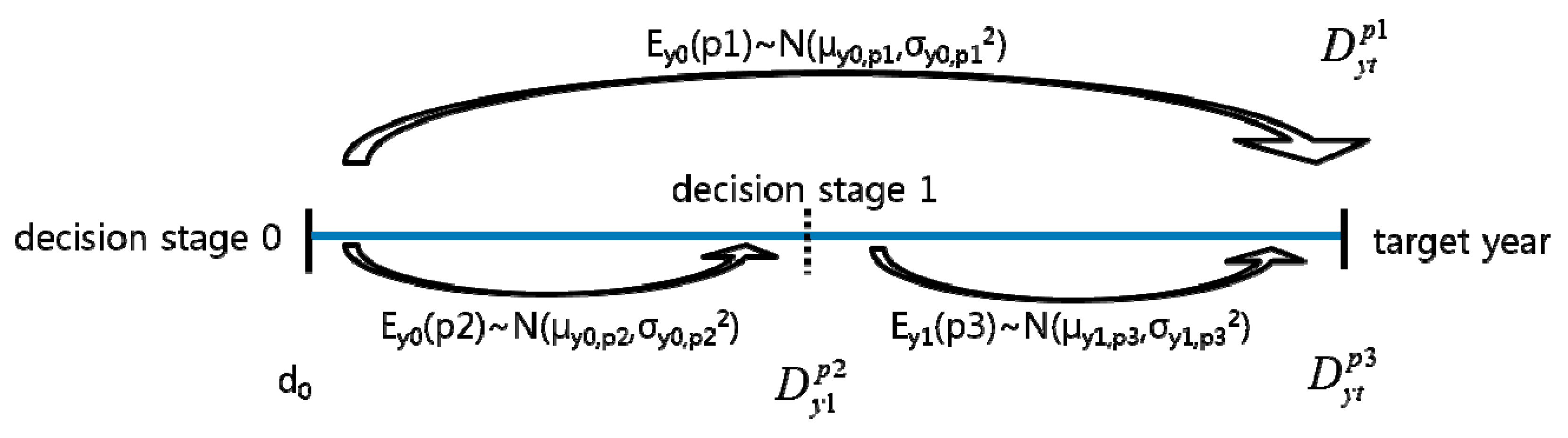
An example of the multi-stage model in a TEP problem is illustrated in Figure 4. is the peak demand random variable of the target year forecasted at decision stage 0, whereas is the peak demand random variable of the target year forecasted at decision stage 1. In this problem, investment options are assumed to have a lead time of either p1 or p3. Thus, there are two decision stages. For the sake of simplicity, three assumptions are used; , , and .
This problem may face different levels of uncertainty depending on the optimal solution. If the optimal plan of the TEP problem only consists of investment options with lead time p1, then the plan will face the uncertainty of . On the other hand, if the optimal plan includes an investment candidate with lead time p3, then the optimal decision will be completed at decision stage 1 and faces the uncertainty of . For each solution, the uncertainty level of the expected peak demand is computed as
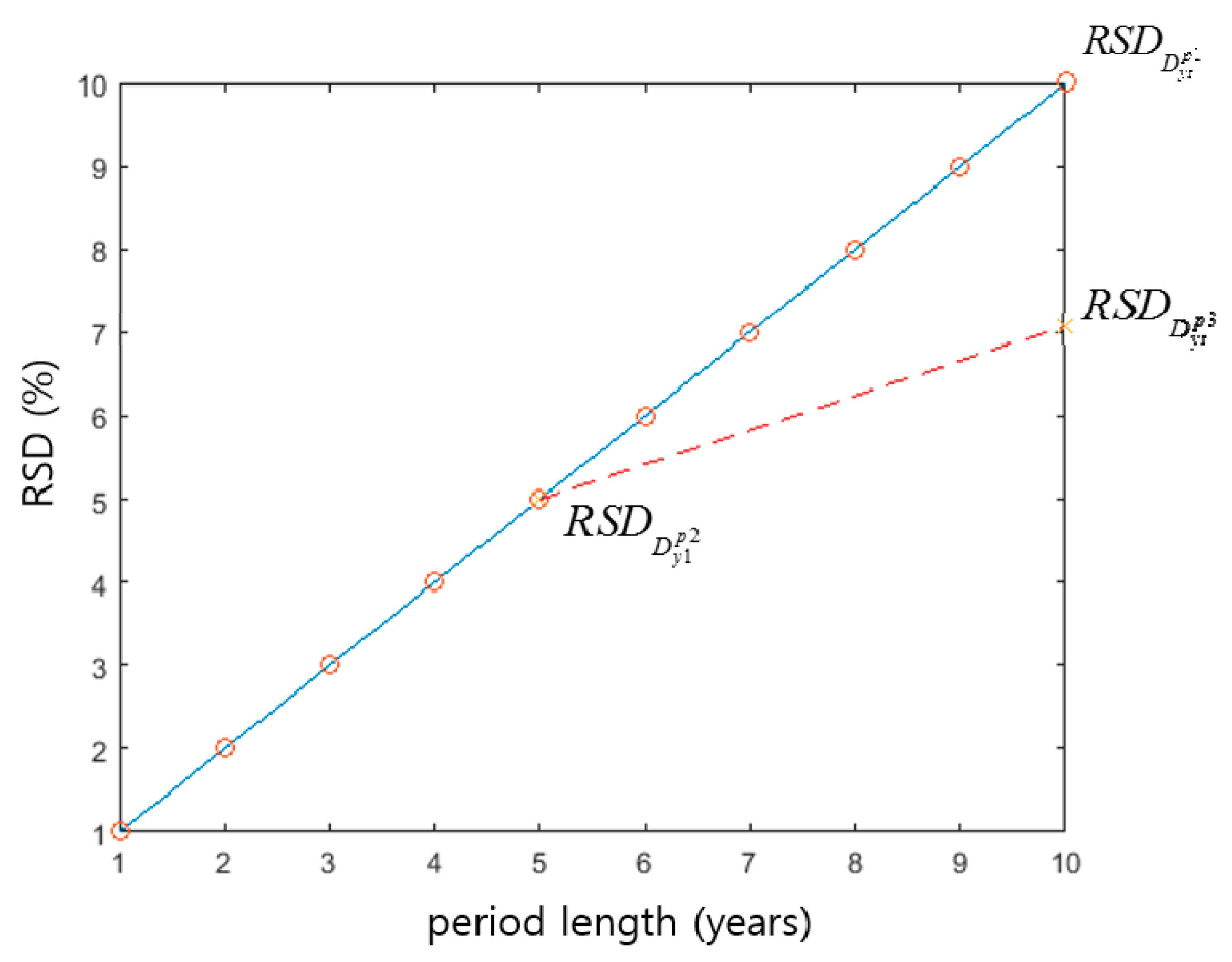
Here, is equal to because the forecasting period of the two stages is assumed to be equal. Because is equal to under the assumption of linearly increasing RSD, then is equal to Figure 5 depicts an estimated RSD curve and the RSD value of each solution. The RSD curve is a function of the forecasting period. Then, the RSD values are calculated based on the curve. Note that the value of depends on both the number of stages and the periods between stages. This method can be easily extended to general cases with varying expected demand growth, multiple stages with different periods, and any RSD curve estimated from historical data. In the proposed framework, the random variables of peak demand are modeled to follow normal distributions. Other probability distributions where stochastic approaches are applicable can be used in the proposed model.
3. Mathematical Formulation and Solution Procedure
3.1. Model Formulation
The typical formulation of TEP deterministic problems is given in Reference [32]. The objective is to minimize the sum of investment and load-shedding costs. To consider demand uncertainty, stochastic approaches are needed [5]. Then, the objective function is the sum of the investment cost and the expected load-shedding cost. The proposed framework is a stochastic problem. The formulation is modified to incorporate the proposed multi-stage model as follows:
subject to
The objective function in Equation (13) represents the sum of annualized investment costs and expected costs of generation and load shedding. The stochastic variable , which is the peak demand random variable of the target year, represents the uncertainty of the plan. The generation and load-shedding costs are dependent on the realization of the stochastic variable , whose parameters are determined by investment decisions. The objective function can be rewritten as the formulation of a stochastic programming application [33]:
Applying the general stochastic programming method to the problem requires specific parameters for .
In Equation (14), the constraint states the power balances at every node. The constraint in Equation (15) sets the limitation of maximum flow for each transmission line and the constraint in Equation (16) indicates a DC power flow model. The maximum capacity of the generators and the possible maximum load shedding value are stated in Equations (17) and (18), respectively. Equation (19) limits the phase angle between two nodes. Equation (20) means that is 1 for existing transmission lines and Equation (21) states that is a binary variable for investment candidates.
The mathematical model presented in Equations (13)–(21) is a mixed integer nonlinear problem owing to the constraint in Equation (16). The constraint can be replaced using a linear disjunctive model [34]:
where M is called a disjunctive parameter. Note that the constraint stated by Equation (23) is equivalent to Equation (16) when is equal to 1. Otherwise, the constraint becomes:
In Equation (24), the disjunctive parameter M must be large enough to avoid forcing a limit on the voltage angle difference between nodes and . When the value of M is too large, numerical instability may occur. The method for the appropriate selection of the disjunctive parameter is discussed in Reference [35].
3.2. Stochastic Mixed Integer Linear Problem
The formulation in Equations (13)–(21) is a stochastic problem in which the parameters of the stochastic variable are dependent on the decision variable . With a fixed set of parameters for the stochastic variable and the linearized constraint in Equation (23), the problem is formulated as a stochastic mixed integer linear problem, as follows:
subject to
In the objective function Equation (25), the set is a subset of and consists of investment options with lead times longer than or equal to . The constraint in Equation (34) ensures that at least one investment candidate with lead time is built. The uncertainty level of the planning problem is determined at the last decision stage where the network configuration of the target year is completed. Thus, the constraint in Equation (34) ensures a fixed set of parameters for the stochastic variable . The problem in Equations (25)–(34) finds the optimal solution among the investment candidates with lead times longer than or equal to under the uncertainty level determined by lead time . To find the optimal solution of the problem, all sets of parameters for the stochastic variable need to be considered. In the end, the problem in Equations (25)–(34) is repeatedly solved for all periods of lead times. Among the set of investment decisions, the solution with the minimum cost is the optimal plan.
Here, the forecasting period is equal to .
is a continuous random variable. To solve these problems, the variable must be discretized using Monte Carlo simulations and a sample average approximation. Then, the deterministic approximation of the stochastic problem can be obtained in the optimization model. Although the proposed framework is mathematically tractable, the optimization problem is combinatorial and stochastic. Applying the proposed method to large systems may require additional techniques such as scenario reduction.
3.3. Solution Procedure
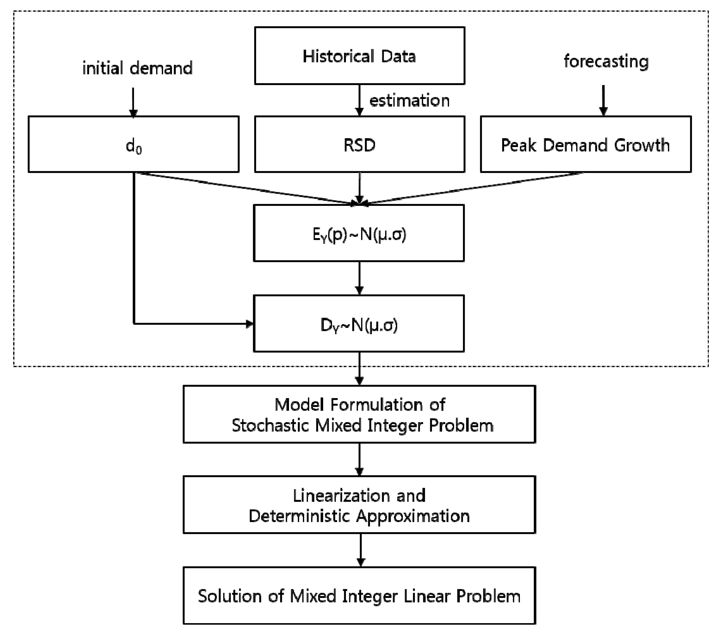
Figure 6 depicts the procedure followed by the proposed TEP framework. The dotted box shows the process of obtaining parameters and of the random variables and . Here, the value of RSD can be estimated from historical data, whereas the peak demand growth is forecasted for each year. With the obtained variables and parameters, the problem is formulated as a stochastic mixed integer problem. The solution method (mixed integer linear programming) is applied to the problem after linearization and deterministic approximation.
4. Case Studies
To verify the effectiveness of the proposed framework, case studies were conducted on a modified Garver’s six-bus system. The original data of Garver’s system is given in Reference [36] and more detailed data is given in Reference [32]. This system has been frequently used in TEP studies owing to the system’s capability to incorporate the characteristics of TEP problems. The stochastic problem was converted to a deterministic approximation by discretizing the continuous probability distribution representing the uncertainty of the peak demand. Monte Carlo simulations and a sampling average approximation were applied in the approximation. One thousand samples were used for each probability distribution in the sampling process. The parameter was set as 8760 because annualized costs were used throughout the case studies. Three simulations were implemented on the system to illustrate the proposed TEP framework. The first simulation examined the validity of the proposed framework. The second simulation showed the impact of RSD curve shapes in the proposed framework. The last simulation analyzed how different lead times influence the optimal solution of the proposed framework. The problems were solved in a general algebraic modeling system (GAMS). A computer with a 2.8 GHz processor and 4 GB RAM was used to conduct the simulations, and the average simulation time for the problems was 5 min.
4.1. Modified Garver’s Six-Bus System
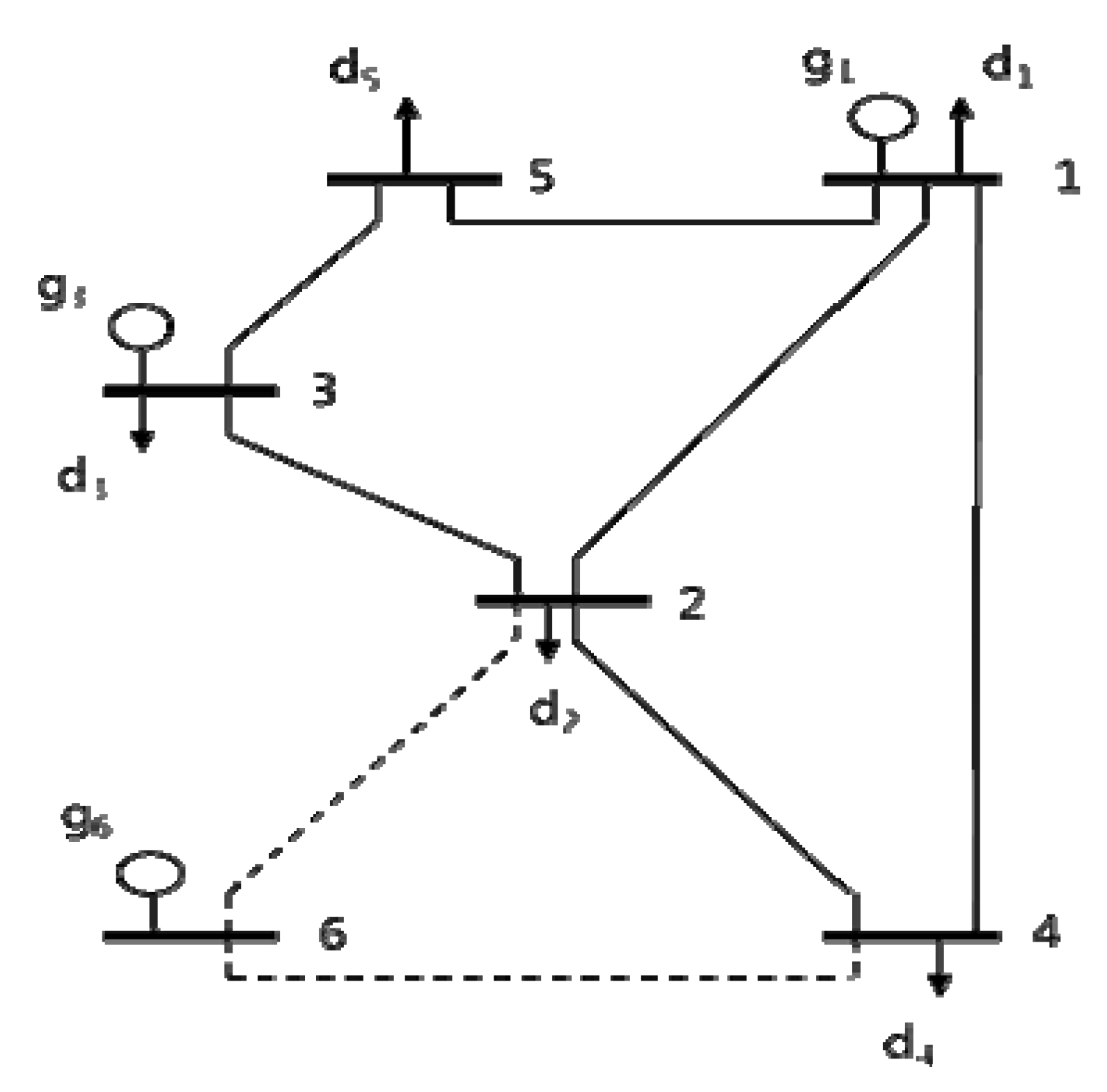
The configuration of Garver’s network is shown in Figure 7. The planning horizon was 10 years. The initial peak demand was 190 MW and annually increased by 4.94%, reaching 500 MW at the target year. The generation, load, and branch data are given in Table 1 and Table 2. The cost functions for the generating units were assumed to be linear, and initially six circuits exist in the system: 1–2, 1–4, 1–5, 2–3, 2–4, and 3–5. The existing six right-of-ways and two more right-of-ways (2–6, 4–6) were considered as new transmission investment candidates. Bus 6 was isolated in the initial configuration. Thus, the construction costs of transmission lines connecting to the bus and the associated construction lead times were assumed to be larger than the others, as shown in Table 2.
4.2. Simulation: Validity of the Proposed Framework
In this simulation, the validity of the proposed framework was examined. Three different models were used for the purpose: deterministic (Case 1), a stage model with a single lead time (Case 2), and the presented multi-stage model (Case 3). The first model represented deterministic approaches to solving TEP problems. In the simulation, a typical deterministic formulation was used, as given in Reference [32]. The second model represented conventional stochastic approaches with a single lead time. The last model was a stochastic approach with the proposed multi-stage model, which was capable of reflecting different lead times at different decision stages. The forecasting uncertainty was assumed to annually increase by 1.5%, reaching 15% in the final year of the planning horizon. The objective of each problem was to minimize the total expected cost. The simulation results are shown in Table 3 and Figure 8.
The cheapest generator was located at bus 6. Because bus 6 was isolated in the initial condition, L26 or L46 was/were constructed only when the benefit of cheap generation was greater than the cost of construction and load shedding. Moreover, the two transmission lines had a longer construction lead time than other transmission lines.
In Case 1, the total generation cost was not high enough to justify an investment to connect the cheap generating unit at bus 6. Thus, the optimal solution was to build two circuits in the existing right-of-ways and satisfy all demand with the generating units at buses 1 and 3. Although the investment cost was the least among the three cases, the solution was not prepared for the uncertainty of demand at all. Accordingly, under demand uncertainty, the generation cost was more expensive than in the other cases, which led to the highest total expected cost.
In Case 2, decisions were made only at the initial stage because the model assumed a single lead time for all investment candidates. Thus, the problem faced the forecasting uncertainty of a 10-year period. The optimal solution was to construct three circuits, two of which connected the generating unit at bus 6 to the initial system. The two circuits were more expensive than other solutions, but the relatively large uncertainty in peak demand may have led to a large amount of load shedding without them. The investment cost was the highest while the expected generation cost was the lowest in this case. The total expected cost of Case 2 was higher than that of Case 3 because Case 2 was exposed to a relatively large uncertainty.
In Case 3, the proposed approach was applied. The different lead times of investment candidates enabled the planner to make decisions at two stages: the initial year and the fifth year. The optimal solution was to build three circuits as in Case 2. However, the optimal network configuration was largely different. The optimal solution was completed at the second stage, when it was decided to build L23 and L35. Therefore, the optimal solution was exposed to less uncertainty than in Case 2. Only one circuit connecting the generating unit at bus 6 was built because circuit L46 was sufficient to cover the uncertainty in this case. The total expected cost was also the least in this case, indicating that the proposed approach showed better performance in dealing with the risk of uncertainty. Figure 9 shows an RSD curve estimated from historical data and the calculated RSD values. The value of was 10.6%, while the value of was 15%.
The results of the case studies yielded several implications. First, the proposed approach ensured that transmission network planners face less uncertainty than in conventional stochastic approaches with a single lead time. Second, considering lead times in the planning process may lead to a significant change in the optimal network configuration. This suggests that considering the lead times of investment candidates in the optimization process is important. Third, the case studies imply the importance of the RSD curve estimated from historical data and the lead times of investment candidates. In the simulation, the level of uncertainty was assumed to linearly increase every year. Then the RSD values were calculated based on the RSD curve. In the real world, the RSD curve can take any shape as long as it is an increasing function, and the lead times of investment candidates can be varied. The following simulations show the in-depth study of the proposed approach in terms of RSD curves and lead times.
4.3. Simulation: Various RSD Curve Shapes
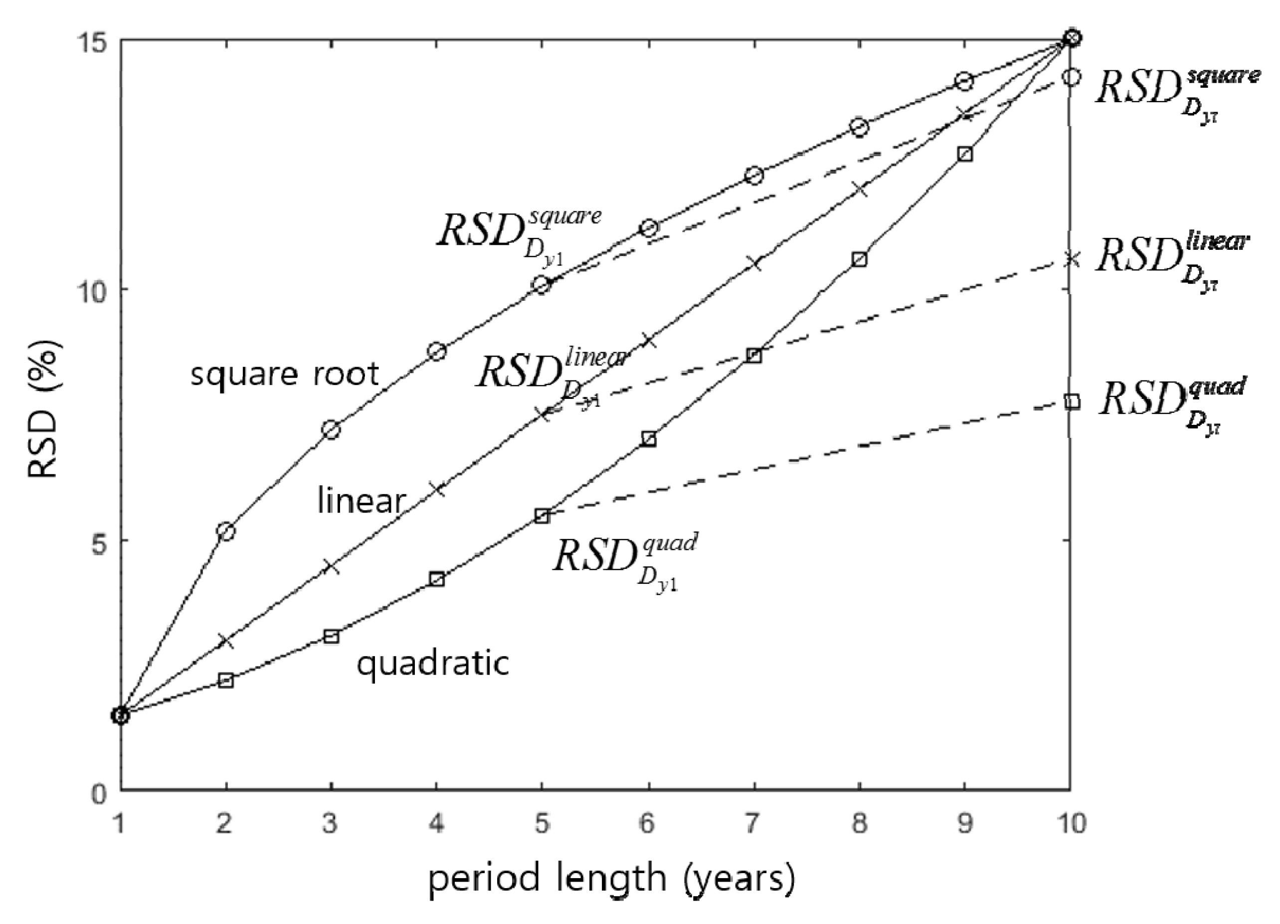
In this simulation, the impact of the RSD curve on the optimal solution was studied. Unlike the assumption of a linearly increasing RSD curve in the previous simulation, the uncertainty curve estimated from historical data can be any of various increasing functions in the real world. Three shapes were compared: linear, square root, and quadratic. The proposed approach was applied to all three cases. The curve shapes are shown in Figure 10, and the simulation results are provided in Table 4.
Compared to the linear curve, the uncertainty level of the square root curve rapidly increased for the first few years. The level of forecasting uncertainty for a 5-year period was 10.1% and the forecasting uncertainty at the second stage () was 14.3%. Even though the problem of the square root curve had a middle decision stage, the forecasting uncertainty at this stage was so large that the optimal solution was the same as that of the single-stage problem in Case 2. On the other hand, a quadratic RSD curve slowly increased for the first few years. Compared to the linear curve, the value of in the quadratic curve was smaller. Thus, the total expected cost was less than the linear curve, although the optimal solution was the same as for the linear curve.
The results of this simulation yielded two implications. First, the three cases based on curve types using the proposed method all had a lower than the single stage approach in Case 2. The different lead times of investment candidates offered the planner the opportunity to face less uncertainty in the optimal solution. Second, the shape of the RSD curve estimated from historical data was crucial for assessing uncertainty in the presented multi-stage model. It should be noted that the degree of advantage of having multiple decision stages in the proposed framework was dependent on the shape of the RSD curve.
4.4. Simulation: Various Lead Times
Investment options for transmission planning may possess different characteristics: available technology, length, environmental impact, and right-of-way. These characteristics influence the lead times of the investment candidates. In this simulation, the effects of different lead times on the proposed approach were investigated. A linearly increasing RSD curve was assumed in the problem. Three different scenarios for lead times and the results of the scenarios are shown in Table 5 and Table 6, respectively.
S1 had the shortest lead time for construction of existing transmission lines. However, the level of uncertainty and the total expected cost were the highest among the three scenarios. Although the lead times of the transmission lines were short, the demand at the time step of the last decision stage already included a large uncertainty. Thus, the result indicated that the level of uncertainty depended on not only the periods of the lead times but also on the time steps of the decision stages. S2 and S3 produced the same optimal solution. However, the uncertainty of S2 was slightly higher than that of S3 owing to the time step of the last decision stage. The three scenarios demonstrated that both the lead times of investment candidates and the time steps of decision stages were important in the proposed framework.
5. Conclusions
In this paper, we proposed a TEP framework with a multi-stage model under an uncertain environment. The framework considered transmission investment options for diverse lead times. In the presented multi-stage model, decision stages were determined by the diverse lead times of planning candidates. The level of uncertainty was represented using a relative standard deviation, and the uncertainty in the multi-stage model was studied. The proposed approach was formulated as a stochastic mixed integer linear problem. Mixed integer linear programming and stochastic programming were used in solving the optimization problem. Simulations were conducted on the modified Garver’s six-bus system. The results showed how the investment candidates involving various lead times affected the optimal decision under an uncertain environment. The proposed method achieved better performance than other methods in dealing with the risk of uncertainty. The shape of an RSD curve and the lead times of investment candidates were also shown to play a crucial role for evaluating uncertainty in the multi-stage model. The proposed method was mathematically tractable, but the combinatorial and stochastic problem required additional techniques for its application to large systems. Based on these results, the proposed framework was capable of incorporating any transmission investment options involving the addition of transmission capacity to deal with the risk of uncertainty. Transmission network planners can utilize the framework in the integrated planning of various technologies and lead times.
Author Contributions
All authors contributed to this work. W.W. designed the study, performed the analysis, and wrote the first draft of the paper. J.K. contributed to the conceptual approach and thoroughly revised the paper. Y.T. advised on mathematical formulations and supported the background research. M.K. provided important comments on modeling and analysis, and coordinated the proposed approach in the manuscript.
Acknowledgments
This research was supported by the Basic Science Research Program through the National Research Foundation of Korea (NRF) funded by the Ministry of Education (2017R1D1A1B03029308). This research was also supported by Korea Electric Power Corporation (grant number: R18XA06-75).
Conflicts of Interest
The authors declare no conflicts of interest.
Nomenclature
| Indices | |
| Years | |
| Transmission lines | |
| Demands | |
| Nodes | |
| Generating Units | |
| Forecasting periods, i.e., lead times | |
| Sets | |
| Years of stages | |
| Nodes | |
| Generating units | |
| Demands | |
| Transmission lines | |
| Forecasting periods, i.e., lead times | |
| Transmission investment candidates with lead time | |
| Transmission investment candidates with a lead time longer than or equal to | |
| Transmission line candidates | |
| Demands located at node | |
| Generating units located at node | |
| Sending-end node of Transmission line | |
| Receiving-end node of Transmission line | |
| Parameters | |
| Expected demand growth | |
| Standard deviation of | |
| Expected demand | |
| Standard deviation of | |
| Annualized investment cost of transmission line ($/MW) | |
| Discount rate | |
| Dimension factor | |
| Beginning year of the planning process | |
| Terminal year of the planning process | |
| Generation cost of generating unit ($) | |
| Load shedding cost ($) | |
| Susceptance of transmission line (S) | |
| Maximum transmission capacity of line (MW) | |
| Maximum generation capacity of unit (MW) | |
| Upper bound of load shedding for demand (MW) | |
| Binary Variable | |
| Binary variable that is 1 for the construction of transmission line , 0 otherwise | |
| Continuous Variables | |
| Power produced by generating unit (MW) | |
| Load shedding of demand (MW) | |
| Power flow through transmission line (MW) | |
| Voltage phase angle at node (rad) | |
| Stochastic Variables | |
| Stochastic variable for peak demand | |
| Stochastic variable for node demand | |
References
- Li, J.; Ma, Y.; Mu, G.; Feng, X.; Yan, G.; Guo, G.; Zhang, T. Optimal configuration of energy storage system coordinating wind turbine to participate power system primary frequency regulation. Energies 2018, 11, 1396. [Google Scholar] [CrossRef]
- Oprea, S.-V.; Bara, A.; Majstrovic, G. Aspects referring wind energy integration from the power system point of view in the region of southeast Europe. Study case of Romania. Energies 2018, 11, 251. [Google Scholar] [CrossRef]
- Fang, X.; Krishnan, V.; Hodge, B.M. Strategic offering for wind power producers considering energy and flexible ramping products. Energies 2018, 11, 1239. [Google Scholar] [CrossRef]
- Jo, K.H.; Kim, M.K. Improved genetic algorithm-based unit commitment considering uncertainty integration method. Energies 2018, 11, 1387. [Google Scholar] [CrossRef]
- Orfanos, G.A.; Georgilakis, P.S.; Hatziargyriou, N.D. Transmission expansion planning of systems with increasing wind power integration. IEEE Trans. Power Syst. 2013, 28, 1355–1362. [Google Scholar] [CrossRef]
- Choi, J.; Tran, T.; El-Keib, A.A.; Thomas, R.; Oh, H.; Billinton, A. A method for transmission system expansion planning considering probabilistic reliability criteria. IEEE Trans. Power Syst. 2005, 20, 1606–1615. [Google Scholar] [CrossRef]
- Choi, J.; Mount, T.M.; Thomas, R.J. Transmission expansion planning using contingency criteria. IEEE Trans. Power Syst. 2007, 22, 2249–2261. [Google Scholar] [CrossRef]
- Moreira, A.; Street, A.; Arroyo, J.M. An adjustable robust optimization approach for contingency-constrained transmission expansion planning. IEEE Trans. Power Syst. 2015, 30, 2013–2022. [Google Scholar] [CrossRef]
- Yu, H.; Chung, C.Y.; Wong, K.P.; Zhang, J.H. A chance constrained transmission network expansion planning method with consideration of load and wind farm uncertainties. IEEE Trans. Power Syst. 2009, 24, 1568–1576. [Google Scholar] [CrossRef]
- Teh, J.; Lai, C.M.; Cheng, Y.H. Composite reliability evaluation for transmission network planning. AIMS Energy 2018, 6, 170–186. [Google Scholar] [CrossRef]
- Hemmati, R.; hooshmand, R.A.; Kodabakhshian, A. State-of-the-art of transmission expansion planning: Comprehensive review. Renew. Sustain. Ener. Rev. 2013, 23, 312–319. [Google Scholar] [CrossRef]
- Lee, C.W.; Ng, S.K.; Zhong, J.; Wu, F.F. Transmission expansion planning from past to future. In Proceedings of the 2006 IEEE PES Power Systems Conference and Exposition, Atlanta, GA, USA, 29 Octomber–1 November 2006. [Google Scholar]
- Vinasco, G.; Rider, M.J.; Romero, R. A strategy to solve multistage transmission expansion planning problem. IEEE Trans. Power Syst. 2011, 26, 2574–2576. [Google Scholar] [CrossRef]
- Escobar, A.H.; Gallego, R.A.; Romero, R. Multistage and coordinated planning of the expansion of transmission systems. IEEE Trans. Power Syst. 2004, 19, 735–744. [Google Scholar] [CrossRef]
- Olsina, F.; Garcés, F.; Haubrich, H.J. Modeling long-term dynamics of electricity markets. Energy Policy 2006, 34, 1411–1433. [Google Scholar] [CrossRef]
- Newham, N. Power System Investment Planning Using Stochastic Dual Dynamic Programming. Ph.D. Thesis, University of Canterbury, Christchurch, New Zealand, April 2008. [Google Scholar]
- Lumbreras, S.; Ramos, A. The new challenges to transmission expansion planning. Survey of recent practice and literature review. Electr. Power Syst. Res. 2016, 134, 19–29. [Google Scholar] [CrossRef]
- Rabih, J. Robust Transmission network expansion planning with uncertain renewable generation and load. IEEE Trans. Power Syst. 2013, 28, 4558–4567. [Google Scholar]
- Silva, I.J.; Rider, M.J.; Romero, R.; Murari, C.A.F. Transmission network expansion planning considering uncertainty in demand. IEEE Trans. Power Syst. 2006, 21, 1565–1573. [Google Scholar] [CrossRef]
- Botterud, A.; Ilic, M.D.; Wangensteen, I. Optimal investments in power generation under centralized and decentralized decision making. IEEE Trans. Power Syst. 2005, 20, 254–263. [Google Scholar] [CrossRef]
- Roh, J.H.; Shahidehpour, M.; Wu, L. Market-based generation and transmission planning with uncertainties. IEEE Trans. Power Syst. 2009, 24, 1587–1598. [Google Scholar]
- Zhao, J.H.; Dong, Z.Y.; Lindsay, P.; Wong, K.P. Flexible Transmission expansion planning with uncertainties in an electricity market. IEEE Trans. Power Syst. 2009, 24, 479–488. [Google Scholar] [CrossRef]
- Yang, N.; Wen, F. A chance constrained programming approach to transmission system expansion planning. Elec. Power Syst. Res. 2005, 75, 171–177. [Google Scholar] [CrossRef]
- Botterud, A.; Korpas, M. A stochastic dynamic model for optimal timing of investments in new generation capacity in restructured power systems. Electr. Power Energy Syst. 2007, 29, 163–174. [Google Scholar] [CrossRef]
- Kagiannas, A.G.; Askounis, D.T.; Psarras, J. Power generation planning: A survey from monopoly to competition. Electr. Power Energy Syst. 2004, 26, 413–421. [Google Scholar] [CrossRef]
- Wu, F.F.; Zheng, F.L.; Wen, F.S. Transmission investment and expansion planning in a restructured electricity market. Energy 2006, 31, 954–966. [Google Scholar] [CrossRef]
- TYNDP 2018 Scenario Report. Available online: https://docstore.entsoe.eu/Documents/TYNDP%20documents/14475_ENTSO_ScenarioReport_Main.pdf (accessed on 1 September 2018).
- PJM Regional Transmission Planning Process. Available online: https://pjm.com/-/media/documents/manuals/archive/m14b/m14bv39-regional-transmission-planning-process-09-29-2017.ashx (accessed on 1 September 2018).
- Blanco, G.; Olsina, F.; Garcés, F.; Rehtanz, C. Real option valuation of FACTS investments based on the least square Monte Carlo method. IEEE Trans. Power Syst. 2011, 26, 1389–1398. [Google Scholar] [CrossRef]
- Konstantelos, I.; Strbac, G. Valuation of flexible transmission investment options under uncertainty. IEEE Trans. Power Syst. 2015, 30, 1047–1055. [Google Scholar] [CrossRef]
- Li, J.; Li, Z.; Liu, F.; Ye, H.; Zhang, X.; Mei, S.; Chang, N. Robust coordinated transmission and generation expansion planning considering ramping requirements and construction periods. IEEE Trans. Power Syst. 2018, 33, 268–280. [Google Scholar] [CrossRef]
- Romero, R.; Monticelli, A.; Garcia, A.; Haffner, S. Test systems and mathematical models for transmission network expansion planning. IEEE Proc.-Gener. Transm. Distrib. 2002, 149, 27–36. [Google Scholar] [CrossRef]
- Birge, J.R.; Louveaux, F. Introduction to Stochastic Programming; Springer: New York, NY, USA, 1997. [Google Scholar]
- Villasana, R.; Garver, L.L.; Salon, S.J. Transmission network planning using linear programming. IEEE Trans. Power Apparatus Syst. 1985, PAS-104, 349–356. [Google Scholar] [CrossRef]
- Sharifnia, A.; Aashtiani, H.Z. Transmission network planning: A method for synthesis of minimum-cost secure networks. IEEE Trans. Power Apparatus Syst. 1985, PAS-104, 2026–2034. [Google Scholar] [CrossRef]
- Garver, L.L. Transmission network estimation using linear programming. IEEE Trans. Power Apparatus Syst. 1970, PAS-89, 1688–1697. [Google Scholar] [CrossRef]
Figure 1.
Comparison of stage models in TEP.

Figure 2.
Single stage model with demand uncertainty.

Figure 3.
Demand uncertainty in multi-stage model.

Figure 4.
Example of multi-stage model in a TEP problem.

Figure 5.
Estimated RSD curve and calculated RSD values.

Figure 6.
Solution procedure–proposed TEP method.

Figure 7.
Initial configuration of Garver’s six-bus system.

Figure 8.
Simulation results for three different approaches.
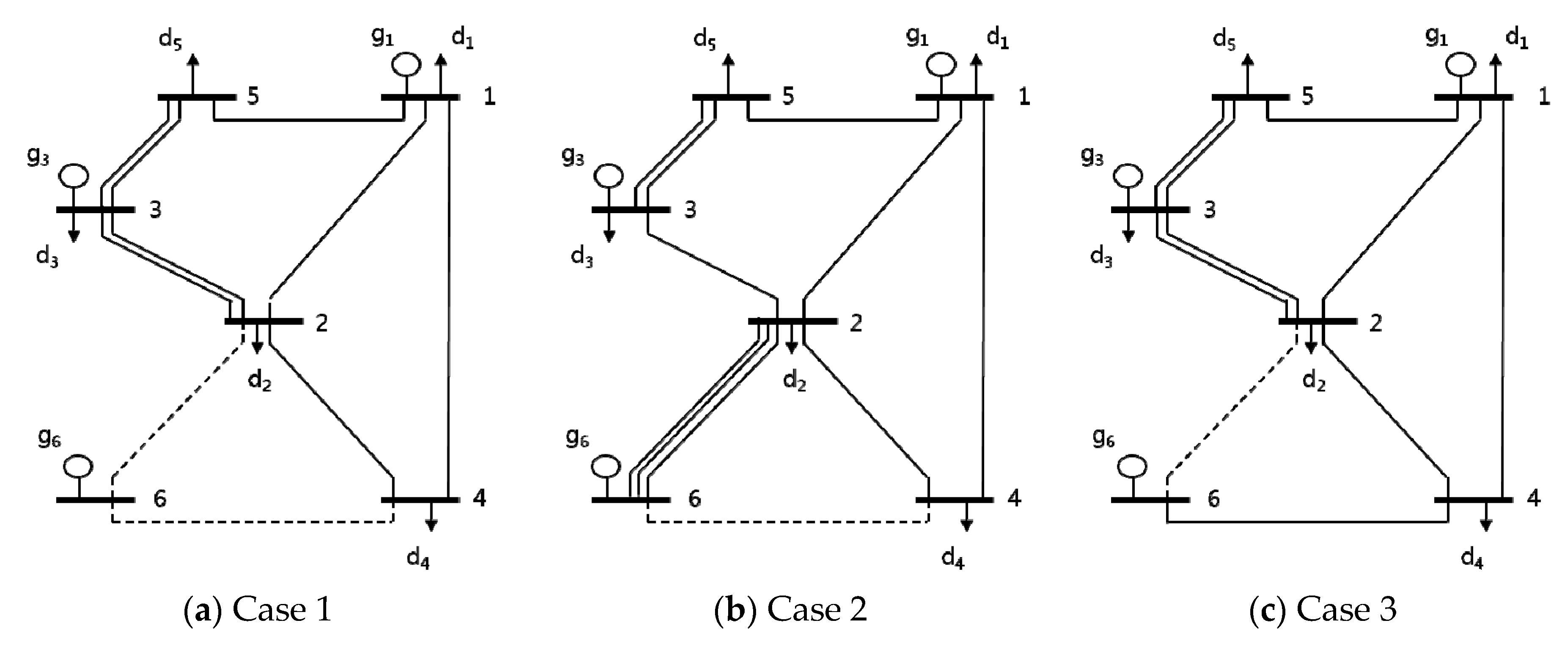
Figure 9.
Estimated RSD curve and calculated RSD values.
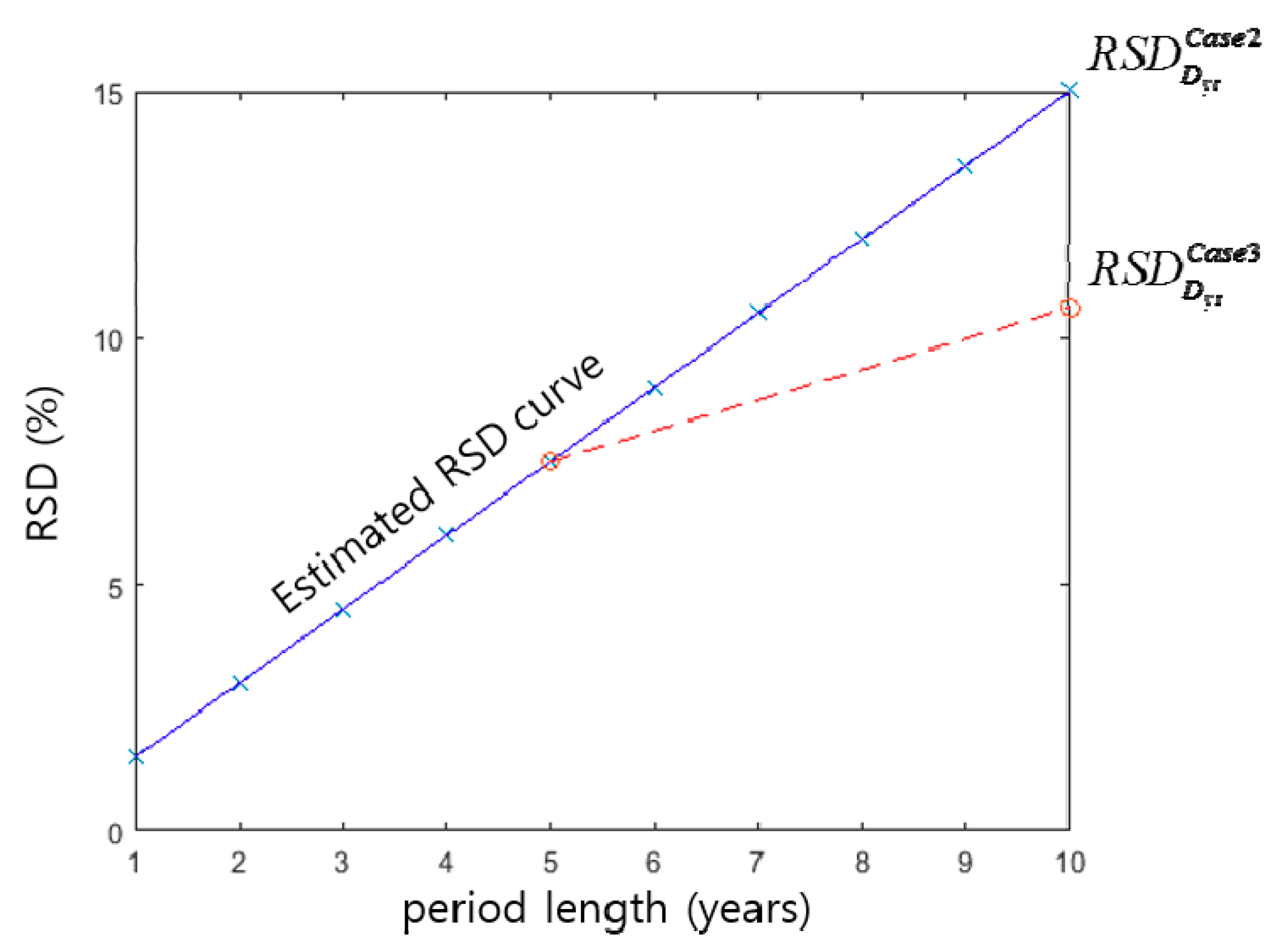
Figure 10.
Various shapes of RSD curves.


Table 1.
Generation and load data.
| Bus No. | Max. Generation (MW) | Generation Cost ($/MW) | Load (MW) | Load Shedding Cost ($/MW) |
|---|---|---|---|---|
| 1 | 150 | 21 | 80 | 150 |
| 2 | 0 | 0 | 240 | 150 |
| 3 | 360 | 17 | 40 | 150 |
| 4 | 0 | 0 | 160 | 150 |
| 5 | 0 | 0 | 240 | 150 |
| 6 | 600 | 10 | 0 | 150 |
Table 2.
Branch data.
| From–To | Lead Time (year) | Susceptance (S) | Cost (105$) | |
|---|---|---|---|---|
| 1–2 | 5 | 250 | 100 | 10 |
| 1–4 | 5 | 167 | 80 | 10 |
| 1–5 | 5 | 500 | 100 | 10 |
| 2–3 | 5 | 500 | 100 | 10 |
| 2–4 | 5 | 250 | 100 | 10 |
| 2–6 | 10 | 333 | 100 | 20 |
| 3–5 | 5 | 500 | 100 | 10 |
| 4–6 | 10 | 333 | 100 | 20 |
Table 3.
Results for different approaches.
| Case | Added Circuits | Investment Cost (105$) | Total Expected Cost (105$) | |||
|---|---|---|---|---|---|---|
| L23 | L35 | L26 | L46 | |||
| 1 | 1 | 1 | 0 | 0 | 20 | 863 |
| 2 | 0 | 1 | 2 | 0 | 50 | 854 |
| 3 | 1 | 1 | 0 | 1 | 40 | 839 |
Table 4.
Results for various RSD curves.
| Type | Added Circuits | |||||
|---|---|---|---|---|---|---|
| L23 | L35 | L26 | L46 | |||
| Linear | 1 | 1 | 0 | 1 | 7.5 | 10.6 |
| Square Root | 0 | 1 | 2 | 0 | 10.1 | 14.3 |
| Quadratic | 1 | 1 | 0 | 1 | 5.5 | 7.8 |
Table 5.
Different lead times of investment candidates.
| From-To | 1–2, 1–4, 1–5, 2–3, 2–4, 3–5 | 2–6, 4–6 | |
| Lead Time (year) | Scenario 1 | 1 | 10 |
| Scenario 2 | 3 | 10 | |
| Scenario 3 | 5 | 10 | |
Table 6.
Results for three scenarios.
| Scenario | Added Circuits | Total Expected Cost (105$) | ||||
| L23 | L35 | L26 | L46 | |||
| S1 | 0 | 1 | 2 | 0 | 13.6 | 851 |
| S2 | 1 | 1 | 0 | 1 | 11.4 | 841 |
| S3 | 1 | 1 | 0 | 1 | 10.6 | 839 |
© 2018 by the authors. Licensee MDPI, Basel, Switzerland. This article is an open access article distributed under the terms and conditions of the Creative Commons Attribution (CC BY) license (http://creativecommons.org/licenses/by/4.0/).
Share and Cite
MDPI and ACS Style
Kim, W.-W.; Park, J.-K.; Yoon, Y.-T.; Kim, M.-K. Transmission Expansion Planning under Uncertainty for Investment Options with Various Lead-Times. Energies 2018, 11, 2429. https://doi.org/10.3390/en11092429
AMA Style
Kim W-W, Park J-K, Yoon Y-T, Kim M-K. Transmission Expansion Planning under Uncertainty for Investment Options with Various Lead-Times. Energies. 2018; 11(9):2429. https://doi.org/10.3390/en11092429
Chicago/Turabian StyleKim, Wook-Won, Jong-Keun Park, Yong-Tae Yoon, and Mun-Kyeom Kim. 2018. "Transmission Expansion Planning under Uncertainty for Investment Options with Various Lead-Times" Energies 11, no. 9: 2429. https://doi.org/10.3390/en11092429
Note that from the first issue of 2016, this journal uses article numbers instead of page numbers. See further details here.