Investigations on the Developed Full Frequency- Dependent Cable Model for Calculations of Fast Transients †

1
Department of Electrical Engineering and Information Technology, Chemnitz University of Technology, 09128 Chemnitz, Germany
2
Department of Electrical Engineering and Informatics, University of Applied Sciences Zittau/Goerlitz, 02763 Zittau, Germany
*
Author to whom correspondence should be addressed.
†
This paper is an extended version of our paper published in Hoshmeh, A.; Malekian, K.; Schuftt, W.; Schmidt, U. A single-phase cable model based on lumped-parameters for transient calculations in the time domain. In Proceedings of the 2015 IEEE 15th International Conference on Environment and Electrical Engineering (EEEIC), Rome, Italy, 10–13 June 2015
Energies 2018, 11(9), 2390; https://doi.org/10.3390/en11092390
Submission received: 27 June 2018
/
Revised: 5 September 2018
/
Accepted: 6 September 2018
/
Published: 11 September 2018
(This article belongs to the Section F: Electrical Engineering)
Abstract
:The knowledge about the behavior of cables is substantial in cases of transients or in cases of faults. However, there are only a few models that are tailored to the current requirements for calculations of transient phenomena in three-phase cable systems. These models are based on complex structures. PI-section cable models with simple structures were previously qualified only for calculations in the frequency domain. A new full frequency-dependent cable model to simulate transient phenomena is introduced and validated. The model is based on lumped parameters with cascaded frequency-dependent PI-sections. For the implementation and the integration in simulation tools, it is important to investigate the impact of the PI-section parameters to the accuracy, the stability and the mathematical robustness. In this work, the impact of the frequency dependence of cable parameters, the length distribution and the number of PI-sections on the results of the developed three-phase cable model have been discussed. For simulations in the time domain, two algorithms have been presented to optimize the number of PI-sections based on a specified accuracy.
1. Introduction
Underground cables are an important part of electrical power systems in the HV, the EHV and the UHV level. Their application and the impact has increased with the growth of wind and solar energy to the total electricity generation [1,2]. The knowledge about the behavior in cases of transients is required for the correct design of cable lines and the overvoltage protection. The major difficulty for the modeling of cables is the complexity of the geometrical configuration and the electromagnetic coupling between phase conductors, cable shield and the earth. For this case, applicable models are required for the calculation of the electrical stresses. Effective models exist for load flow calculations and for calculations in the frequency domain. Older models were derived from approaches for overhead line calculations [3,4,5,6,7,8,9,10]. The results of these models have problems with result accuracy and the robustness. The incorrect modeling of geometrical condition and the incomplete interpretation of electromagnetic coupling are the reasons for the problems. To achieve a proper accuracy, a model with exact frequency-dependent cable parameters and with a good reproduction of wave propagation behavior is required.
In [11] a new full frequency-dependent three-phase PI-section cable model (3P-PI-Model) is introduced and validated. The frequency-dependent impedances in the model are determined with an improved sub-conductor method considering the skin and the proximity effect in the core, the shield and the earth [12,13]. The wave propagation in the model is based on PI-sections. The frequency dependence of the cable parameters is reproduced by means of vector fitting algorithm [14,15] and implemented through an RLC-network in a defined number of PI-sections. To decouple the three-phase cable system, a modal transformation is used [16,17,18].
For the implementation in calculation software, it is important to understand the behavior and the impact of the model parameter to the results. The significant problems of using PI-sections are their main resonance and the computational effort, which results from working with a large number of PI-sections. These problems can be influenced in the developed 3P-PI-Model through different parameters. The most important parameters, which have a direct impact, are the frequency dependence of cable parameters, length distribution of PI-sections and the number of PI-sections. To reduce the computational effort in the new model, two algorithms have been introduced for optimizing the number of PI-sections.
2. Wave Propagation Cable Model
The wave propagation in a multi-conductor cable or transmission line can be represented in the frequency domain with second-order differential Equations [19]:
The longitudinal impedances and the shunt admittance in the phase domain are calculated using the developed algorithms in [12,13]. The index “L” stands for lateral. In order to solve the differential Equations (1) and (2), a modal transformation technique has been proposed in [19]. As a result, the coupling between the cable conductors disappears and the cable system can be considered as decoupled single conductors. In the modal domain, Equations (1) and (2) can be rewritten as:
where is a diagonal matrix which represents the eigenvalues matrix of and . For the transformation into modal domain the modal transformation matrices and are used. The relation between the matrices is given in [20]:
Therefore, it is sufficient to calculate only one of them. In this paper, the results for will be calculated as in [17]. In order to perform the calculation in the modal domain, the quantities , , and have to be transformed into this domain. From Equations (3) and (4), it can be derived:
With simple matrix perturbation, the above equations are then rewritten as:
By rearranging the terms and by using the Equation (5) in (8) and (9), the longitudinal impedance and the shunt admittance in the modal domain can be defined as:
Both matrices in Equations (10) and (11) are diagonal. The frequency dependence of the elements of cannot be neglected (as assumed for the elements of ). This is related to the frequency dependent elements of . The elements of are also strong frequency dependent. In order to take the frequency dependency of and into account, their diagonal elements will be approximated by mathematical functions using the vector fitting algorithm (VF) [14,15]. For example, the first diagonal element in can be approximated using VF as:
The accuracy of depends on the number of the real terms N and the number of the complex terms M. can be reproduced with an electrical network. In [21], a RL-network has been used. Using such a network allows to employ only the real poles and residues in the approximation (the complex terms are discarded). Although the fitting is achieved with a low order of approximation, the accuracy is affected. In this paper, an RLC-network shown in Figure 1 is introduced to regard all the poles and residues in the approximation including the complex terms.
As can be seen, the network has been divided into two sections. The elements of the section I can be evaluated in a similar way as in [21]. The elements of section II are obtained as follows:
The first diagonal element of is similarly approximated. Furthermore, and are assumed to be zeros in . After calculating and , they will be combined to form a developed PI-section. Figure 2 shows a representation for the developed PI-section after regarding the cable length, where and are the voltages in the modal domain at sending and receiving end respectively. One single conductor in the developed cable model can then be represented by cascading a number of PI-sections. Basically, the number of PI-sections depends on the cable length.
For the remaining diagonal elements of and , the same procedure is used to form the other conductors in the developed cable model. From the Equations (3)–(5), the voltages and the currents are transformed into the modal domain as follows:
The Equations (14) and (15) are still in the frequency domain. However, since the simulations in the power system are necessary in the time domain, these equations have to be transformed into this domain. For the voltages in Equation (14), the convolution integral is applied as:
Evaluation of this integral point by point is time consuming. By approximating the elements of using rational functions, an efficient recursive convolution method is used [7] and the above integral can be rewritten as a sum of exponentials:
where b and l are the approximations parameters of the rational functions. The wave travel time for the impulse from one end of the cable to the other one is related to the imaginary term of the propagation function :
The voltage vector is calculated recursively from as:
In this relation, , and are constants that mainly depend on b, l and [19]. The same procedure is used to transform the currents in Equation (15) into the time domain. In order to execute the time domain simulations, the differential equations for single conductors in the developed cable model have to be formulated. As shown in [21], the differential equations can be represented using state space techniques. A numerical Backward Euler rule of integration can then be applied to find the solution for the related state space equations [22]. To solve the cable equations with the rest of the network, which is always defined in phase quantities, the calculated voltages and currents in the modal domain must be transformed back to phase quantities. Figure 3 shows an overview for the realization of the 3P-PI-Model.
Starting from defining and , the cable model part is executed only once to provide the PI-sections for the calculation part. In this part, the computation is evaluated every . For the first one, the vector of the voltages is calculated using the network model and the vector of the currents . By applying the recursive convolution between and the approximation of (), the vector of the voltages is calculated. Using the PI-sections and , the state space equations are formulated and solved by means of numerical Backward Euler rule of integration to yield the current vector . The recursive convolution between and the approximation of () provides the vector of currents for the next .
3. Analysis in the Frequency Domain
3.1. Impact of the Frequency Dependent Cable Parameters
Figure 4 shows a traditional PI-section without considering the frequency dependence of cable parameters for PI-section length of ℓ.
As it can be seen, the main elements are divided into longitudinal (R and L) and shunt (C and G) parameters. In the study, constant permittivities are assumed for the insulation and semiconducting layers. It makes the shunt capacitance also frequency independent. The frequency dependence of the conductance is negligible [23,24]. As shown in [12,13], the strong frequency dependence of the cable longitudinal parameters makes it necessary to regard this dependency to simulate transient phenomena.
Contrary to the traditional PI-Model, where the cable parameters are calculated at a certain frequency [25], the developed 3P-PI-Model includes the frequency dependence of the longitudinal impedance using an RLC-network (see Figure 1).
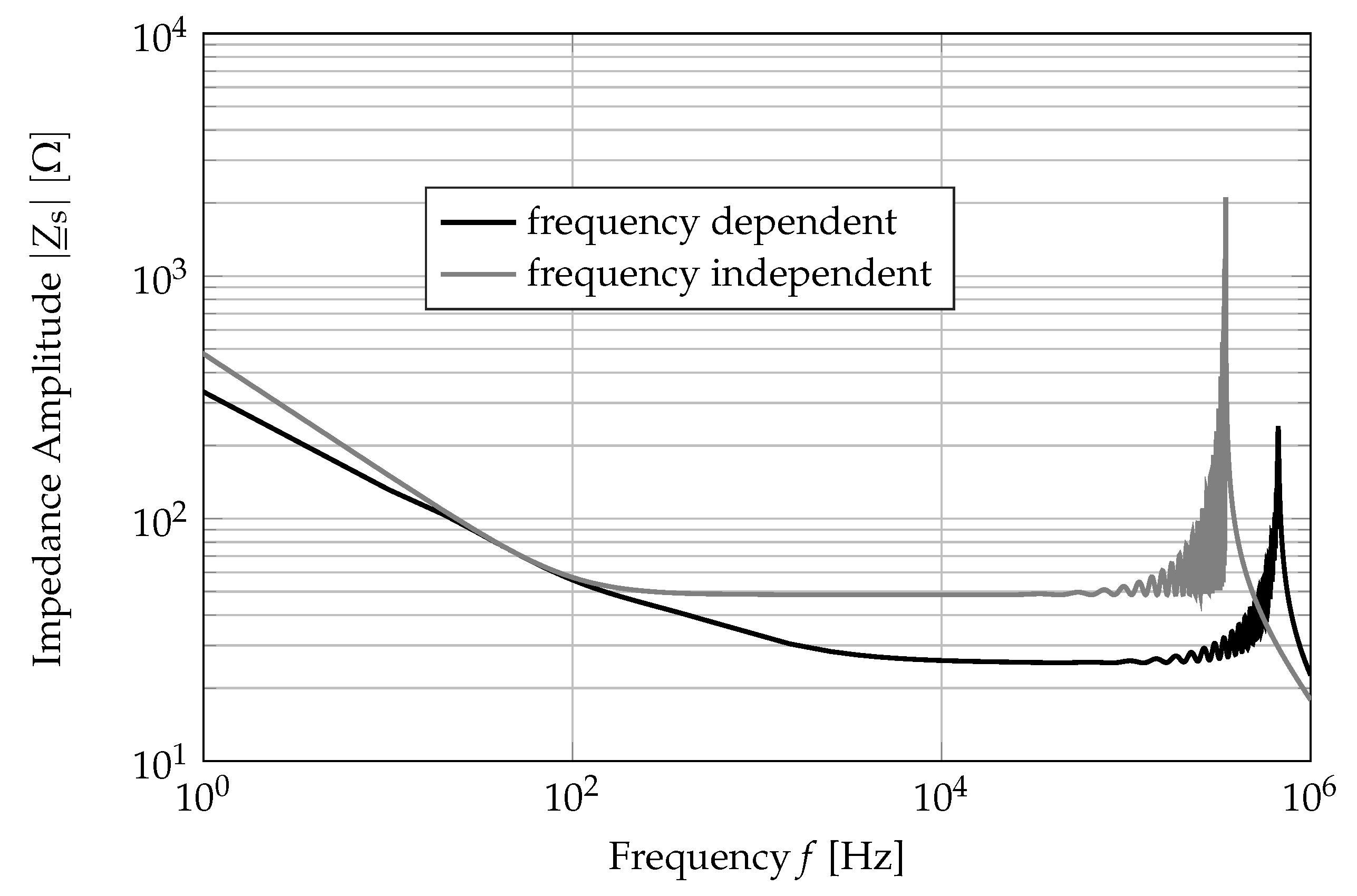
The importance of regarding the frequency dependence is well presented in Figure 5, where a comparison between the amplitude of the cable impedance at sending end with and without considering the frequency dependence of the longitudinal parameters is shown. The impedance response for both cases is calculated after connecting the receiving end of the cable to its characteristic impedance [25]. The cable type is given in Table 1.
The calculations for the case without regarding the frequency dependence of the longitudinal parameters (traditional PI-Model) are carried out using the cable parameters at 50 Hz. For the case with taking the frequency dependence of the longitudinal parameters into account (developed 3P-PI-Model), the parameters are calculated using the proposed algorithm in [12,13].
As it can be seen, the amplitude of both models matches only at 50 Hz. The resonances of all PI-sections in both models accumulate and form a main resonance. This main resonance can be excited and therefore produce unwanted oscillations in the time domain, which do not exist in reality. This fact is a main problem when applying the PI-sections. However, as shown in this figure, for the same number of the PI-sections, the main resonance of the developed model is milder than one in the traditional PI-section model. In this case, the amplitude of the main resonance is about 10 times lower. The damping at the frequency of the main resonance is higher in comparison with damping in 50 Hz [13]. Therefore, considering the frequency dependence leads to a lower amplitude of the main resonance and as a result, to smaller unwanted oscillations.
Another difference between the results shown in Figure 5 is the frequency of the main resonance. The higher frequency of the main resonance in the developed 3P-PI-Model can be explained with considering the frequency dependence and therefore having a lower inductance in comparison to the traditional PI-Model [13,26,27,28]. However, this fact does not directly have any considerable role in the results in the time domain. The first helpful effect here is that the main resonance is shifted thereby to a higher frequency with the higher damping. Secondly, a resonance at higher frequency is less likely to be excited during the calculations when the resonance is farther away from the frequency range of the simulated transients.
In sum, considering the frequency dependence can be a proper remedy for problems associated with applying the PI-sections.
3.2. Impact of the Length Distribution of PI-Sections
The accumulation of the individual resonance frequency of PI-sections leads to a main resonance (see Figure 5). This main resonance can be excited in the time domain, which will lead, depending on its amplitude, to unwanted oscillations. These oscillations can be influenced by distributing the length of PI-sections differently, which results in distribution profiles over the cable length ℓ.
The distribution profiles that give the best results are shown in Figure 6 for the cable length km and the number of PI-sections . The length of one PI-section is and its number is ( = 1 ... ).
In the case of uniform distribution, all PI-sections have the same length. In the parabola distribution, the length of each PI-section from the beginning to the middle of the cable is reduced. The section from the middle to the end of the cable is mirrored from the beginning to the middle of the cable. In the trapezoidal distribution, the first and last two PI-sections are shorter than the remaining PI-sections, which are evenly distributed.
The uniform distribution shown in Figure 6 is mainly used in the traditional PI-Model. Therefore, the impedance at the beginning of the cable when using the uniform distribution will be used as reference impedance in this section.
Figure 7 presents the amplitude of cable impedance for the distribution profiles shown in Figure 6. The calculations are carried out for the 3P-PI-Model after connecting the receiving end of the cable to its characteristic impedance. The cable length is km. The number of PI-sections is .
As it can be seen, the distribution profiles shown in Figure 6 lead to the same impedance up to a certain frequency. The distinguishing characteristics of the impedances only relate to the amplitude and the location of the main resonance. The use of the parabola distribution results in a smaller amplitude of the main resonance compared to the uniform distribution. However, the main resonance of the parabola distribution has a lower frequency. The amplitude of the main resonance of the trapezoidal distribution is greater than that of the uniform distribution. However, the location of its main resonance has the highest frequency. This comparison leads to the conclusion that the distribution profile of PI-sections have an impact on the amplitude and the frequency of their main resonance.
As a compromise between the high frequency and the low amplitude of the main resonance of PI-sections, the uniform distribution is used for subsequent calculations.
3.3. Impact of the Number of PI-Sections
For investigating the impact of the number of PI-sections on the 3P-PI-Model’s behavior, the distributed-parameters model, considering the frequency dependence of the cable parameters, is used as a reference. It should be noted that the reference model in the frequency domain can be developed without any simplifications. However, it is not directly applicable for the time domain calculations. To apply the reference model in these calculations, some simplifications are required [29,30,31].
For a single phase cable system, which is modeled through distributed-parameters, the current and voltage equations at the sending end are described as follows [19]:
where
According to Equations (20) and (21), if the receiving end of the cable is connected to the characteristic impedance, the cable impedance at the sending end will be the same as the characteristic impedance
Figure 8 shows the amplitude of the cable characteristic impedance for the distributed-parameters model and the developed 3P-PI-Model for different numbers of PI-sections.
As shown, for a specific cable length and depending on the number of PI-sections, the behavior of the developed 3P-PI-Model will agree with the distributed-parameters model over a certain frequency range. By increasing the number of PI-sections, this range will be expanded.
For simulation of transients in the time domain, a large number of PI-sections has to be used in order to get a good accuracy. However, increasing the number of PI-sections leads to higher computational effort. This is caused by the higher dimension of the differential equations. Therefore, an optimization of the number of PI-sections is needed.
4. Analysis in the Time Domain
For modeling of cables with PI-sections, a minimum number of these sections has to be used. The number of PI-section depends mainly on the cable length and the simulated event. The longer the cable is, the more PI-sections are needed. In addition, more PI-sections are needed to simulate transient events (e.g., lightning strikes or switching operations) compared to steady state operations (e.g., during normal operation or failure).
4.1. Optimization of the Number of PI-Sections—First Algorithm
For optimizing the number of PI-sections in the developed 3P-PI-Model, a DC-Test on a three-phase cable with a length of in trefoil formation has been used. The test is performed by charging the cable conductors up to 1 kV. After that, the charged conductors are connected to earth through the circuit breaker (s2) and the discharge current at the sending end is simulated. The test configuration is shown in Figure 9. The cable parameters are given in Table 1.
Figure 10 shows the discharge current with different number of PI-sections.
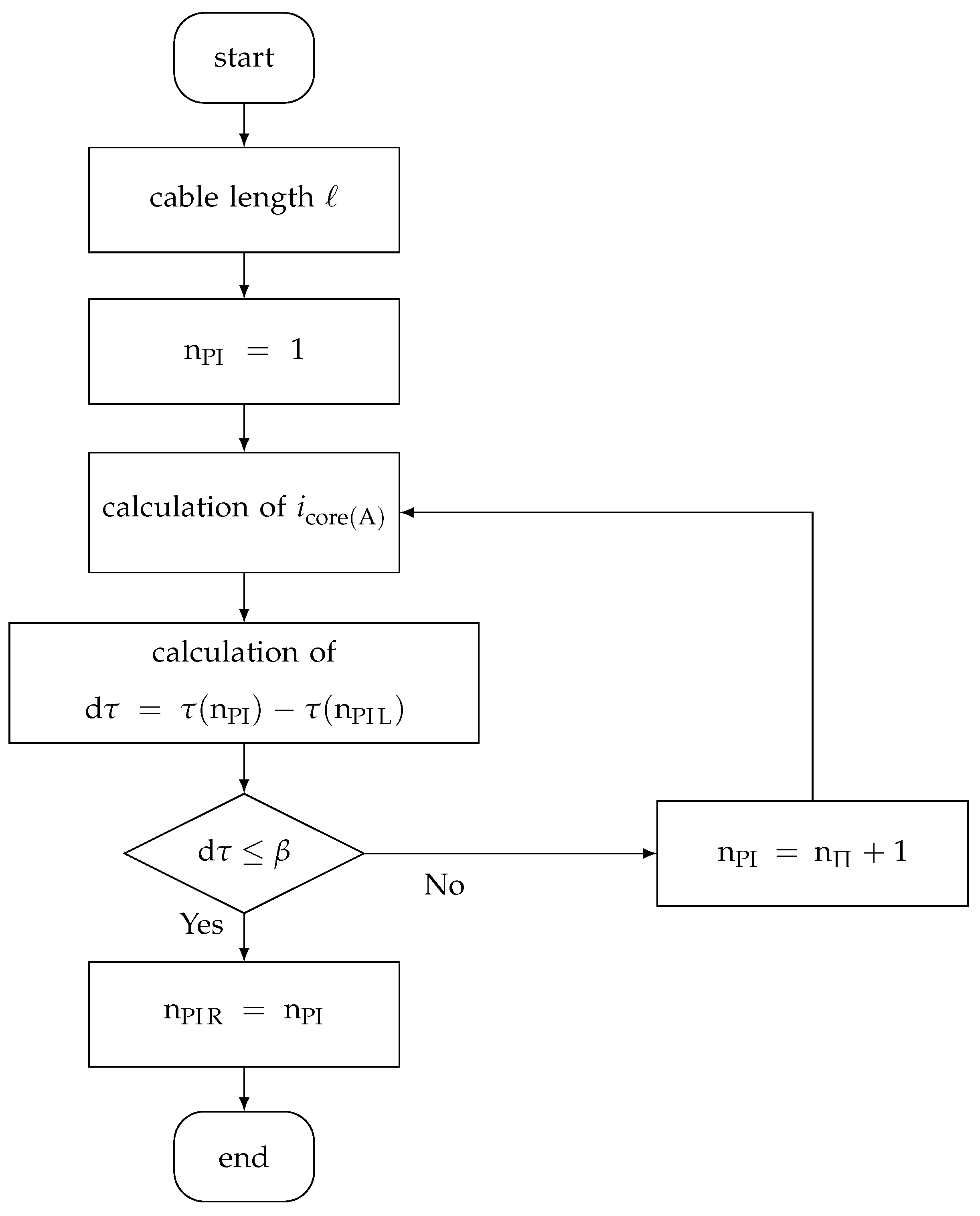
As it can be seen, the slope of the current increases and the time delay of the current decreases. This is mainly due to the better replication of the higher frequencies in the current by increasing the number of PI-sections. However, the change in time delay becomes smaller as the number of PI-sections increases. Above a certain number of PI-sections, this change can be neglected. Therefore, it is useful to set an upper limit on the number of PI-sections to optimize the computational effort. The upper limit of the number of PI-sections is determined using the algorithm shown in Figure 11.
For a given cable length ℓ, the number of PI-sections increases until the relative change in the time delay is less than a defined limit. The limit is initially set to . If the time delay is lower than this limit, then the loop is interrupted and the reached number of PI-sections is stored as the upper limit .
In this context, it should be noted that the overshoot of the current in Figure 10 (e.g., in the range s) is minimized and thus the amplitude of the current is also optimized by optimizing the time delay of the current. The reason is the dependence of the amplitude of the current on the characteristic impedance of the cable. This characteristic impedance is mainly calculated from the inductance and the capacitance of the cable, which in turn are included in the calculation of the time delay (see Equation (23)).
Figure 12 shows the upper limit of the number of PI-sections depending on the cable length in the range km.
For accurate simulation results, the number of PI-sections must be increased until the frequency of their main resonance is greater than the highest frequency of the event to be simulated. By increasing the cable length, the frequency of the main resonance of PI-sections will decrease [25]. In order to get the same accuracy of the calculations, the number of PI-sections has to be increased as it can be seen in Figure 12. For example, to simulate of transients by a cable length of 2.5 km the number of PI-sections is 45 and by a cable length of 10 km this number will increase to 52.
The proposed algorithm shown in Figure 11 defined the number of PI-sections in order to reach very good accuracy in the developed 3P-PI-Model, which results in using a large number of PI-sections. However, in many cases of simulation of transients a proper accuracy can be accepted. Therefore, the large number of PI-sections can be reduced and thus so can the computational effort.
4.2. Optimization of the Number of PI-Sections—Second Algorithm
The main idea of the second algorithm is to reduce the computational effort of the calculations in the developed 3P-PI-Model at the expense of the accuracy.
Figure 13 illustrates the methodology of the second algorithm for the example shown in Figure 9. In this algorithm, the number of PI-sections is reduced to such an extent that a given error in the time delay with respect to a reference value is not exceeded. The number of PI-sections will store under the reduced number . The reference value of the time delay is defined at upper limit by the number of PI-section , whereat the error in the time delay is equal to s.
By using the upper limit of the number of PI-sections shown in Figure 12 in the second algorithm the reduced number of PI-sections can be calculated for different errors in the time delay. Figure 14 shows the results for two specified errors.
As it can be seen, specifying an error in the time delay leads to a considerable reduction in the number of PI-sections compared to their upper limit. For example, by a cable length of 2.5 km the number of PI-sections decreases from 41 to 12 by s and to 4 by s.
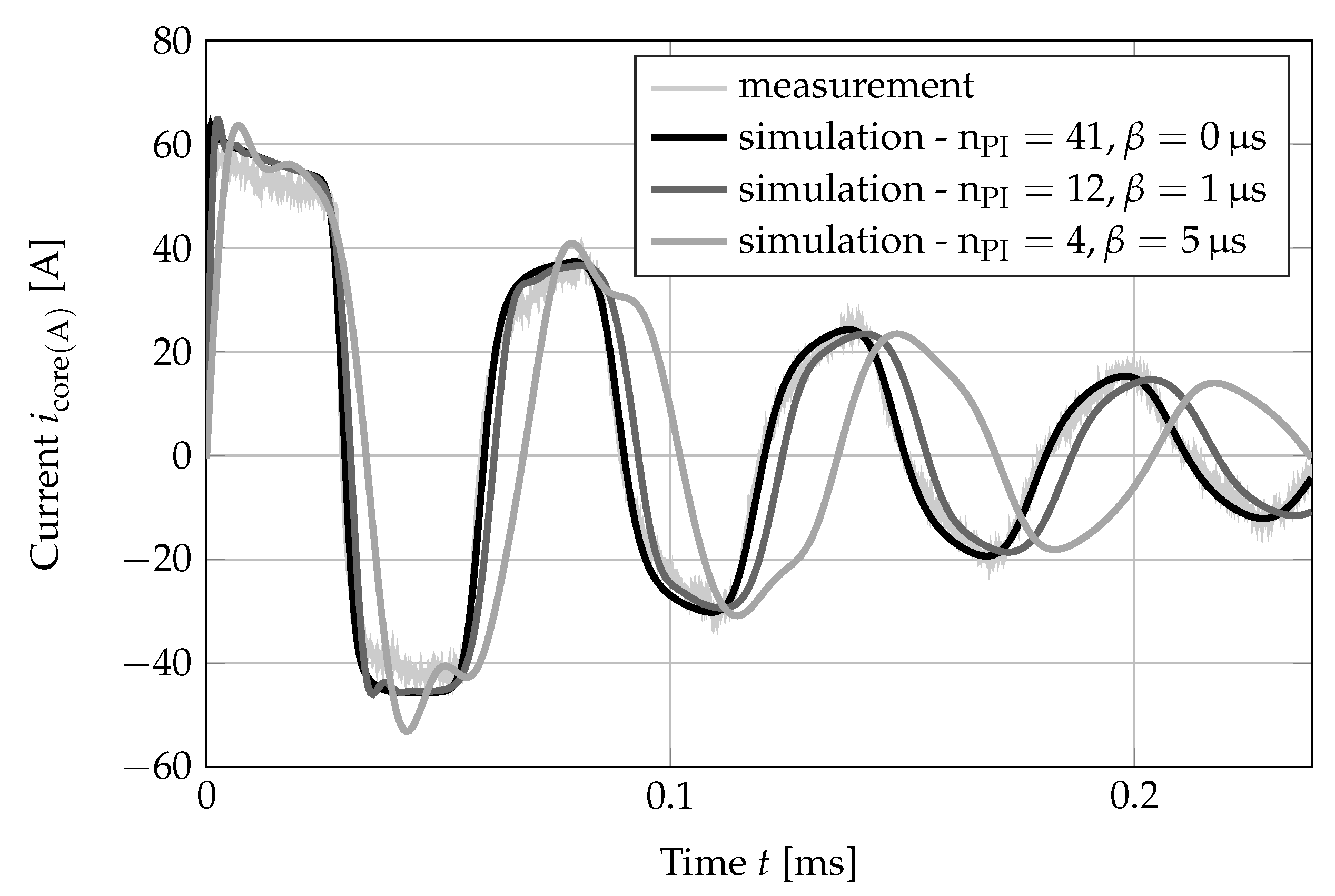
The impact of reducing the number of PI-sections on the simulation results will be illustrated using measured data. The measurements are performed using the same principle already described in Section 4.1. Figure 15 shows the measured current and the simulations with the developed 3P-PI-Model using the previously defined number of PI-sections.
As it can be seen, using the upper limit of PI-sections () in the developed 3P-PI-Model results in a very good match between the measured current and the simulated one. This means that the wave travel time and attenuation are replicated correctly in the developed cable model. The match with the measured current is reduced when specifying an error in the time delay, whereby a worse match will occur by specifying a large error (s).
Reducing the number of PI-sections by specifying an error in the time delay affects the accuracy of the calculations. On the other hand, it results in a significant reduction of the computational effort. In this particular example, the dimension of the equations in the developed 3P-PI-Model are reduced from 6642 by to 1944 by and to 648 by . In addition, the computation time (MATLAB®, typical PC-configuration) is reduced from 5 s by to 2.5 s by and to 2 s by .
5. Conclusions
In this work, detailed investigations of the behavior of a previously developed 3P-PI-Model are introduced. It has been proven that the frequency dependence of cable parameters, the length distribution of PI-sections and the number of PI-sections impact the frequency and the amplitude of the main resonance of PI-sections.
In addition, the number of PI-sections has a big impact on the computational effort in the developed 3P-PI-Model. Using a large number of PI-sections increases the accuracy of the simulation results. On the other hand, the large number of PI-sections leads to a high computational effort.
Two algorithms to optimize the number of PI-sections are developed. In the first algorithm, an upper limit of the number of PI-sections is defined in order to limit the computational effort in the developed 3P-PI-Model.
In the second algorithm, the computational effort of the calculations in the developed 3P-PI-Model is reduced at the expense of the accuracy. To achieve this, the number of PI-sections is defined (starting from the upper limit of PI-sections) after specifying an error in the time delay.
A comparison of the outcomes of the developed 3P-PI-Model using the upper limit of PI-sections with measured data has shown a good match, which validates the approach used in the calculating of the number of PI-sections. In addition, a proper accuracy of the simulation results with a large reduction in the computational effort can be reached by specifying a small error in the time delay.
In this work, the proposed first and second algorithms are used to define the number of PI-sections for simulating of fast transients. However, both algorithms can also be used by different operating states of the power system (e.g., switching operations).
Author Contributions
A.H. realized the investigations on the developed wave propagation model; U.S. calculated the frequency dependent cable parameters; A.G. helped with the measurements.
Funding
The publication costs of this article were funded by the German Research Foundation/DFG and the Technische Universität Chemnitz in the funding programme Open Access Publishing.
Conflicts of Interest
The authors declare no conflict of interest.
References
- Watson, N.; Arrillaga, J. Power Systems Electromagnetic Transients Simulation; The Institution of Engineering and Technology: London, UK, 2007. [Google Scholar]
- Juan, A. Power System Transients: Parameter Determination; CRC Press: Boca Raton, FL, USA, 2009. [Google Scholar]
- Rusek, A.; Ganesan, S.; Aloi, N. A Friendly Approach to Transient Processes in Transmission Lines. In Proceedings of the 2011 ASEE North Central & Illinois-Indiana Section Conference, Mount Pleasant, MI, USA, 1–2 April 2011. [Google Scholar]
- Snelson, J. Propagation of travelling waves on transmission lines—Frequency dependent parameters. IEEE Trans. Power Appar. Syst. 1971, PAS-90, 2561–2567. [Google Scholar] [CrossRef]
- Meyer, W.S.; Dommel, H.W. Numerical Modelling of Frequency-Dependent Transmission-Line Parameters in an Electromagnetic Transients Program. IEEE Trans. Power Appar. Syst. 1974, PAS-93, 1401–1409. [Google Scholar] [CrossRef]
- Dommel, H.W. Digital computer solution of electromagnetic transients in single- and multiphase networks. IEEE Trans. Power Appar. Syst. 1969, PAS-88, 388–399. [Google Scholar] [CrossRef]
- Marti, J. Accurate modelling of frequency-dependent lines in electromagnetic transient simulations. IEEE Trans. Power Appar. Syst. 1982, PAS-101, 147–155. [Google Scholar] [CrossRef]
- Huang, W.; Semlyen, A. Computation of Electro-Magnetic Transients on Three-Phase Transmission Line with Corona and Frequency Dependent Parameters. In Proceedings of the IPST 95, International Conference on Power System Trasients, Lisbon, Spain, 3–7 September 1995; pp. 17–22. [Google Scholar]
- Noda, T.; Nagaoka, N.; Ametani, A. Phase Domain Modeling of Frequency-Dependent transmission Lines by Means of an ARMA Model. IEEE Trans. Power Deliv. 1996, 11, 401–411. [Google Scholar] [CrossRef]
- Noda, T. Application of Frequency-Partitioning Fitting to the Phase-Domain Frequency-Dependent Modeling of Overhead Transmission Lines. IEEE Trans. Power Deliv. 2015, 30, 174–183. [Google Scholar] [CrossRef]
- Hoshmeh, A.; Schmidt, U. A Full Frequency-Dependent Cable Model for the Calculation of Fast Transients. Energies 2017, 10, 1158. [Google Scholar] [CrossRef]
- Schmidt, U.; Shirvani, A.; Probst, R. An improved algorithm for determination of cable parameters based on frequency-dependent conductor segmentation. In Proceedings of the IEEE PES Transmission and Distribution Conference, Montevideo, Uruguay, 3–5 September 2012; pp. 241–246. [Google Scholar]
- Schmidt, U. Frequenzabhängige Parameter von Kabeln zur Berechnung von Ausgleichsvorgängen im. Zeitbereich. Dissertation, Technische Universität Chemnitz, Ilmenau, Germany, 2013. [Google Scholar]
- Gustavsen, B.; Semlyen, A. Rational approximation of frequency domain responses by Vector Fitting. IEEE Trans. Power Deliv. 1999, 14, 1052–1061. [Google Scholar] [CrossRef]
- Gustavsen, B. Improving the pole relocating properties of vector fitting. IEEE Trans. Power Deliv. 2006, 21, 1587–1592. [Google Scholar] [CrossRef]
- Marti, L. Simulation of Electromagnetic Transients in Underground Cables with Frequency-Dependent Modal Transformation Matrices. Ph.D. Thesis, The University of British Columbia, Vancouver, BC, Canada, 1986. [Google Scholar]
- Chrysochos, A.I.; Papadopoulos, T.A.; Papagiannis, G.K. Robust Calculation of Frequency-Dependent Transmission-Line Transformation Matrices Using the Levenberg Marquardt Method. IEEE Trans. Power Deliv. 2014, 29, 1621–1629. [Google Scholar] [CrossRef]
- Gustavsen, B.; Semlyen, A. Combined phase and modal domain calculation of transmission line transients based on vector fitting. IEEE Trans. Power Deliv. 1998, 13, 596–604. [Google Scholar] [CrossRef]
- Marti, J. The Problem of Frequency Dependence in Transmission Line Modelling. Ph.D. Thesis, The University of British Columbia, Vancouver, BC, Canada, 1981. [Google Scholar]
- Marti, L. Simulation of transients in underground cables with frequency dependent modal transformation matrix. IEEE Trans. Power Appar. Syst. 1988, 3, 1099–1110. [Google Scholar] [CrossRef]
- Hoshmeh, A.; Malekian, K.; Schufft, W.; Schmidt, U. A single-phase cable model based on lumped-parameters for transient calculations in the time domain. In Proceedings of the 15th International Conference on Environment and Electrical Engineering (EEEIC 2015), Rome, Italy, 10–13 June 2015; pp. 731–736. [Google Scholar]
- Scott-Meyer, W. EMTP—Rule Book: Manual, Bonneviller Power Administration; European EMTP–ATP Users Group: Offenbach, Germany, 1982. [Google Scholar]
- Hadid, S. Verlustfaktor-Messung an PE/VPE-isolierten Mittelspannungskabeln bei veränderlicher Frequenz; Interner forschungsbericht, Technische Universität Chemnitz: Chemnitz, Germany, 2011. [Google Scholar]
- Hadid, S.; Schmidt, U.; Schufft, W.; Rätzke, S. Frequenzabhängigkeit des Verlustfaktors tan δ an VPE-isolierten Kabeln. ETG-Fachtagung, Diagnostik elektrischer Betriebsmittel 2012. [Google Scholar]
- Dommel, H.W. Electromagnetic Transients Program Manual (EMTP Theory Book); Bonneville Power Administration: Portland, OR, USA, 1986. [Google Scholar]
- Ametani, A. A general formulation of impedance and admittance of cables. IEEE Trans. Power Appar. Syst. 1980, PAS-99, 902–909. [Google Scholar] [CrossRef]
- Dommel, H.W. Computation of cable impedances based of subdivision of conductors. IEEE Trans. Power Deliv. 1987, PWRD-2, 21–27. [Google Scholar]
- Lucas, R.; Taluktar, S. Advances in finite elemente techniques for calculation cable resistances and inductances. EEE Trans. Power Appar. Syst. 1978, PAS-9711, 875–883. [Google Scholar] [CrossRef]
- Hedman, D.E. Propagation on overhead Transmission Lines: I. Theory of Modal Analysis; II. Earth-Conduction Effects and Ptactical Results. IEEE Trans. 1965, 110, 200–211. [Google Scholar]
- Semlyen, A.; Dabuleanu, A. Fast and Accurate Switching Transient Calculations on Transmission Lines With Ground Return Using Recursive Convolutions. IEEE Trans. Power Appar. Syst. 1975, 94, 561–571. [Google Scholar] [CrossRef]
- Garcia, N.; Acha, E. Transmission Line Model with Frequency Dependency and Propagation Effects: A Model Order Reduction and State-Space Approach. In Proceedings of the 2008 IEEE Power and Energy Society General Meeting—Conversion and Delivery of Electrical Energy in the 21st Century, Pittsburgh, PA, USA, 20–24 July 2008; pp. 1–7. [Google Scholar]
Figure 1.
Representation of the frequency dependence of the cable longitudinal impedance.
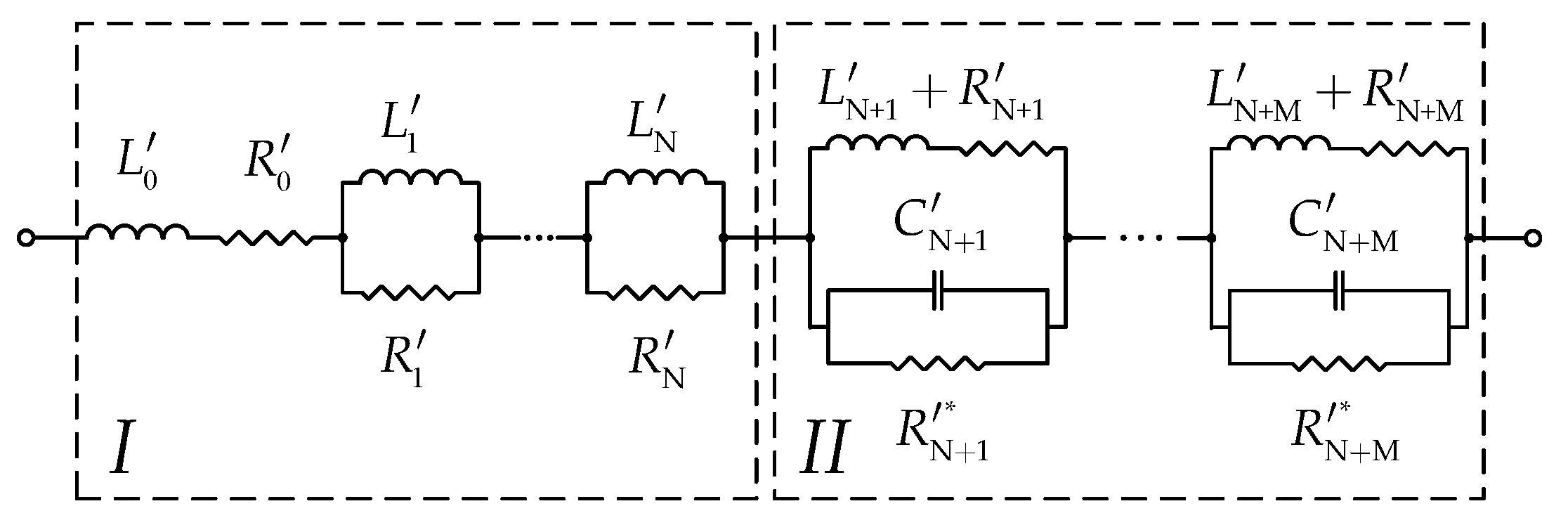
Figure 2.
PI-section with the frequency dependence.
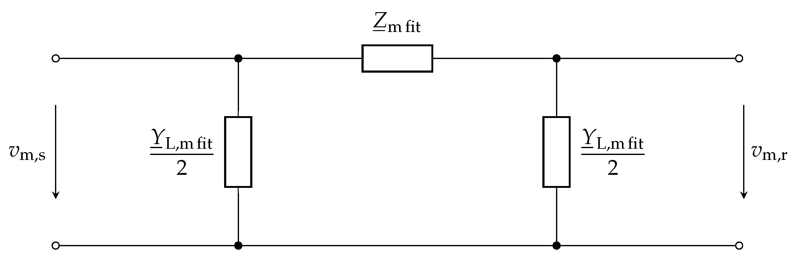
Figure 3.
Principle of the 3phase cable model.
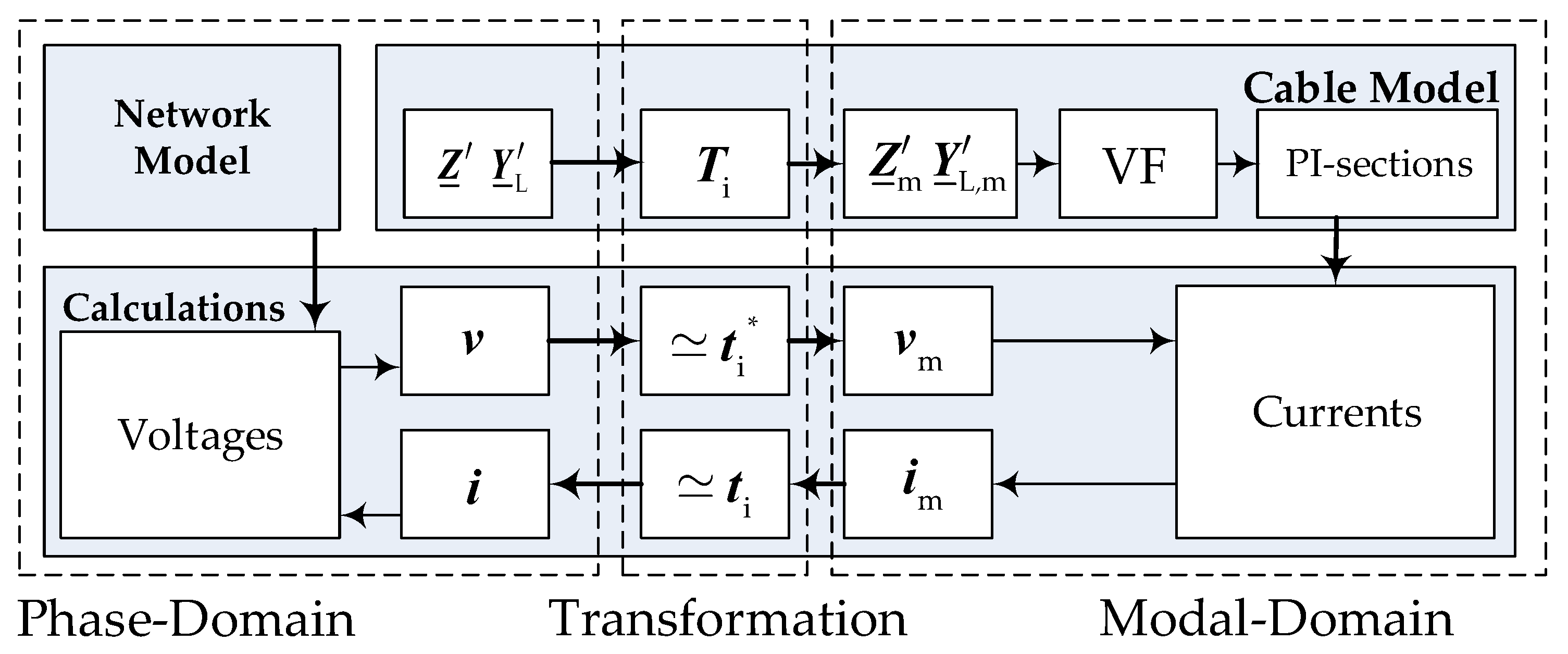
Figure 4.
Traditional PI-section without the frequency dependence.

Figure 5.
Amplitude of cable impedance at sending end with and without considering the frequency dependence (traditional and developed 3P-PI-Model), , km.
Figure 5.
Amplitude of cable impedance at sending end with and without considering the frequency dependence (traditional and developed 3P-PI-Model), , km.

Figure 6.
Length distribution profiles of PI-sections.
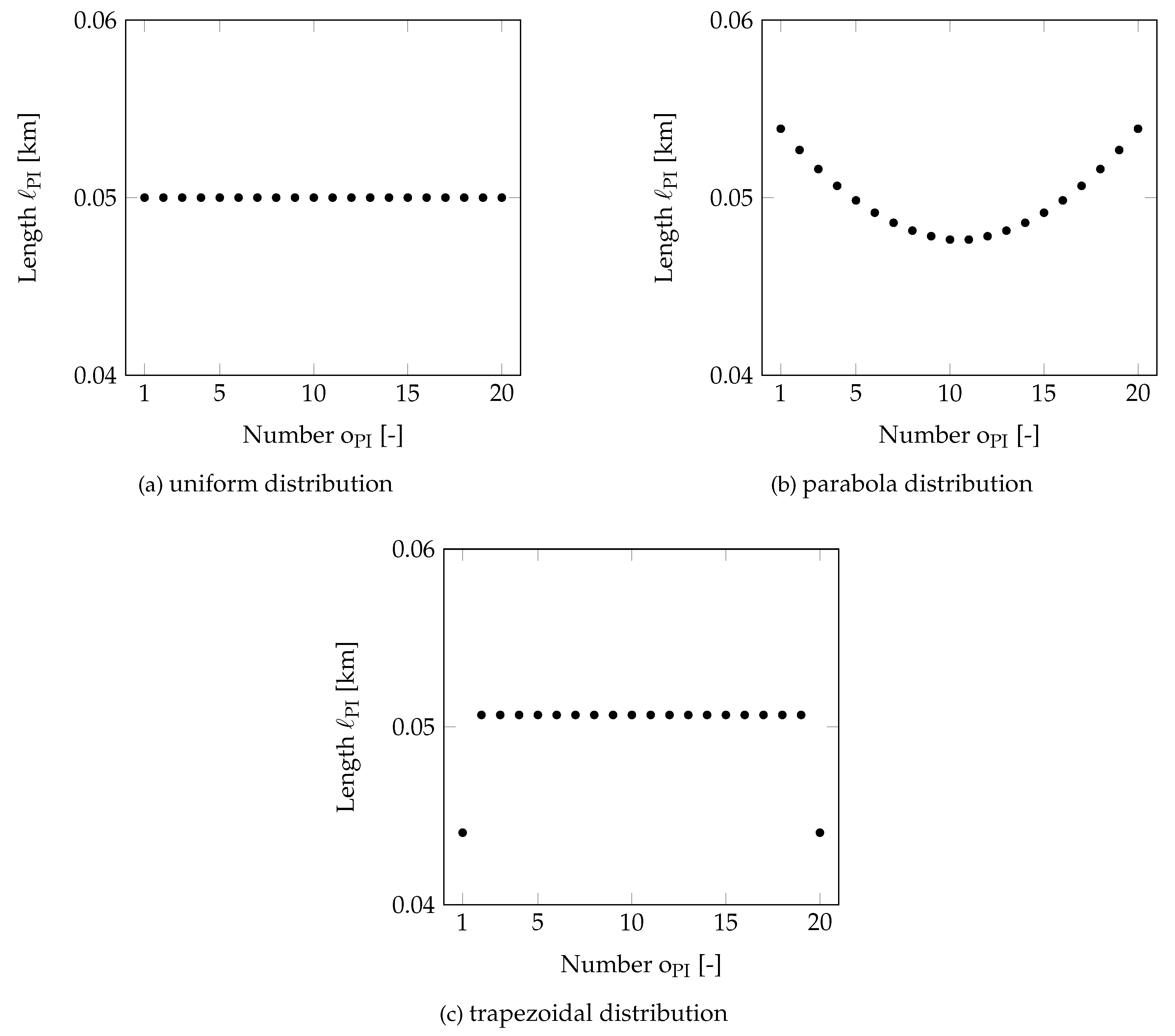
Figure 7.
Amplitude of cable impedance at sending end for different length distribution profiles of PI-sections, , km.
Figure 7.
Amplitude of cable impedance at sending end for different length distribution profiles of PI-sections, , km.
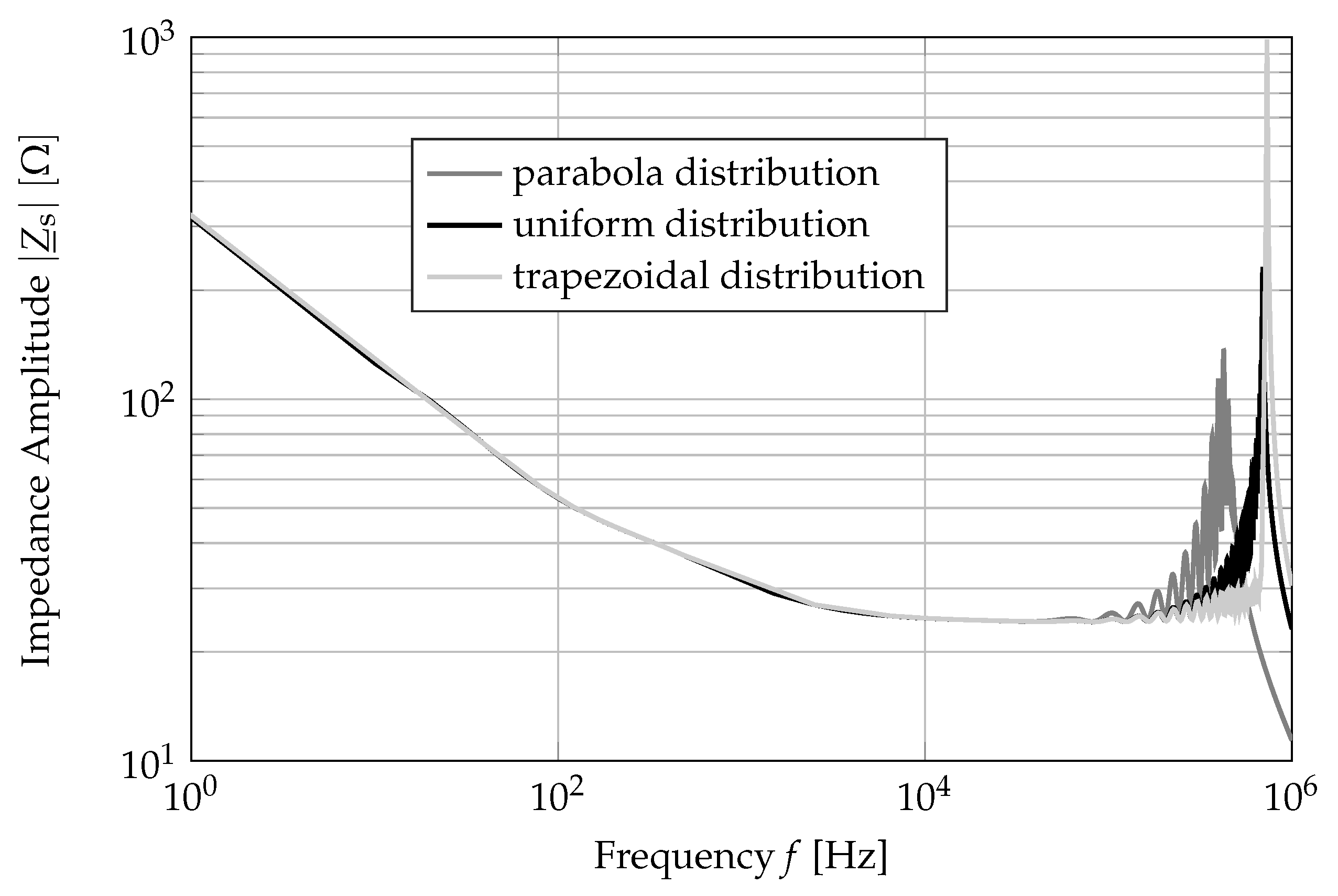
Figure 8.
Impedance amplitude for the distributed-parameters model and developed 3P-PI-Model with two different numbers of PI-sections, km.
Figure 8.
Impedance amplitude for the distributed-parameters model and developed 3P-PI-Model with two different numbers of PI-sections, km.
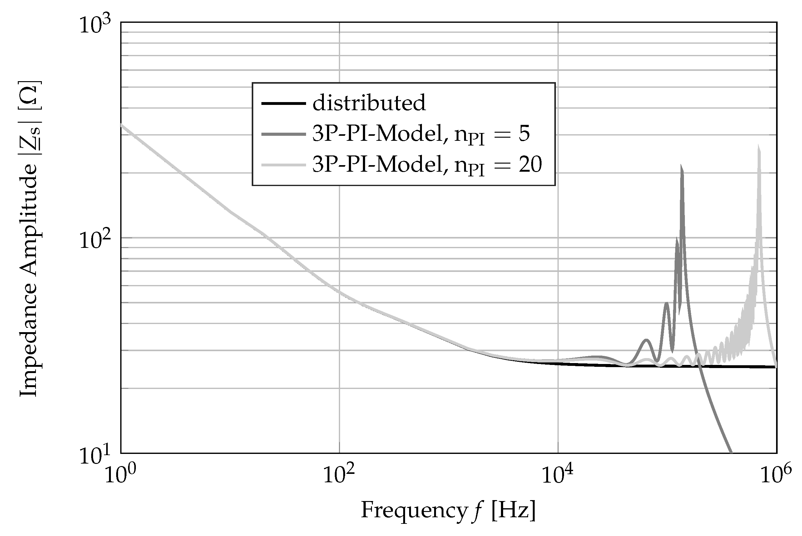
Figure 9.
Configuration for the DC-Test.
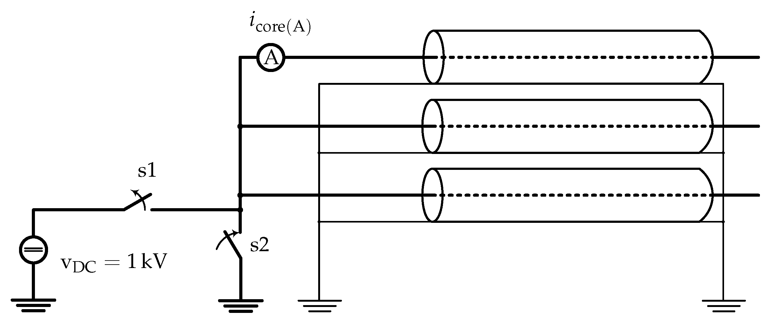
Figure 10.
Simulations of the discharge current with different number of PI-sections.
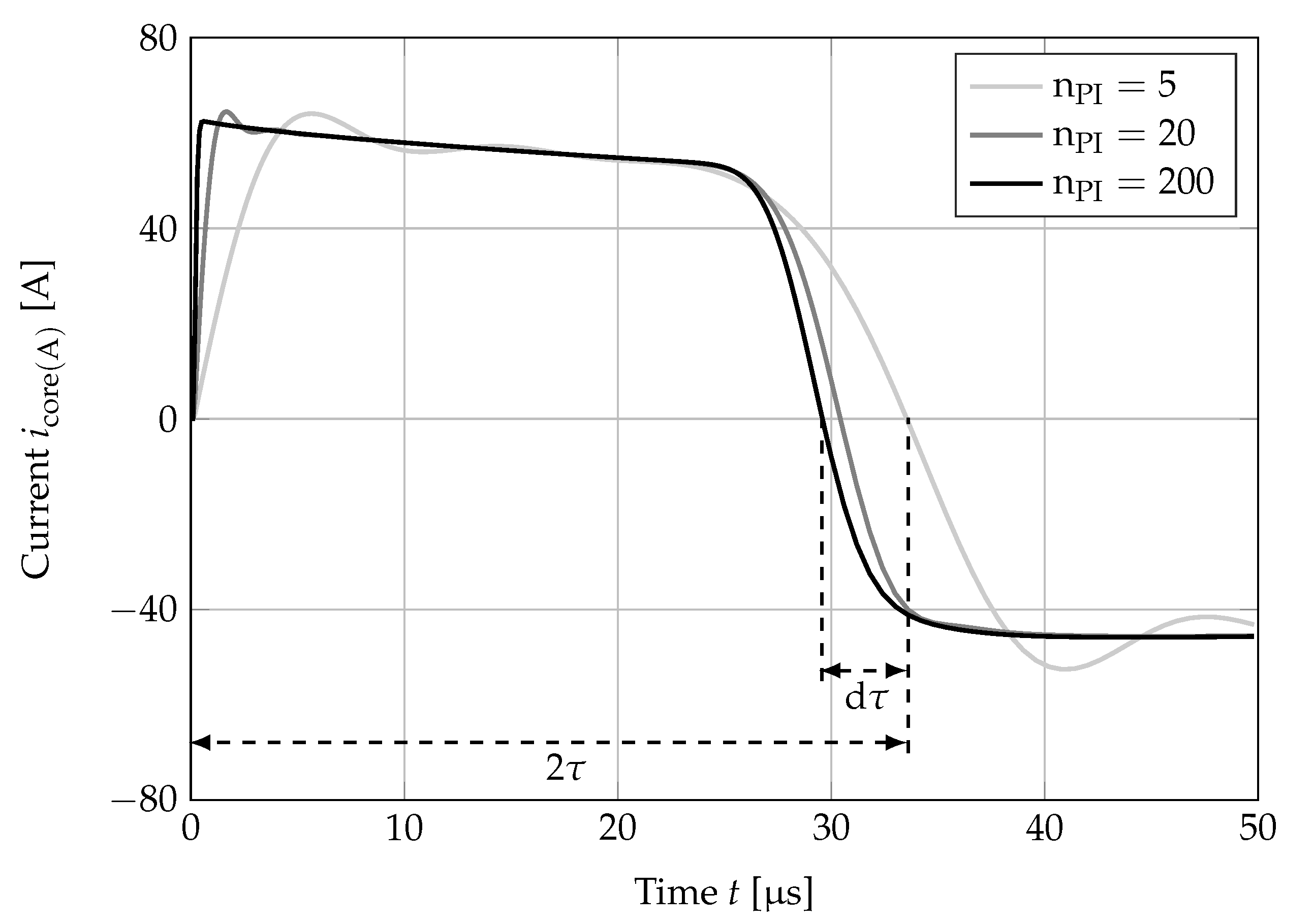
Figure 11.
Optimization the number of PI-sections—first algorithm.
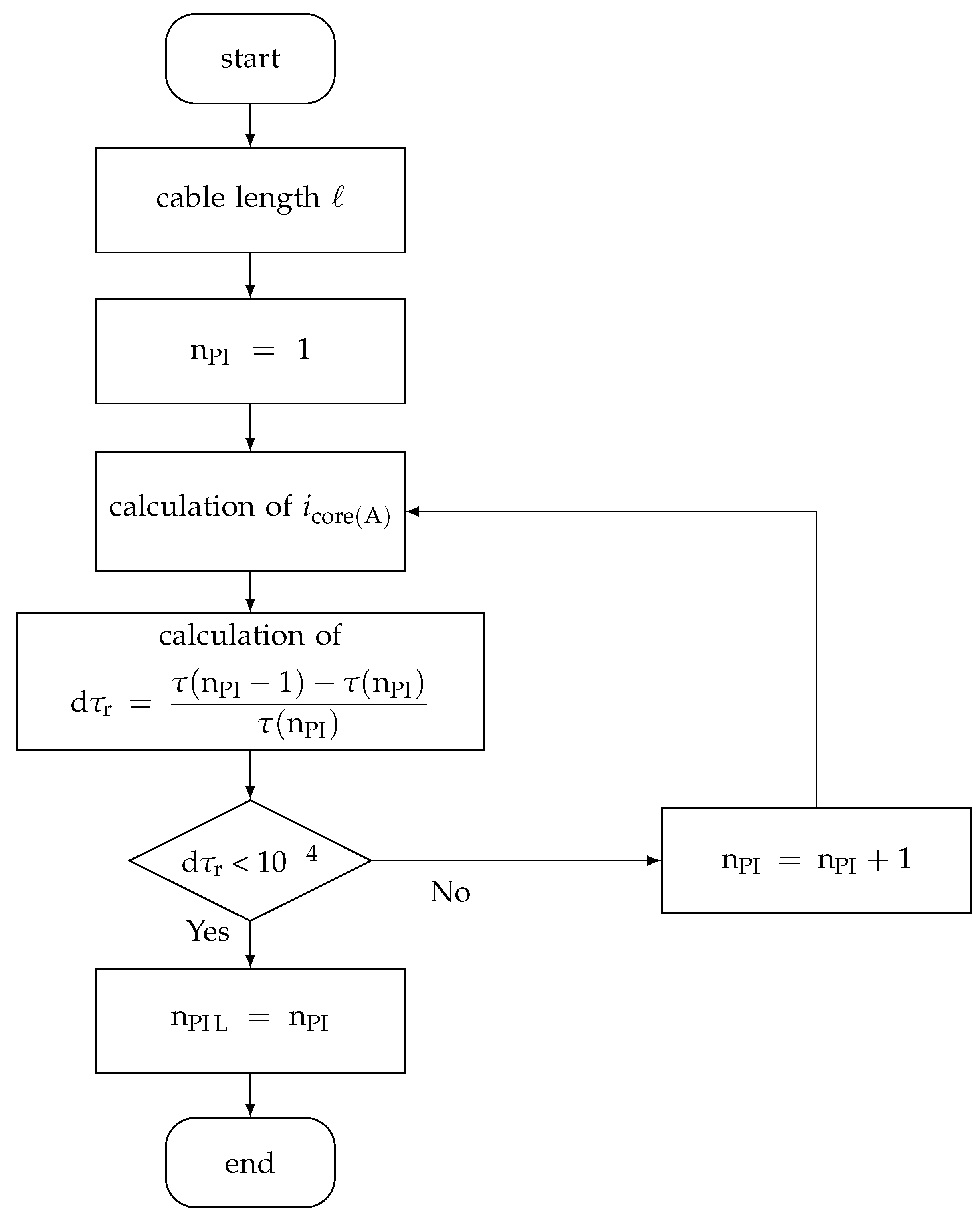
Figure 12.
The upper limit of PI-sections for different cable lengths.
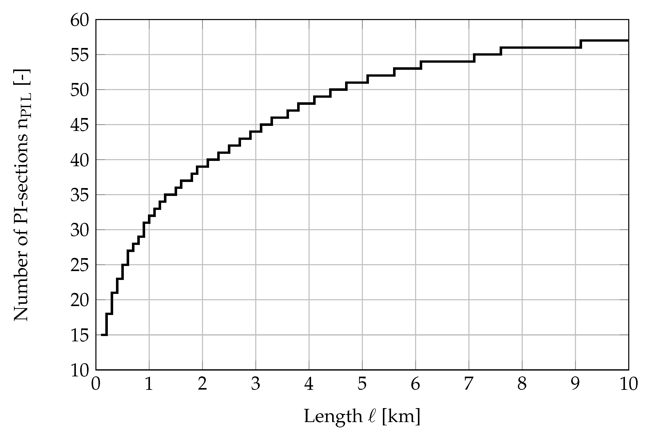
Figure 13.
Optimization the number of PI-sections—second algorithm.

Figure 14.
Number of PI-sections for different specified error in the time delay.
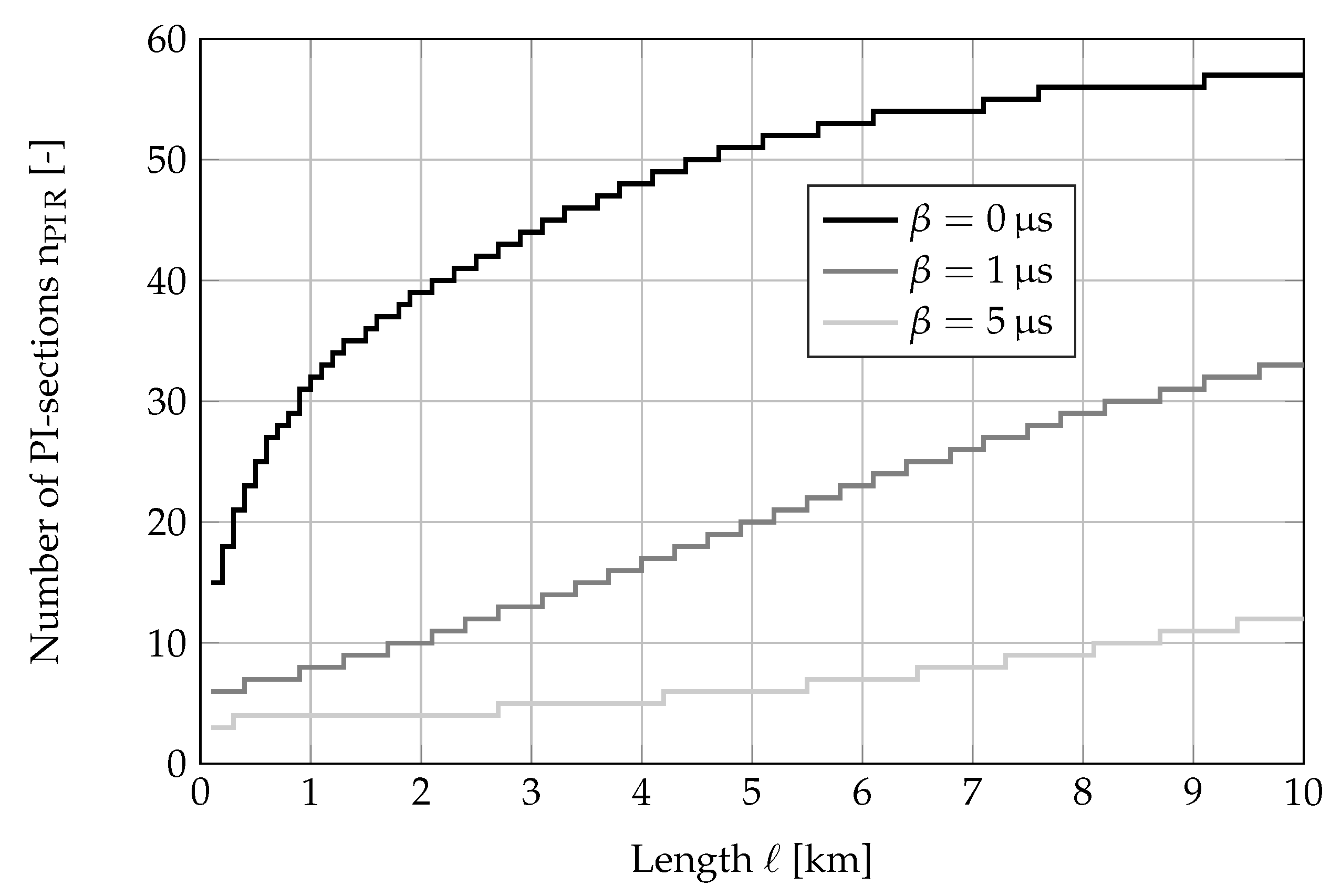
Figure 15.
Comparison of simulated currents by different number of PI-sections with measurements.


Table 1.
Parameters of 10 kV cable, NA2XS(FL)2Y.
| Name | Unit | Value |
|---|---|---|
| Outer radius of the core | ||
| Inner radius of the sheath | ||
| Outer radius of the sheath | ||
| Outer insulation radius | ||
| Core resistivity | ||
| Shield resistivity | ||
| Inner insulation | ||
| Outer insulation | ||
| Inner insulation relative permittivity | ||
| Outer insulation relative permittivity | ||
| Relative permeability | ||
| Earth resistivity | 150 | |
| Type of installation | Trefoil | |
| Laying depth (system center) | ||
| Length | ℓ |
© 2018 by the authors. Licensee MDPI, Basel, Switzerland. This article is an open access article distributed under the terms and conditions of the Creative Commons Attribution (CC BY) license (http://creativecommons.org/licenses/by/4.0/).
Share and Cite
MDPI and ACS Style
Hoshmeh, A.; Schmidt, U.; Gürlek, A. Investigations on the Developed Full Frequency- Dependent Cable Model for Calculations of Fast Transients. Energies 2018, 11, 2390. https://doi.org/10.3390/en11092390
AMA Style
Hoshmeh A, Schmidt U, Gürlek A. Investigations on the Developed Full Frequency- Dependent Cable Model for Calculations of Fast Transients. Energies. 2018; 11(9):2390. https://doi.org/10.3390/en11092390
Chicago/Turabian StyleHoshmeh, Abdullah, Uwe Schmidt, and Akif Gürlek. 2018. "Investigations on the Developed Full Frequency- Dependent Cable Model for Calculations of Fast Transients" Energies 11, no. 9: 2390. https://doi.org/10.3390/en11092390
Note that from the first issue of 2016, this journal uses article numbers instead of page numbers. See further details here.