1. Introduction
Underground cables are an important part of electrical power systems in the HV, the EHV and the UHV level. Their application and the impact has increased with the growth of wind and solar energy to the total electricity generation [
1,
2]. The knowledge about the behavior in cases of transients is required for the correct design of cable lines and the overvoltage protection. The major difficulty for the modeling of cables is the complexity of the geometrical configuration and the electromagnetic coupling between phase conductors, cable shield and the earth. For this case, applicable models are required for the calculation of the electrical stresses. Effective models exist for load flow calculations and for calculations in the frequency domain. Older models were derived from approaches for overhead line calculations [
3,
4,
5,
6,
7,
8,
9,
10]. The results of these models have problems with result accuracy and the robustness. The incorrect modeling of geometrical condition and the incomplete interpretation of electromagnetic coupling are the reasons for the problems. To achieve a proper accuracy, a model with exact frequency-dependent cable parameters and with a good reproduction of wave propagation behavior is required.
In [
11] a new full frequency-dependent three-phase PI-section cable model (3P-PI-Model) is introduced and validated. The frequency-dependent impedances in the model are determined with an improved sub-conductor method considering the skin and the proximity effect in the core, the shield and the earth [
12,
13]. The wave propagation in the model is based on PI-sections. The frequency dependence of the cable parameters is reproduced by means of vector fitting algorithm [
14,
15] and implemented through an RLC-network in a defined number of PI-sections. To decouple the three-phase cable system, a modal transformation is used [
16,
17,
18].
For the implementation in calculation software, it is important to understand the behavior and the impact of the model parameter to the results. The significant problems of using PI-sections are their main resonance and the computational effort, which results from working with a large number of PI-sections. These problems can be influenced in the developed 3P-PI-Model through different parameters. The most important parameters, which have a direct impact, are the frequency dependence of cable parameters, length distribution of PI-sections and the number of PI-sections. To reduce the computational effort in the new model, two algorithms have been introduced for optimizing the number of PI-sections.
2. Wave Propagation Cable Model
The wave propagation in a multi-conductor cable or transmission line can be represented in the frequency domain with second-order differential Equations [
19]:
The longitudinal impedances
and the shunt admittance
in the phase domain are calculated using the developed algorithms in [
12,
13]. The index “L” stands for lateral. In order to solve the differential Equations (
1) and (
2), a modal transformation technique has been proposed in [
19]. As a result, the coupling between the cable conductors disappears and the cable system can be considered as decoupled single conductors. In the modal domain, Equations (
1) and (
2) can be rewritten as:
where
is a diagonal matrix which represents the eigenvalues matrix of
and
. For the transformation into modal domain the modal transformation matrices
and
are used. The relation between the matrices is given in [
20]:
Therefore, it is sufficient to calculate only one of them. In this paper, the results for
will be calculated as in [
17]. In order to perform the calculation in the modal domain, the quantities
,
,
and
have to be transformed into this domain. From Equations (
3) and (
4), it can be derived:
With simple matrix perturbation, the above equations are then rewritten as:
By rearranging the terms and by using the Equation (
5) in (
8) and (
9), the longitudinal impedance and the shunt admittance in the modal domain can be defined as:
Both matrices in Equations (
10) and (
11) are diagonal. The frequency dependence of the elements of
cannot be neglected (as assumed for the elements of
). This is related to the frequency dependent elements of
. The elements of
are also strong frequency dependent. In order to take the frequency dependency of
and
into account, their diagonal elements will be approximated by mathematical functions using the vector fitting algorithm (VF) [
14,
15]. For example, the first diagonal element in
can be approximated using VF as:
The accuracy of
depends on the number of the real terms N and the number of the complex terms M.
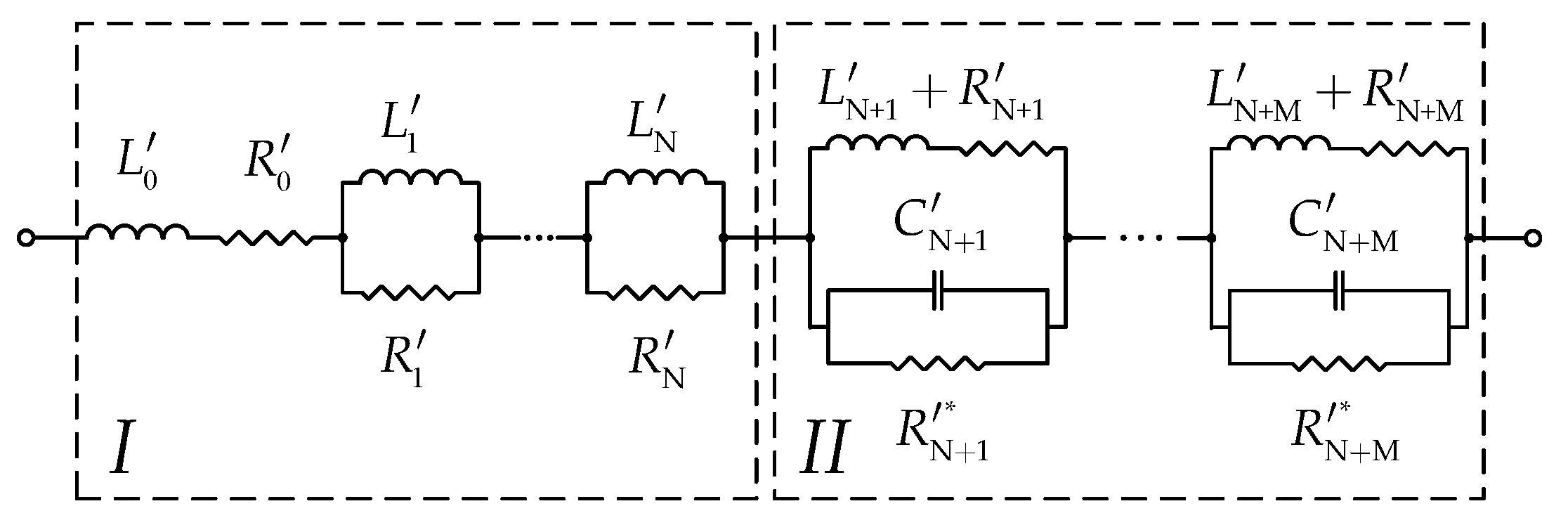
can be reproduced with an electrical network. In [
21], a RL-network has been used. Using such a network allows to employ only the real poles and residues in the approximation (the complex terms are discarded). Although the fitting is achieved with a low order of approximation, the accuracy is affected. In this paper, an RLC-network shown in
Figure 1 is introduced to regard all the poles and residues in the approximation including the complex terms.
As can be seen, the network has been divided into two sections. The elements of the section
I can be evaluated in a similar way as in [
21]. The elements of section
II are obtained as follows:
The first diagonal element of
is similarly approximated. Furthermore,
and
are assumed to be zeros in
. After calculating
and
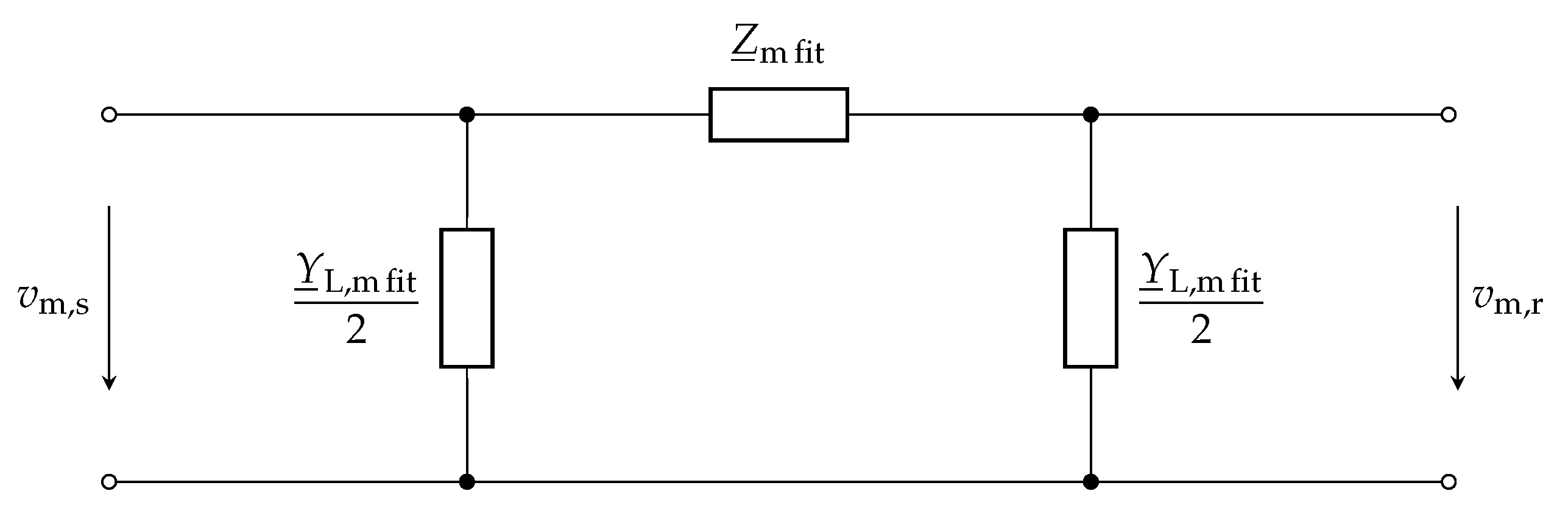
, they will be combined to form a developed PI-section.
Figure 2 shows a representation for the developed PI-section after regarding the cable length, where
and
are the voltages in the modal domain at sending and receiving end respectively. One single conductor in the developed cable model can then be represented by cascading a number of PI-sections. Basically, the number of PI-sections depends on the cable length.
For the remaining diagonal elements of
and
, the same procedure is used to form the other conductors in the developed cable model. From the Equations (
3)–(
5), the voltages and the currents are transformed into the modal domain as follows:
The Equations (
14) and (
15) are still in the frequency domain. However, since the simulations in the power system are necessary in the time domain, these equations have to be transformed into this domain. For the voltages in Equation (
14), the convolution integral is applied as:
Evaluation of this integral point by point is time consuming. By approximating the elements of
using rational functions, an efficient recursive convolution method is used [
7] and the above integral can be rewritten as a sum of exponentials:
where
b and
l are the approximations parameters of the rational functions. The wave travel time
for the impulse from one end of the cable to the other one is related to the imaginary term of the propagation function
:
The voltage vector
is calculated recursively from
as:
In this relation,
,
and
are constants that mainly depend on
b,
l and
[
19]. The same procedure is used to transform the currents in Equation (
15) into the time domain. In order to execute the time domain simulations, the differential equations for single conductors in the developed cable model have to be formulated. As shown in [
21], the differential equations can be represented using state space techniques. A numerical Backward Euler rule of integration can then be applied to find the solution for the related state space equations [
22]. To solve the cable equations with the rest of the network, which is always defined in phase quantities, the calculated voltages and currents in the modal domain must be transformed back to phase quantities.
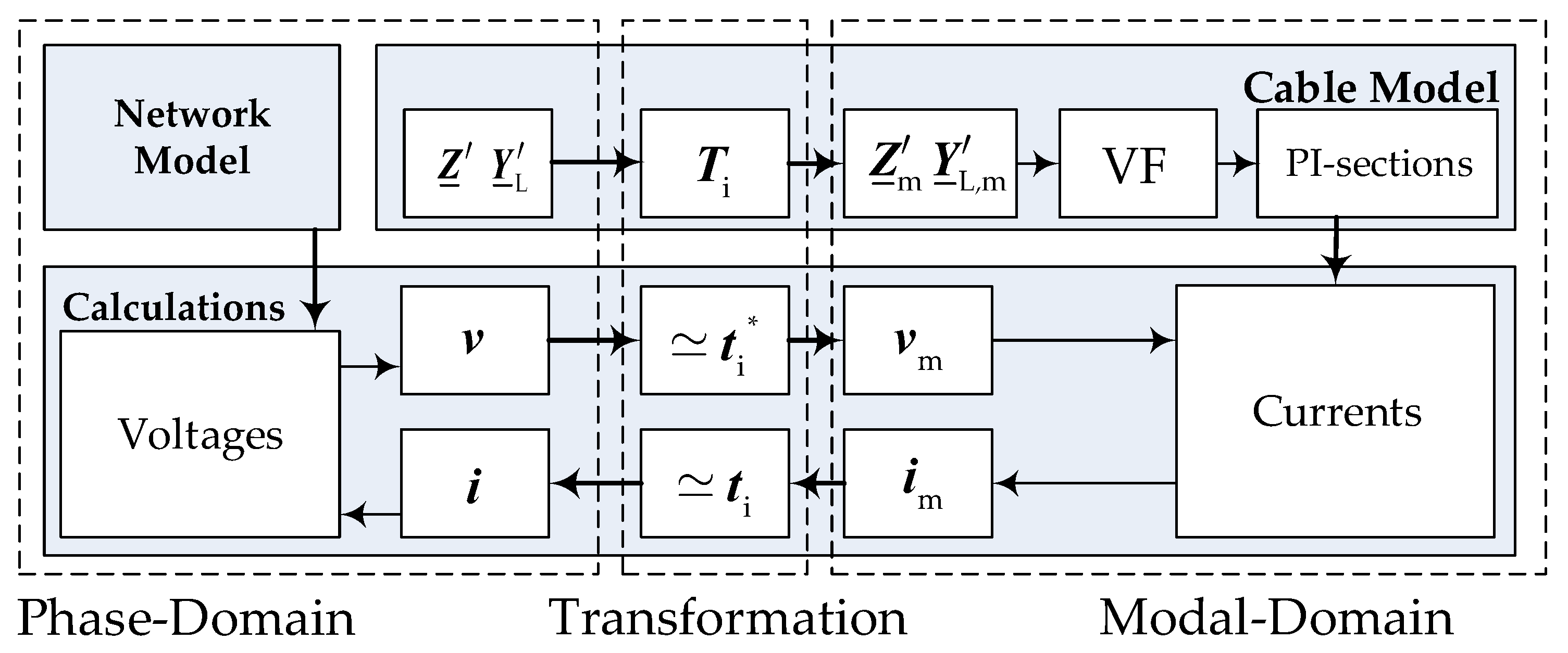
Figure 3 shows an overview for the realization of the 3P-PI-Model.
Starting from defining and , the cable model part is executed only once to provide the PI-sections for the calculation part. In this part, the computation is evaluated every . For the first one, the vector of the voltages is calculated using the network model and the vector of the currents . By applying the recursive convolution between and the approximation of (), the vector of the voltages is calculated. Using the PI-sections and , the state space equations are formulated and solved by means of numerical Backward Euler rule of integration to yield the current vector . The recursive convolution between and the approximation of () provides the vector of currents for the next .
4. Analysis in the Time Domain
For modeling of cables with PI-sections, a minimum number of these sections has to be used. The number of PI-section depends mainly on the cable length and the simulated event. The longer the cable is, the more PI-sections are needed. In addition, more PI-sections are needed to simulate transient events (e.g., lightning strikes or switching operations) compared to steady state operations (e.g., during normal operation or failure).
4.1. Optimization of the Number of PI-Sections—First Algorithm
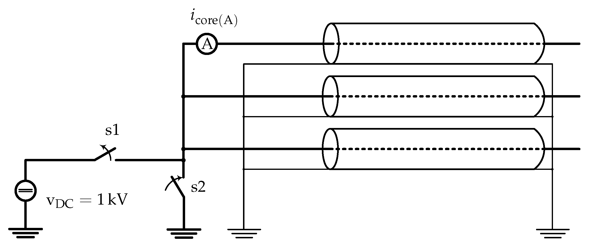
For optimizing the number of PI-sections in the developed 3P-PI-Model, a DC-Test on a three-phase cable with a length of
in trefoil formation has been used. The test is performed by charging the cable conductors up to 1 kV. After that, the charged conductors are connected to earth through the circuit breaker (s2) and the discharge current
at the sending end is simulated. The test configuration is shown in
Figure 9. The cable parameters are given in
Table 1.
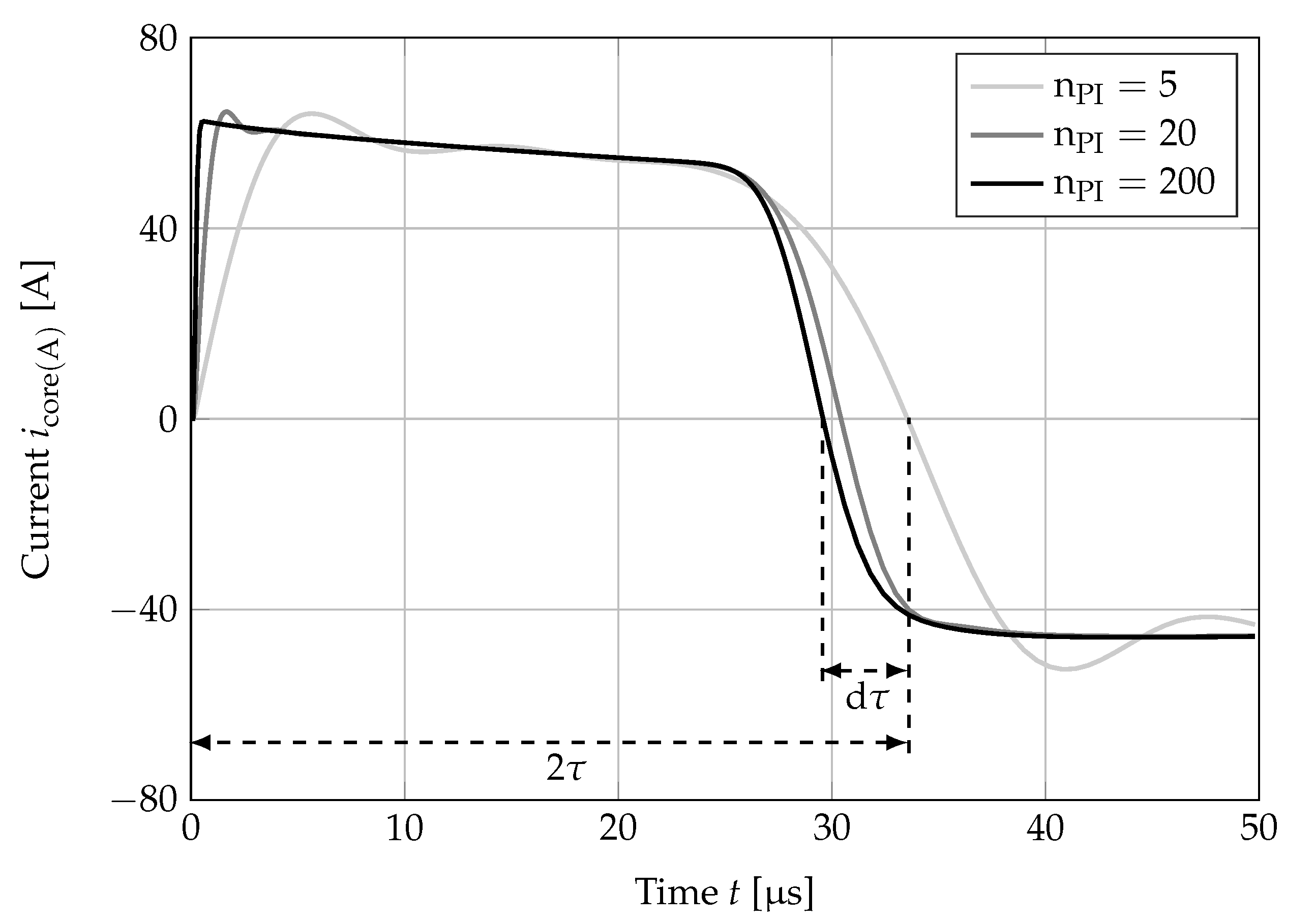
Figure 10 shows the discharge current
with different number of PI-sections.
As it can be seen, the slope of the current increases and the time delay of the current
decreases. This is mainly due to the better replication of the higher frequencies in the current by increasing the number of PI-sections. However, the change in time delay
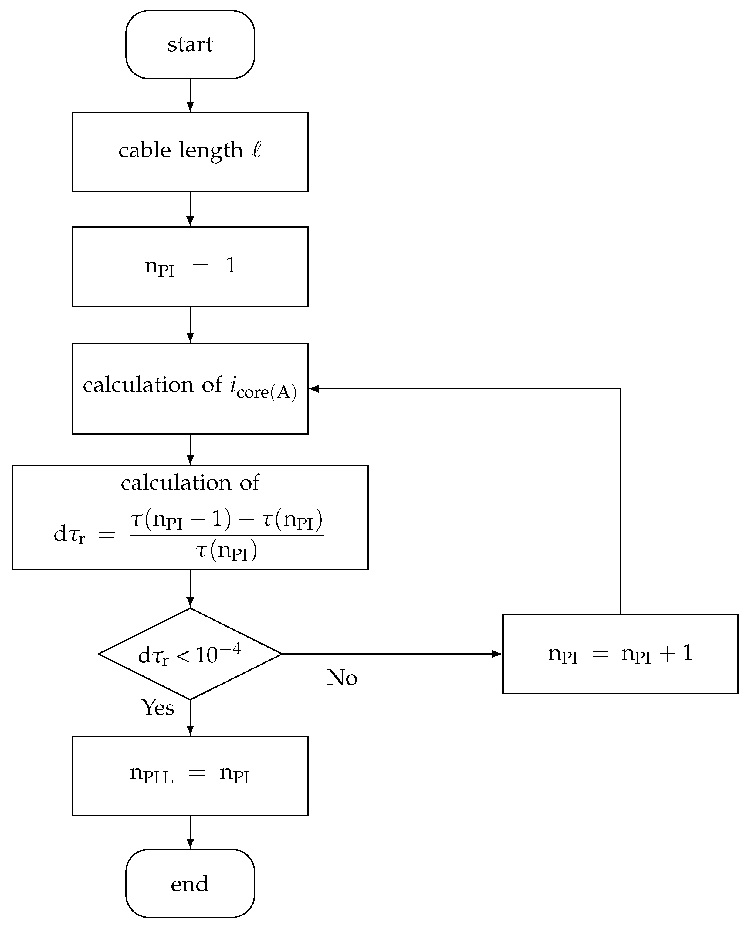
becomes smaller as the number of PI-sections increases. Above a certain number of PI-sections, this change can be neglected. Therefore, it is useful to set an upper limit on the number of PI-sections to optimize the computational effort. The upper limit of the number of PI-sections is determined using the algorithm shown in
Figure 11.
For a given cable length ℓ, the number of PI-sections increases until the relative change in the time delay is less than a defined limit. The limit is initially set to . If the time delay is lower than this limit, then the loop is interrupted and the reached number of PI-sections is stored as the upper limit .
In this context, it should be noted that the overshoot of the current in
Figure 10 (e.g., in the range
s) is minimized and thus the amplitude of the current is also optimized by optimizing the time delay of the current. The reason is the dependence of the amplitude of the current on the characteristic impedance of the cable. This characteristic impedance is mainly calculated from the inductance and the capacitance of the cable, which in turn are included in the calculation of the time delay (see Equation (
23)).
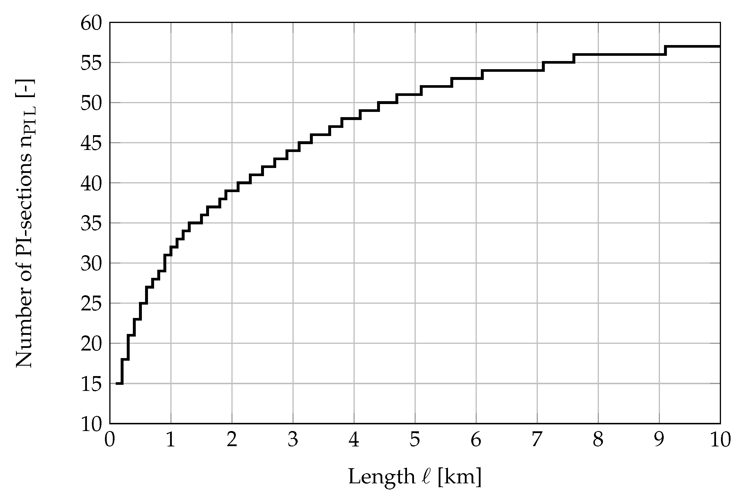
Figure 12 shows the upper limit of the number of PI-sections depending on the cable length in the range
km.
For accurate simulation results, the number of PI-sections must be increased until the frequency of their main resonance is greater than the highest frequency of the event to be simulated. By increasing the cable length, the frequency of the main resonance of PI-sections will decrease [
25]. In order to get the same accuracy of the calculations, the number of PI-sections has to be increased as it can be seen in
Figure 12. For example, to simulate of transients by a cable length of 2.5 km the number of PI-sections is 45 and by a cable length of 10 km this number will increase to 52.
The proposed algorithm shown in
Figure 11 defined the number of PI-sections in order to reach very good accuracy in the developed 3P-PI-Model, which results in using a large number of PI-sections. However, in many cases of simulation of transients a proper accuracy can be accepted. Therefore, the large number of PI-sections can be reduced and thus so can the computational effort.
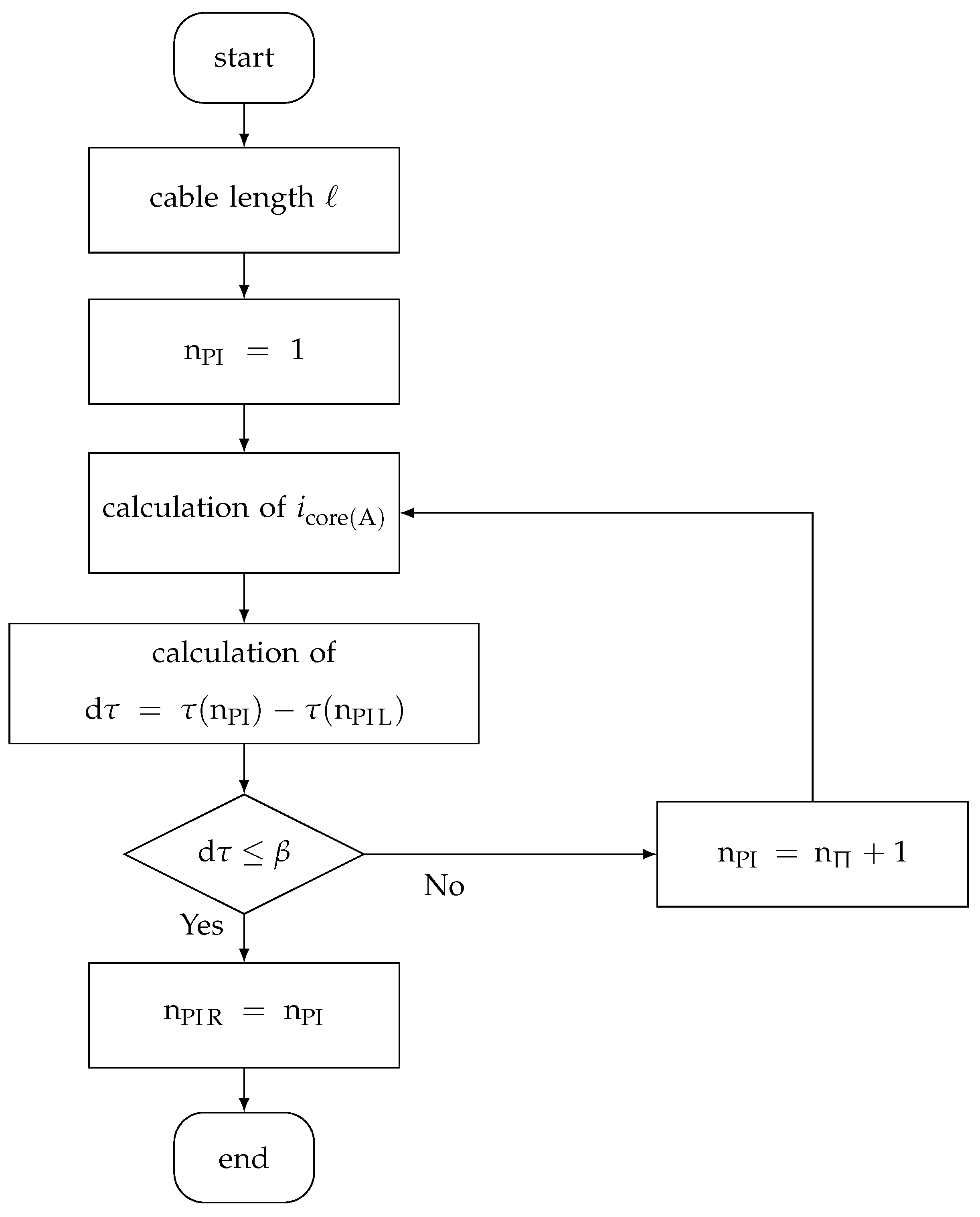
4.2. Optimization of the Number of PI-Sections—Second Algorithm
The main idea of the second algorithm is to reduce the computational effort of the calculations in the developed 3P-PI-Model at the expense of the accuracy.
Figure 13 illustrates the methodology of the second algorithm for the example shown in
Figure 9. In this algorithm, the number of PI-sections is reduced to such an extent that a given error
in the time delay
with respect to a reference value is not exceeded. The number of PI-sections will store under the reduced number
. The reference value of the time delay is defined at upper limit by the number of PI-section
, whereat the error in the time delay
is equal to
s.
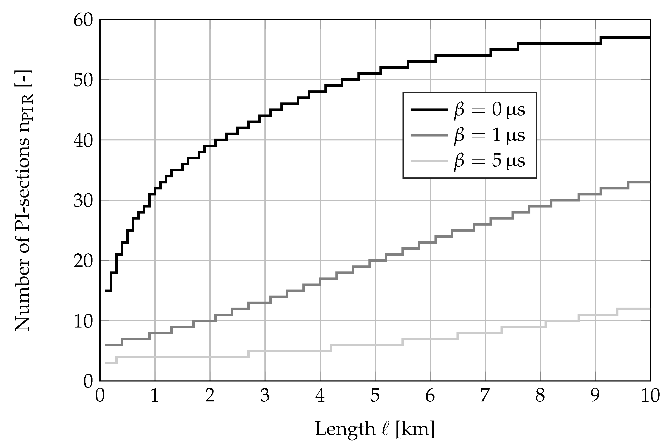
By using the upper limit of the number of PI-sections shown in
Figure 12 in the second algorithm the reduced number of PI-sections can be calculated for different errors in the time delay.
Figure 14 shows the results for two specified errors.
As it can be seen, specifying an error in the time delay leads to a considerable reduction in the number of PI-sections compared to their upper limit. For example, by a cable length of 2.5 km the number of PI-sections decreases from 41 to 12 by s and to 4 by s.
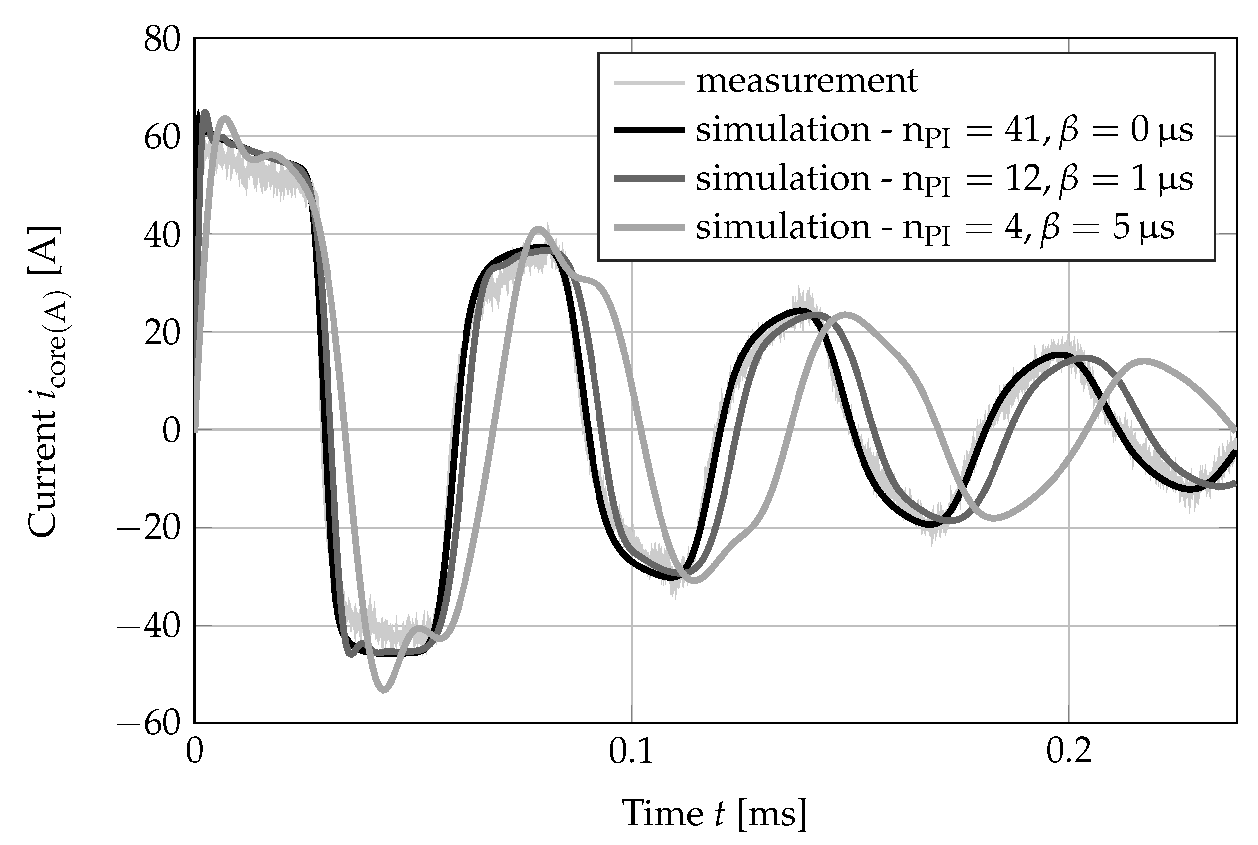
The impact of reducing the number of PI-sections on the simulation results will be illustrated using measured data. The measurements are performed using the same principle already described in
Section 4.1.
Figure 15 shows the measured current and the simulations with the developed 3P-PI-Model using the previously defined number of PI-sections.
As it can be seen, using the upper limit of PI-sections () in the developed 3P-PI-Model results in a very good match between the measured current and the simulated one. This means that the wave travel time and attenuation are replicated correctly in the developed cable model. The match with the measured current is reduced when specifying an error in the time delay, whereby a worse match will occur by specifying a large error (s).
Reducing the number of PI-sections by specifying an error in the time delay affects the accuracy of the calculations. On the other hand, it results in a significant reduction of the computational effort. In this particular example, the dimension of the equations in the developed 3P-PI-Model are reduced from 6642 by to 1944 by and to 648 by . In addition, the computation time (MATLAB®, typical PC-configuration) is reduced from 5 s by to 2.5 s by and to 2 s by .
5. Conclusions
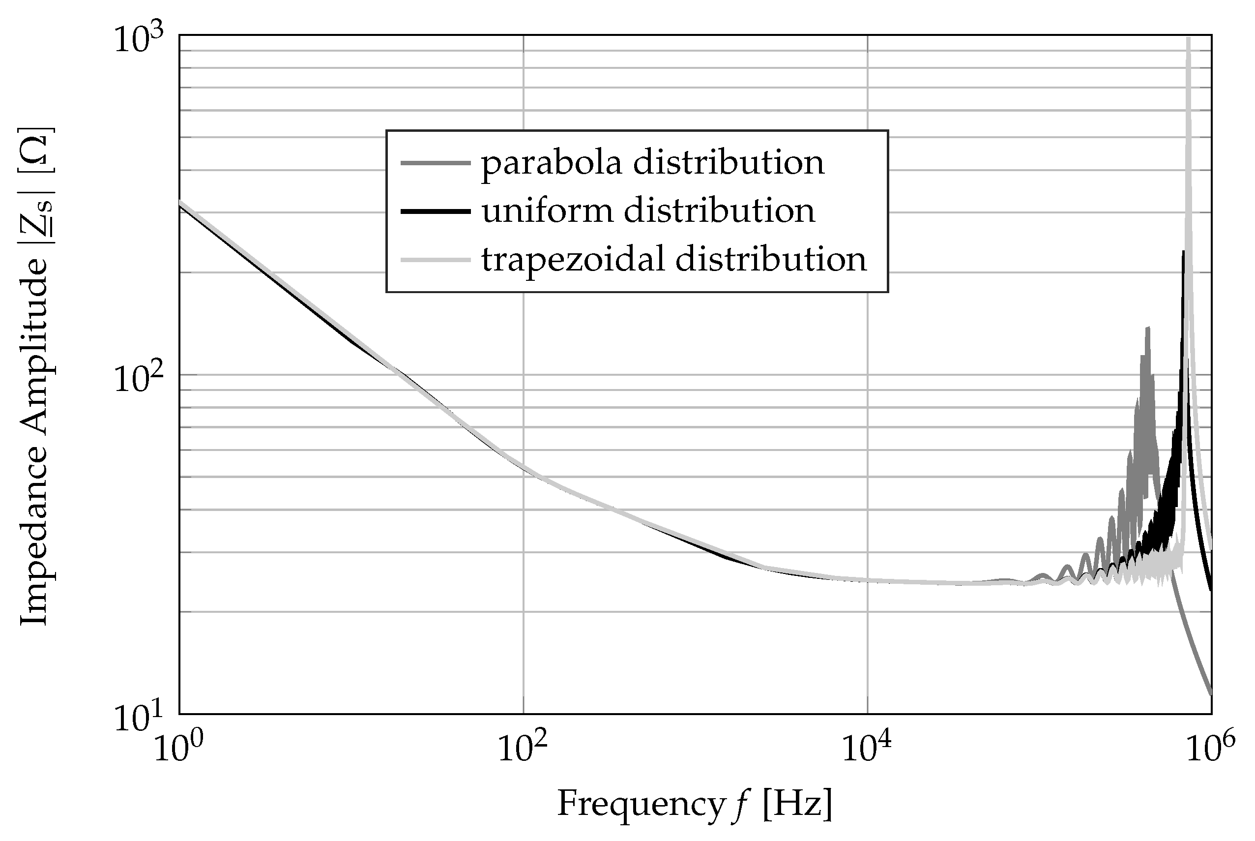
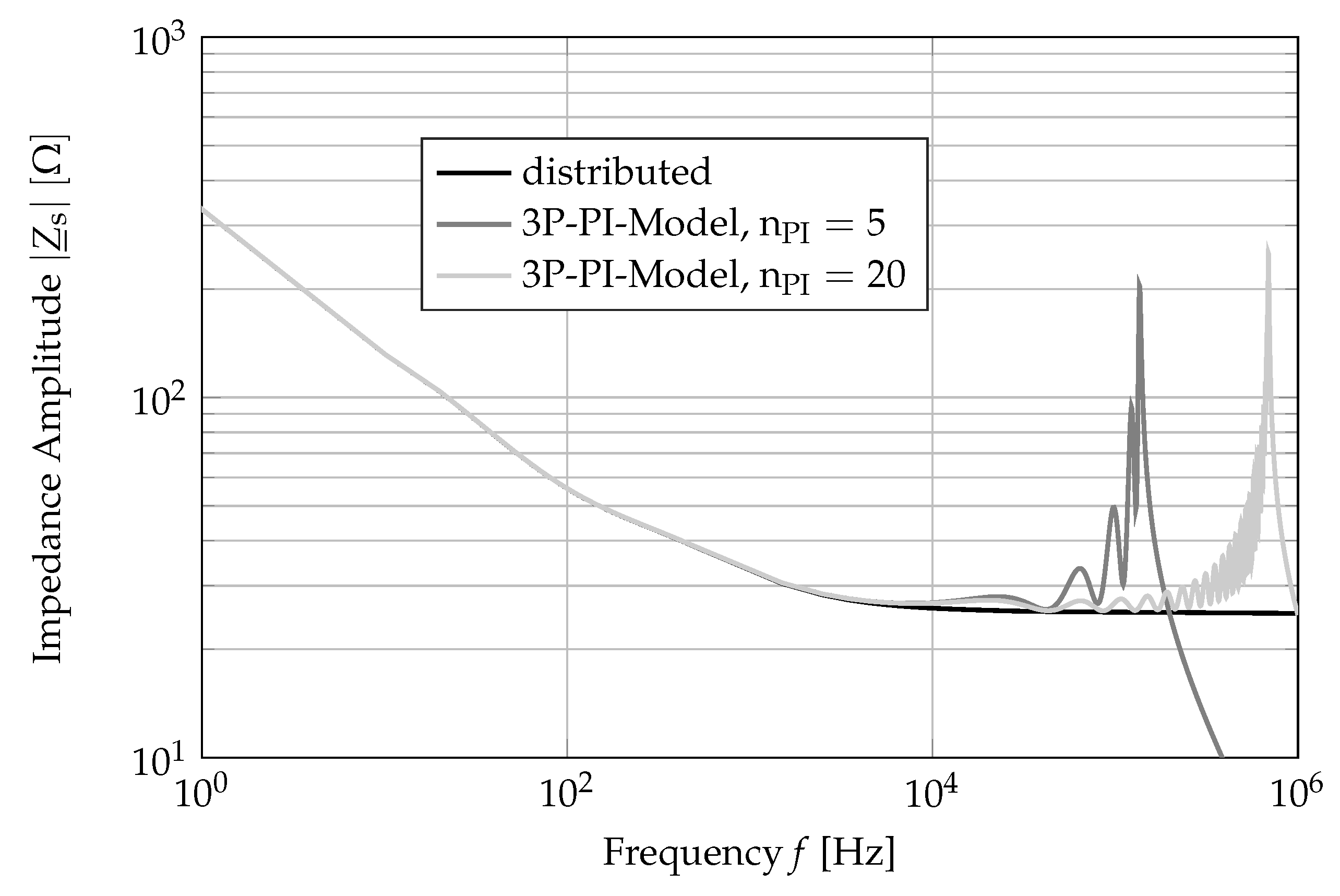
In this work, detailed investigations of the behavior of a previously developed 3P-PI-Model are introduced. It has been proven that the frequency dependence of cable parameters, the length distribution of PI-sections and the number of PI-sections impact the frequency and the amplitude of the main resonance of PI-sections.
In addition, the number of PI-sections has a big impact on the computational effort in the developed 3P-PI-Model. Using a large number of PI-sections increases the accuracy of the simulation results. On the other hand, the large number of PI-sections leads to a high computational effort.
Two algorithms to optimize the number of PI-sections are developed. In the first algorithm, an upper limit of the number of PI-sections is defined in order to limit the computational effort in the developed 3P-PI-Model.
In the second algorithm, the computational effort of the calculations in the developed 3P-PI-Model is reduced at the expense of the accuracy. To achieve this, the number of PI-sections is defined (starting from the upper limit of PI-sections) after specifying an error in the time delay.
A comparison of the outcomes of the developed 3P-PI-Model using the upper limit of PI-sections with measured data has shown a good match, which validates the approach used in the calculating of the number of PI-sections. In addition, a proper accuracy of the simulation results with a large reduction in the computational effort can be reached by specifying a small error in the time delay.
In this work, the proposed first and second algorithms are used to define the number of PI-sections for simulating of fast transients. However, both algorithms can also be used by different operating states of the power system (e.g., switching operations).


