Article

Solving Multi-Objective Fuzzy Optimization in Wireless Smart Sensor Networks under Uncertainty Using a Hybrid of IFR and SSO Algorithm

1
College of Mathematics and Informatics, South China Agricultural University, Guangzhou 510633, China
2
Integration and Collaboration Laboratory, Department of Industrial Engineering and Engineering Management, National Tsing Hua University, Hsinchu 300, Taiwan
3
Department of Industrial Management and Information, Southern Taiwan University of Science and Technology, Tainan 700, Taiwan
4
Department of Automation, Guangdong Polytechnic Normal University, Guangzhou 510633, China
5
Department of Logistics and Shipping Management, Kainan University, Taoyuan 33857, Taiwan
6
School of Mathematics, South China University of Technology, Guangzhou 510633, China
*
Author to whom correspondence should be addressed.
Energies 2018, 11(9), 2385; https://doi.org/10.3390/en11092385
Submission received: 20 July 2018 / Revised: 25 August 2018 / Accepted: 27 August 2018 / Published: 10 September 2018

Abstract

:
Wireless (smart) sensor networks (WSNs), networks made up of embedded wireless smart sensors, are an important paradigm with a wide range of applications, including the internet of things (IoT), smart grids, smart production systems, smart buildings and many others. WSNs achieve better execution efficiency if their energy consumption can be better controlled, because their component sensors are either difficult or impossible to recharge, and have a finite battery life. In addition, transmission cost must be minimized, and signal transmission quantity must be maximized to improve WSN performance. Thus, a multi-objective involving energy consumption, cost and signal transmission quantity in WSNs needs to be studied. Energy consumption, cost and signal transmission quantity usually have uncertain characteristics, and can often be represented by fuzzy numbers. Therefore, this work suggests a fuzzy simplified swarm optimization algorithm (fSSO) to resolve the multi-objective optimization problem consisting of energy consumption, cost and signal transmission quantity of the transmission process in WSNs under uncertainty. Finally, an experiment of ten benchmarks from smaller to larger scale WSNs is conducted to demonstrate the effectiveness and efficiency of the proposed fSSO algorithm.

1. Introduction

Wireless (smart) sensor networks (WSN) consist of smart sensors deployed and operated in wireless sensor networks, and have rapidly become an important design widely applied in many modern applications, such as the Internet of Things (IoT) [1,2], smart grids [3], healthcare and medical systems [4], wind energy systems [5], industrial automation [6], the smart transportation industry [7,8], the semiconductor industry [9] and smart cities [10]. The signal, information or flow cannot be successfully transmitted through the nodes, which are the sensors in the WSN, if the operation of the WSN system fails because nodes deplete their limited battery power. In other words, a critical restriction in any WSN system is energy consumption. Therefore, numerous investigations of WSNs have had a primary focus on energy consumption.
Optimizing energy efficiency (EE) in a WSN, which is defined as the ratio of output over energy consumption, has been the subject of a great number of studies. Mekonnen et al. [2] proposed a prototype of a WSN applied in a video surveillance system to optimize energy consumption. Trapasiya and Soni [11] addressed the goal of retransmission energy reduction in WSNs. Quang and Kim [12] proposed a gradient routing in an industrial WSN to optimize energy consumption. Setiawan et al. [13] came up with an energy management policy to maximize energy transfer efficiency for a WSN. Liu et al. [14] optimally designed a WSN to minimize energy consumption.
The minimization of energy consumption in WSNs has also been investigated by many researches [15,16,17,18]. Chanak et al. [19] discussed the balance of energy consumption among deployed sensors in a WSN. The energy-optimal routing problem in WSNs has recently been studied by several works [20,21,22]. The improvement of energy consumption by clustering method in a WSN has also been discussed by some works [23,24].
However, the measured values of energy consumption in real-life WSN systems are usually uncertain and imprecise. Fuzzy set theory can effectively resolve these uncertain and imprecise problems. In studies of energy consumption for WSNs, few researchers have presented fuzzy-based methods to solve uncertainty problems in such systems. Collotta et al. [25] considered the turning on/off of devices as the output of a Fuzzy Logic Controller (FLCs) because of the dynamical characteristics of the calculated distance from sensor nodes with regard to the Access Points (APs). They used a fuzzy-based technique to decide whether Wi-Fi access points should be switched off when they were underutilized to optimize the energy consumption of a WSN applied in a multimedia system. Kumar and Chaturvedi [26] considered the query dynamic, including the volume of the generated query, frequency of the query generation and the geographical distribution of the query, and aimed to optimize the energy efficiency in a WSN by treating the impact of uncertainties in the query generation process by a fuzzy method. Akram and Cho [27] considered the uncertainty of security attacks on sensor nodes, and adopted a fuzzy-based selection of the intermediate verification nodes for a WSN to optimize energy consumption. Also, there are many other recent work which have considered parameter optimization in WSN and the details can be found in [28,29,30].
In this study, a fuzzy-based algorithm is adopted to solve the uncertain characteristics of energy consumption in a WSN. A schematic picture of a WSN is provided in Figure 1, in which sensor nodes are expressed as circles in the WSN. Let the target sensor node represent the source node. Many paths can be chosen to transmit a signal from the source node to the sink node each node is expressed as a circle in Figure 1. For example, one chosen path sends the signal from the source node to the sink node through two linking sensor nodes which are dark colored in Figure 1.
To the best of the authors’ knowledge, this is the first work to use a fuzzy-based algorithm to effectively resolve uncertain problems of energy consumption measurement in a WSN system. In addition, arcs are used to represent the transmission process among the sensors in a WSN so that an activity on arcs (AOA) network can be implemented. This work, therefore, suggests a fuzzy-based algorithm to resolve the uncertain problems of energy consumption measurements in a WSN using an AOA network. Moreover, fuzzy cost and fuzzy signal transmission quantity are also considered in the proposed algorithm to enhance performance of the WSN system. Finally, an experiment is conducted to demonstrate that the proposed fuzzy-based algorithm can significantly and efficiently optimize WSN energy consumption.
The uncertain characteristics of energy consumption, cost and signal transmission quantity are briefly described as follows. Assume that Figure 2 is a WSN with the nodes set: {0, 1, 2, 3} and the arcs set: {a1, a2, a3, a4, a5, a6}. Node 0 and node 3 are the source node and sink node, respectively. Arcs a1, a2, a4, a5 and a6 are designed as the directed arcs. Therefore, there are 4 paths (alternatives): P1 = {0, 1, 3}, P2 = {0, 2, 3}, P3 = {0, 1, 2, 3} and P4 = {0, 2, 1, 3}, which transmit signal from the source node to the sink node. The related information of fuzzy energy consumption, fuzzy cost and fuzzy signal transmission quantity of sensors in Figure 2 are presented in Table 1.
As mentioned in the above discussion, a new multi-objective fuzzy problem arises involving three objectives: energy consumption, cost and signal transmission quantity in WSNs. Hence the goal of the proposed problem is to find a path, say path i, such that total utility value U(i) (see Equation (24) in Section 3.1) is maximal in sending signal between a pair of nodes under uncertainty, e.g., the change of the topologies, the changes in nodes’ energetic levels, sensor breakdowns, etc. in WSNs.
Since the 1990s, various forms of artificial intelligence have been applied to different optimization NP-problems which mean the running time increases dramatically as the number of nodes in the networks increases. [6,7,8,9,10,11,12,13,14,15,16,17,18,19,20,21,22,23,24,25,26,27,31,32,33,34,35,36,37,38]. For example, genetic algorithms [39], artificial bee colony algorithms [40], particle swarm optimization [34,37,41,42], simplified swarm optimization (SSO) [34,35,36,37,38,42,43,44,45], grey wolf [46], neural network [13,41,45,47], harmony search algorithm [47], Sugeno-Type Fuzzy Inference [48], etc. Among these algorithms, SSO proposed by Yeh is the most simple one. Also, Yeh’s SSO is most customizable amongst other algorithms to apply and solve relevant [34]. Hence, SSO is adapted here to create a fuzzy-based SSO to solve the proposed fuzzy optimization NP-problem.
The remainder of this paper is structured as follows. Section 2 introduces the fundamentals of fuzzy set theory, including arithmetic operations of fuzzy numbers, fuzzy criteria matrix with its addition as well as maximizing set and minimizing set. Section 3 introduces the inverse function-based fuzzy ranking (IFR) and simplified swarm optimization (SSO), which are the basis of the proposed algorithm. Numerical examples for these two methods are provided. The proposed fuzzy SSO (fSSO) for solving a WSN problem is presented in Section 4, and Section 5 examines the performance of the proposed algorithm. Conclusions and suggestions for future research are offered in Section 6.

2. Fuzzy Set Theory and the Proposed Fuzzy Criteria Matrix

Fuzzy set theory was first introduced by Zadeh in 1965 [31], and has become a popular and efficient method for solving uncertain and imprecise problems in decision-making. The fundamental concepts and the proposed Fuzzy criteria matrix are presented in this section.

2.1. Fuzzy Set and Arithmetic Operations

The XXXXX definitions of fuzzy set, α-cuts of a fuzzy set, triangular fuzzy number and arithmetic operations on fuzzy numbers are introduced below.
Definition 1.
A fuzzy set A is defined in Equation (1), where U denotes the universal discourse, x is a real number, −∞ ≤ x ≤ ∞, and uA represents membership function of the fuzzy set. Let x be a number allocated to A. A corresponding real number can be found for the membership function of the fuzzy set uA(x) belonging to [0,1], i.e., 0 ≤ uA(x) ≤ 1 [49]:
A = {(x, uA(x)) | xU}
Definition 2.
The α-cuts of a fuzzy set A are defined in Equation (2), where Aαa and Aαd are the lower bound and the upper bound of the α-cut, respectively:
Aα = {(x, uA(x) ≥ α) | xU} = [Aαa, Aαd]
Definition 3.
A = (a, b, c), where a ≤ b ≤ c, is a triangular fuzzy number and can be defined as in Equation (3) and depicted in Figure 3:
u A ( x ) = { ( x a ) / ( b a ) , a x b , ( x c ) / ( b c ) , b x c , 0 , otherwise ,  
Definition 4.
Suppose two triangular fuzzy numbers A1 = (a1, b1, c1) and A2 = (a2, b2, c2), the standard operations on triangular fuzzy numbers are as shown in Equations (4)–(7):
Fuzzy addition: A1A2 = (a1 + a2, b1 + b2, c1 + c2)
Fuzzy subtraction: A1ΘA2 = (a1c2, b1b2, c1a2)
Fuzzy multiplication: A1A2 = (a1 × a2, b1 × b2, c1 × c2)
Fuzzy division: A1A2 = (a1/c2, b1/b2, c1/a2)
The concept of Chen’s maximizing set and minimizing set (1985) is introduced in Definitions 5–6 below:
Definition 5.
Let M and H be the maximizing set and the minimizing set defined as Equations (8) and (9):
f M ( x ) = { [ x x min x max x min ] k x min x x max 0 otherwise ,
f H ( x ) = { [ x max x x max x min ] k x min x x max 0 otherwise  
where xmin = inf S, xmax = sup S, S = i = 1 n S i , Si = {x | f A i ( x ) >0}, and Ai is the fuzzy number of each alternative, i = 1, 2, …, n.
Suppose there are two fuzzy numbers A1 and A2. The maximizing set and minimizing set associated with A1 and A2 can be presented as shown in Figure 4.
Definition 6.
The right, left, and total utility value of alternative Ai are defined as UR(i) and UL(i) and U(i), respectively:
U R ( i )   =   sup x ( f M ( x ) f A i ( x ) ) ,   i   =   1 ,   2 ,   ,   n .
U L ( i )   =   sup x ( f H ( x ) f A i ( x ) ) ,   i   =   1 ,   2 ,   ,   n .
U(i) = UR(i) + UL(i)

2.2. The Proposed Fuzzy Criteria Matrix and Its Addition

The fuzzy criteria matrix is proposed to aggregate the three fuzzy criteria, energy consumption, cost and signal transmission quantity, into one matrix. In the fuzzy criteria matrix, each row represents the related criterion in a triangular fuzzy number. For example, in Figure 2, the fuzzy criteria matrix of sensor 1 is:
A 1 = [ 1 4 6 2 3 7 1 4 7 ] ,
where the ith row represents the related triangular fuzzy number of the ith criterion, i.e., (2, 3, 7) is the triangular fuzzy number of the cost of sensor 1.
Similarly, the fuzzy criteria matrices of sensors 2–6 can be displayed as:
A 2 = [ 1 3 5 2 4 5 2 3 5 ] , A 3 = [ 2 3 4 1 3 4 1 3 4 ] , A 4 = [ 1 2 4 1 3 7 1 2 7 ] , A 5 = [ 1 3 4 1 3 7 1 3 7 ] , A 6 = [ 1 4 5 2 4 7 2 4 7 ]  
By Equation (4), the fuzzy criteria matrix of each path or arc can be obtained as:
A 1 A 2 = [ 1 4 6 2 3 7 1 4 7 ] + [ 1 3 5 2 4 5 2 3 5 ] = [ 1 + 1 4 + 3 6 + 5 2 + 2 3 + 4 7 + 5 1 + 2 4 + 3 7 + 5 ] = [ 2 7 11 4 7 12 3 7 12 ] .
There are four paths (alternatives) in Figure 2, P1 = {0, 1, 3}, P2 = {0, 2, 3}, P3 = {0, 1, 2, 3} and P4 = {0, 2, 1, 3}, which transmit a signal from the source node to the sink node. Therefore, the fuzzy criteria matrices of these paths can be obtained using the proposed fuzzy criteria matrix addition as follows. For example, the matrix for P1 is obtained by the following procedure:
P 1 = A 1 A 5 = [ 1 4 6 2 3 7 1 4 7 ] + [ 1 3 4 1 3 7 1 3 7 ] = [ 2 7 10 3 6 14 2 7 14 ] .
Similarly, the fuzzy criteria matrix addition of paths P2, P3 and P4 can be produced as:
P 2 = A 2 A 6 = [ 1 3 5 2 4 5 2 3 5 ] + [ 1 4 5 2 4 7 2 4 7 ] = [ 2 7 10 4 8 12 4 9 12 ]  
P 3 = A 1 A 4 A 6 = [ 1 4 6 2 3 7 1 4 7 ] + [ 1 2 4 1 3 7 1 2 7 ] + [ 1 4 5 2 4 7 2 4 7 ] = [ 3 10 15 5 10 21 4 10 21 ]  
P 4 = A 2 A 3 A 5 = [ 1 3 5 2 4 5 2 3 5 ] + [ 2 3 4 1 3 4 1 3 4 ] + [ 1 3 4 1 3 7 1 3 7 ] = [ 4 9 13 4 10 16 4 9 16 ] .

3. The IFR, SSO and the Proposed Fitness Function

A multi-criteria multi-objective fuzzy optimization problem is considered in this work. In optimization problems, it is very important to solve for the best among all solutions regardless of the environment being certain or uncertain.
Chu and Yeh’s inverse function-based fuzzy number ranking method (IFR) is able to transform fuzzy numbers from a fuzzy multi-criteria decision-making model into crisp numbers [32]. Their method is more robust compared with some others. Meanwhile, Yeh’s simplified swarm optimization (SSO) is more easily customized to solve relevant problems than other algorithms [34]. Herein, an algorithm that combines the IFR and the SSO is used to solve the proposed problem. The methods of IFR and SSO, along with examples are presented in the following subsections, respectively. Moreover, the proposed fitness function based on the IFR is discussed.

3.1. The Inverse Function-Based Fuzzy Number Ranking

Assume that n alternatives P1, P2, …, Pn are required to be evaluated under n criteria F1, F2, …, Fn of which F1, F2, …, Fg are benefit criteria, and the rest are cost criteria. In IFR, each alternative, Pi, is represented by a triangular fuzzy number, ξi,j = (αi,j, βi,j, χi,j), for each criterion j. Fuzzy number ξi,j must be normalized to Xi,j = (ai,j, bi,j, ci,j), of which values of elements in Xi,j fall into [0,1], and can be weighted by multiplying the weight Wj = (wj,1, wj,2, wj,3) in order to obtain the fuzzy weighted normalized evaluation value Gi = (Ai, Bi, Ci) for each alternative. Note that the multiplication of two triangular fuzzy numbers can be approximated as a triangular fuzzy number. Hence, the fuzzy number Gi is still a triangular fuzzy number, where i = 1, 2, …, n; j = 1, 2, …, m.
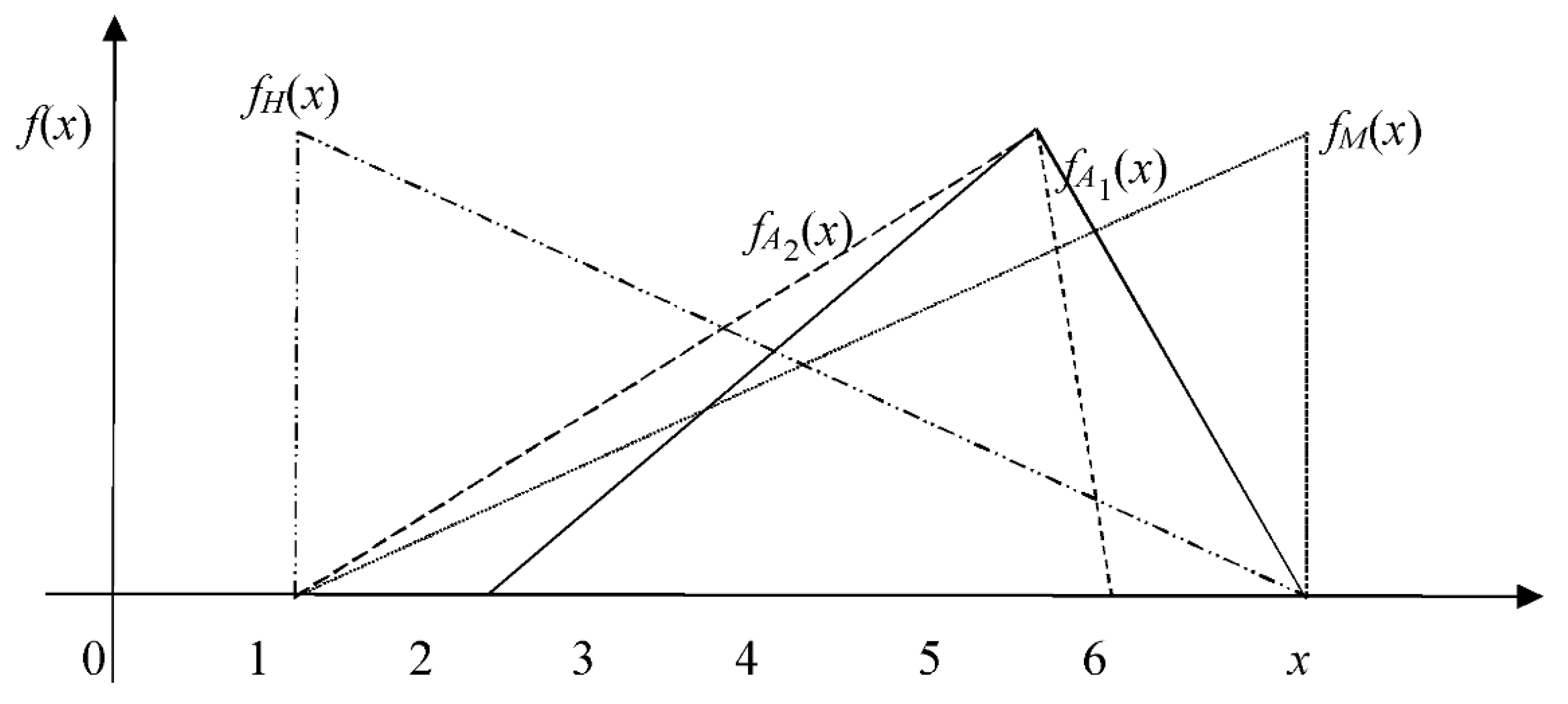
The right utility UR(i) of Pi is obtained from the right inverse function yRi of Gi and the inverse function of the maximizing set fM(x); while the left utility UL(i) of Pi is obtained from the left inverse function yLi of Gi and the inverse function of the minimizing set fH(x). The total utility U(i) is the sum of UR(i) and UL(i). A larger U(i) indicates that the corresponding alternative Ai is more favorable than the others. The procedure of IFR is described in the following steps [32]:
Step F0.
Find the weight Wj = (wj,1, wj,2, wj,3) of criterion j, j = 1, 2, …, m.
Step F1.
Normalize the triangular fuzzy number of each alternative versus each criterion, ξi,j = (αi,j, βi,j, χi,j), i = 1, 2, …, n; j = 1, 2, …, m, to Xi,j = (ai,j, bi,j, ci,j) to make evaluation values across criteria in a comparable scale. Herein Equation (20) is used for normalization [32,33]:
X i , j = ( α i , j min   i α i , j max   i χ i , j min   i α i , j ,   β i , j min   i α i , j max   i χ i , j min   i k i , j ,   χ i , j min   i α i , j max   i χ i , j min   i k i , j ) .
Step F2.
Calculate the weighted normalized triangular fuzzy number Gi,j = (Ai,j, Bi,j, Ci,j) = (ai,jwi,1, bi,jwi,2, ci,jwi,3) and the aggregated triangular fuzzy number Gi = (Ai, Bi, Ci) for alternative i, i = 1, 2, …, n, as shown in Equation (21):
G i =   ( A i , B i , C i )   = j = 1 g ( W j X i , j ) j = g + 1 n ( W j X i , j ) ,
where Gi = Gi,1 + Gi,2Gi,3; Ai = Ai,1 + Ai,2Ai,3; Bi = Bi,1 + Bi,2Bi,3; Ci = Ci,1 + Ci,2Ci,3.
Step F3.
Calculate the right inverse function yRi and the left inverse function yLi as shown in Equations (22) and (23):
UR(i) = (Cixmin)/(xmaxxminBi + Ci)
UL(i) = (Aixmax)/(xminxmaxBi + Ai).
Step F4.
Calculate total utility value U(i) of alternative i based on Equation (12) for i = 1, 2, …, n:
U(i) = (BiCi)∙UR(i) + (BiAi) UL(i) + Ci + Ai.
Step F5.
Find the best alternative which has the largest inverse function-based total utility value. The flow chart of the above algorithm is depicted in Figure 5:

3.2. The SSO and an Example

The proposed fSSO is developed based on the SSO. In 2009, Yeh first developed the SSO algorithm, initially called discrete PSO, to overcome the weakness of particle swarm optimization (PSO) in solving discrete problems [34]. Since then, the SSO has become a famous swarm intelligence-based random optimization algorithm. The SSO has also played a very significant solution role in relevant studies of artificial intelligence. Furthermore, the SSO has been applied by many papers to solve different types of problems in various fields [35,36,37,38,43].
The parameters cg, cp, cw and cr are the probabilities of the new variable value generated from a global search, a global search together with a local search, a local search, and a random number in SSO, respectively, where cg + cp + cw + cr = 1. The update mechanism of the simple, efficient and agile SSO algorithm is presented as Equation (25):
x t , i , j = { p g B e s t , j p i , j x t 1 , i , j x if   ρ [ 0 , C g )   if   ρ [ C g , C p ) if   ρ [ C p , C w ) if   ρ [ C w ,   1 ] ,
where the number of generations is denoted as t, t = 1, 2, …, Ngen; the number of solutions is denoted as i, i = 1, 2, …, Nsol; the number of variables is denoted as j, j = 1, 2, …, Nvar; xt,i,j and xt−1,i,j are the ith solution of the jth variable at generations t and t − 1, respectively; PgBest,j and Pi,j are the jth variable of the temporary global best of all solutions and the temporary personal (local) best of the ith solution, respectively; ρ belongs to uniform distribution [0,1]; Cg = cg, Cp = Cg + cp, Cw = Cp + cw; x belongs to uniform distribution [li, ui].
Let Cg = cg = 0.5, Cp = Cg + cp = 0.5 + 0.2 = 0.7, Cw = Cp + cw = 0.7 + 0.25 = 0.95, X10,8 = (1.1, 1.8, 3.5, 2.2, 0.1) which is the 8th solution of the 11th generation, P8 = (2.5, 2.0, 1.2, 1.9, 5.0), and PgBest = (3.3, 2.8, 1.2, 4.5, 5.6). An example is shown below to explain how SSO is implemented to update X10,8 to X11,8 in Table 2. The lower bound li, the upper-bound ui, and the value of ρi for variable x10,8,i are listed in the 2nd, 3rd and 7th row of Table 2, respectively.

3.3. The Proposed Fitness Function

In IFR, all alternatives (i.e., all paths here) are represented by fuzzy numbers and these fuzzy numbers must be normalized to a comparable scale. The normalization procedure is conducted using maximal and minimal elements among those alternatives versus each criterion. However, each alternative is updated from generation to generation, i.e., the maximal and minimal elements among alternatives in generation i may be different to those in generation j for all i < j. The above situation means that in the gBest in generation i is not better than some solutions in generation j after using the new maximal and minimal elements obtained from generation j. This is contrary to the meaning of gBest.
To fix the above problem, both the minimal xmin and the maximal xmax are redefined by the following equations:
x min = min i { a i , j }  
x max = max i { c i , j }  
where i = 1, 2, …, n and j = 1, 2, …, m. The values of xmin and xmax are always fixed and all fitness values of solutions are also fixed after the redefinition.
Example 1.
Suppose three criteria including energy consumption, cost and signal transmission quantity are considered in Figure 2, and are denoted by symbol j = 1, 2, 3.
Solution:
Step F0.
The triangular fuzzy weight, denoted as Wj = (wj,1, wj,2, wj,3) obtained from the analytic hierarchy process (AHP) for each criterion j, j = 1, 2, 3, is provided as shown in Table 3:
Step F1.
By the addition of the fuzzy criteria matrix presented in Section 2.2, triangular fuzzy values of the paths (i.e., alternatives): P1 = {0, 1, 3}, P2 = {0, 2, 3}, P3 = {0, 1, 2, 3} and P4 = {0, 2, 1, 3} versus different criteria can be shown as in Table 4:
The values of min   i α i , j and max   i χ i , j for each criterion are indicated in bold and underlined in Table 3, respectively, and are presented in Table 5:
By Equation (20), normalize triangular fuzzy numbers Xi,j = (ai,j, bi,j, ci,j) for paths (alternates), i = 1, 2, 3, 4, versus criteria, j = 1, 2, 3, can be obtained as presented in Table 6:
Step F2.
Values of Gi,j = (Ai,j, Bi,j, Ci,j), i = 1, 2, 3, 4 and j = 1, 2, 3, can be obtained by (Ai,j, Bi,j, Ci,j) = (ai,jwi,1, bi,jwi,2, ci,jwi,3) as shown in Table 7. Values of Gi = (Ai, Bi, Ci) can be obtained from Equation (21) as listed in Table 8:
Step F3.
The right inverse function UR(i) and the left inverse function UL(i) based on Equations (22) and (23) can be produced as shown in Table 9:
Step F4.
The inverse function-based total utilities U(i) of alternatives are listed in Table 10:
Step F5.
From Table 10, it is clear that path P1 is the best transmission path because it has the lowest total utility value, i.e., U(1) < U(2) < U(4) < U(3).

4. The Proposed Fuzzy SSO

The proposed fSSO is a population, all-variable and stepwise-function-based soft computing method, i.e., there are a fixed number of solutions in each generation and all variables must be updated based on the stepwise function with each solution.

4.1. The Flexible-Length Structure without Targets Solution Structure

Each solution in the proposed fSSO is a path, which records a sequence of nodes from the source node to the sink node, and is also called an alternative in the multi-criteria decision-making problem. For example, both P1 = (0, 1, 3) and P2 = (0, 1, 2, 3) are paths from nodes 0 to 3 in Figure 2.
The lengths of all paths are different, e.g., there are two and three arcs in P1 and P2, respectively. Herein, the flexible-length solution structure is used. In addition, only non-target nodes are recoded sequentially in each solution to save memory space and processing time. For example, P1 = (0, 1, 3) and P2 = (0, 1, 2, 3) in Figure 2 can be simplified to P1 = (1) and P2 = (1, 2) without showing the source and sink nodes. Note that the processing time and the memory space can be reduced by up to (2/Nvar)∙Nsol∙Ngen and (2/Nvar) times of those results without using this concept, respectively.

4.2. The Novel Update Mechanism

The proposed fSSO has a fixed population in each generation and all variables of each solution must be updated based on the stepwise function, which is based on the original stepwise function listed in Equation (25), and is modified to fit the proposed problem as follows:
x i , j = { p g B e s t , j p i , j x i , j x if   ρ [ 0 , 1 ] [ 0 , C g )   and   j < X g B e s t if   ρ [ 0 , 1 ] [ C g , C p )   and   j < P i if   ρ [ 0 , 1 ] [ C p , C w ) if   ρ [ 0 , 1 ] [ C w ,   1 )  
where ρ [ 0 , 1 ] is the same as that defined in Equation (25) and X < Nvar is defined to be the length of X, e.g., the number of variables in X. Note that the length of the new update Xi is 20% longer than the longest among old Xi before it is modified to be a feasible solution. For example, let X5 = (2, 4, 6, 8, 10), P5 = (1, 3, 5, 7) and PgBest = G = (5, 2, 7, 4, 6, 3, 1). The new length of the new X5 is set to the smallest integer that is larger than 7 · (1 + 20%) = 8.5, i.e., 9 since P 5 = 4 < X 5 = 5 < G = 7 . Assume Cg = 0.35, Cp = 0.55, Cw = 0.65, ρ = (ρ1, ρ2, …, ρ9) = (0.3, 0.5, 0.1, 0.5) for this X5. From Equation (28), the process to update X5 is displayed in Table 11.

4.3. The Solution Repair Procedure

From the example shown in Section 4.2, the obtained solutions may have duplicated nodes, e.g., 5 appears in the first and seventh coordinates of the new X5. Any solution with duplicate nodes is infeasible. Hence, duplicate nodes must be removed randomly to repair an infeasible solution to a feasible solution, which represents a simple routing. For example, the new X5 = (5, 3, 7, 8, 6, 2, 5, 7, 1), and it can be (3, 8, 6, 2, 5, 7, 1), (5, 3, 7, 8, 6, 2, 5, 1), (5, 3, 7, 8, 6, 2, 1) or (5, 3, 8, 6, 2, 7, 1) after the repair.

4.4. The Pseudo Code and Flowchart of the Proposed fSSO

The details of fSSO are described in the following steps, and the flowchart of fSSO is depicted in Figure 6.
Step 0.
Generate X0,i = Pi randomly, calculate U(X0,i), find gBest, and let t = 1, where i = 1, 2, …, Nsol.
Step 1.
Let i = 1.
Step 2.
Update Xi based on the above equation, repair Xi if possible, and calculate U(Xt,i).
Step 3.
If U(Xi) is better than U(Pi), then let Pi = Xi. Otherwise, go to Step 5.
Step 4.
If U(Pi) is better than U(PgBest), then let gBest = i.
Step 5.
If i < Nsol, let i = i + 1 and go to Step 2.
Step 6.
If t < Ngen, then let t = t + 1 and go back to Step 1. Otherwise, halt.

5. Numerical Experiments

The proposed fSSO for this problem is only run immediately once a signal request for any pair of nodes to overcome the uncertainty is received. The answer obtained from the proposed algorithm thus corresponds to the real-life and real-time WSNs under uncertain environment and situations including sensor breakdowns, the change of network topology, the changes in nodes’ energetic levels and the network topologies, etc.

5.1. Experimental Setting and Metrics Derivation

To verify the performance of the proposed fSSO, the fSSO are compared with SSO [34] and Ant colony optimization (ACO) algorithms [30] by two metrics following.
  • Statistical analyses of the minimum, maximum, average and standard deviation of the fitness values.
  • Statistical analyses of the minimum, maximum, average and standard deviation of the running time.
The proposed fSSO, SSO [34] and ACO [30] are coded using DEV C++ with 64-bit Windows 10, implemented on an Intel Core i7-6650U CPU @ 2.20 GHz 2.21 GHz notebook with 64 GB memory. The proposed fSSO, SSO [34] and ACO [30] are executed on ten benchmarks including Nvar = 100, 200, 300, 400, 500, 600, 700, 800, 900 and 1000 sensor nodes in the WSN, respectively. The number of runs, generations, and solutions of each benchmark are equal to 30, 100, and 50, respectively, i.e., Nrun = 30, Ngen = 100, and Nsol = 50 for three algorithms. After the process of trial and error, the parameters of the proposed fSSO and SSO [34] are Cg = 0.35, Cp = 0.55, and Cw = 0.65, i.e., cg = 0.35, cp = 0.20, cw = 0.10, and cr = 0.35. The parameters of ACO are adapted from [30]. The related performance includes the fitness values of the inverse function-based total utility values described in Equation (28).

5.2. Analysis of Results

Statistical analyses of the minimum, maximum, average and standard deviation of the fitness values from the ten benchmarks are displayed in Figure 7, Figure 8, Figure 9 and Figure 10, where the y-axis and x-axis are the related fitness values and the number of sensors Nvar, respectively. The best solutions, e.g., U(PgBest), of the minimum, maximum, average and standard deviation among the ten benchmarks are indicated in bold in Table 12, Table 13, Table 14 and Table 15, respectively.
From Table 12, Table 13, Table 14 and Table 15, performance of the proposed fSSO compared with SSO and ACO in the WSN is concluded as follows:
  • The proposed fSSO possesses the ability to solve multi-objective problems in a WSN.
  • The proposed fSSO can be applied to not only small scale problems involving 100 sensor nodes, but also big scale problems involving 1000 sensor nodes in a WSN.
  • The proposed fSSO can effectively find the best configuration of the number of sensor nodes in a WSN.
  • According to Table 12, the configuration of 500, 800 and 900 sensor nodes in a WSN has the best solutions of minimum fitness values obtained by the proposed fSSO compared with those found by SSO and ACO for the proposed multi-objective problem including energy consumption, cost and signal transmission quantity.
  • According to Table 13, Table 14 and Table 15, the configuration of ten benchmarks of 100, 200,…, 1000 sensor nodes in a WSN has the best solutions of maximum, average and standard deviation of fitness values obtained by the proposed fSSO compared with those found by SSO and ACO for the proposed multi-objective problem including energy consumption, cost and signal transmission quantity.
Moreover, statistical analyses of the minimum, maximum, average and standard deviation of the running time from the ten benchmarks are displayed in Figure 11, Figure 12, Figure 13 and Figure 14, where the x-axis and y-axis are the related running times based on CPU seconds for each benchmark. The best solutions of the minimum, maximum, average and standard deviation among the ten benchmarks are indicated in bold in Table 16, Table 17, Table 18 and Table 19. From Table 16, Table 17, Table 18 and Table 19, performance of running time obtained by the proposed fSSO compared with those found by SSO and ACO in the WSN is concluded as follows:
  • According to Table 16 and Table 17, the configuration of ten benchmarks of 100, 200,…, 1000 sensor nodes in a WSN has the best solutions of minimum and maximum running time obtained by either the proposed fSSO or ACO compared with those found by SSO for the proposed multi-objective problem including energy consumption, cost and signal transmission quantity.
  • According to Table 18, the configuration of 100, 200, 300 and 400 sensor nodes in a WSN has the best solutions of average running time obtained by the proposed fSSO compared with those found by SSO and ACO for the proposed multi-objective problem including energy consumption, cost and signal transmission quantity. And the configuration of 500, 600, …, 1000 sensor nodes in a WSN has the best solutions of average running time obtained by ACO.
  • According to Table 19, the configuration of 400, 500 and 1000 sensor nodes in a WSN has the best solutions of standard deviation running time obtained by ACO compared with those found by SSO and the proposed fSSO for the proposed multi-objective problem including energy consumption, cost and signal transmission quantity. And the configuration of 100, 200, 300, 600, 700, 800 and 900 sensor nodes in a WSN has the best solutions of standard deviation running time obtained by the proposed fSSO.

6. Conclusions

Optimization of the transmission process with respect to a multi-objective of energy consumption, cost and signal transmission quantity in a WSN was studied in this paper. The sensor nodes are usually set up in remote, inaccessible or hazardous environments, which be negatively affected by various external factors such as heavy rain, sunlight, wind, snow and earthquake etc., and this may result in uncertainty of energy consumption, cost and signal transmission quantity of the sensor nodes in a WSN. To resolve the problems of uncertainty and ranking of transmission paths in consideration of the multi-objective of energy consumption, cost and signal transmission quantity in a WSN, a fuzzy simplified swarm optimization algorithm (fSSO) is proposed. To the best of the authors’ knowledge, this is the first work which effectively resolves the uncertainty problems of energy consumption, cost and signal transmission quantity in a WSN using a fuzzy-based algorithm.
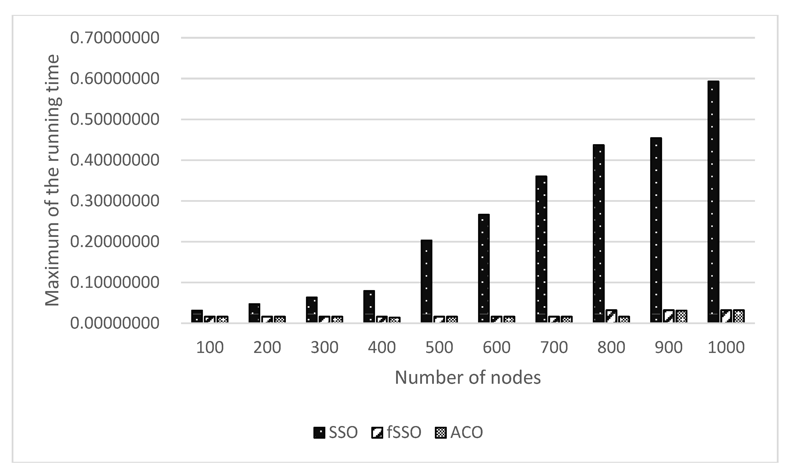
The methods of inverse function-based fuzzy number ranking (IFR) and SSO were applied to the proposed fSSO algorithm to defuzzify the fuzzy characteristics of the problem, and to transform the multi-objective problem into a single objective problem in order to solve optimization in the WSN. Furthermore, two rising operators including the flexible-length structure without targets solution structure and a novel SSO update mechanism were introduced to the developed fSSO algorithm. An experiment of ten benchmarks from smaller scale to larger scale including 100, 200, 300, 400, 500, 600, 700, 800, 900 and 1000 sensor nodes in a WSN was successfully conducted to demonstrate the effectiveness and efficiency of the proposed fSSO algorithm. When compared with the SSO [31] and ACO [49], the proposed fSSO algorithm shows the improvement in solution quality. For future studies, more objectives of the transmission process in the WSN by the proposed fSSO algorithm, the energy used in diverse computations (e.g., data aggregation, data compression, encryption, etc.), and the effects of the random parameters in the algorithms, will all be taken into account.

Author Contributions

The conceptualization, methodology and software are completed by M.W. and W.-C.Y.. M.W., W.-C.Y., and T.-C.C. have done the job of validation. The formal analysis is done by M.W., W.-C.Y., T.-C.C., X.Z., and C.-L.H. M.W., W.-C.Y., T.-C.C., X.Z., C.-L.H., and J.Y. all contribute in the writing-original draft preparation and writing-review & editing. The visualization and supervision are directed by M.W. and W.-C.Y. W.-C.Y. instructs the project administration. M.W. responses the funding acquisition.

Funding

This research was funded by Ministry of Science and Technology (Taiwan) grant number MOST 104-2221-E-007-061-MY3 and MOST 107-2221-E-007-072-MY3; National Natural Science Foundation of China grant number 61202269, 61472089, 61202293, and 31600591; Science and Technology Plan Project of Guangdong Province grant number 2014A050503057, 2015A020209124, 2016A020210087, and 2017A010102013; Science Foundation of Guangdong Province grant number 2015A030310180.

Acknowledgments

We wish to thank the anonymous editor and the referees for their constructive comments and recommendations, which have significantly improved this paper. This research was supported in part under grant MOST 104-2221-E-007-061-MY3 and MOST 107-2221-E-007-072-MY3.

Conflicts of Interest

The authors declare no conflict of interest.

References

  1. Chu, Z.; Zhou, F.; Zhu, Z.; Hu, R.Q.; Xiao, P. Wireless powered sensor networks for internet of things: Maximum throughput and optimal power allocation. IEEE Int. Things J. 2018, 5, 310–321. [Google Scholar] [CrossRef]
  2. Mekonnen, T.; Porambage, P.; Harjula, E.; Ylianttila, M. Energy consumption analysis of high quality multi-tier wireless multimedia sensor network. IEEE Access 2017, 5, 15848–15858. [Google Scholar] [CrossRef]
  3. Shehadeh, H.A.; Idris, M.Y.I.; Ahmedy, I.; Ramli, R.; Noor, N.M. The multi-objective optimization algorithm based on sperm fertilization procedure (MOSFP) method for solving wireless sensor networks optimization Problems in smart grid applications. Energies 2018, 11, 97. [Google Scholar] [CrossRef]
  4. Dey, N.; Ashour, A.S.; Shi, F. Developing residential wireless sensor networks for ECG healthcare monitoring. IEEE Trans. Consum. Electron. 2017, 63, 442–449. [Google Scholar] [CrossRef]
  5. Kosunalp, S. An energy prediction algorithm for wind-powered wireless sensor networks with energy harvesting. Energy 2017, 139, 1275–1280. [Google Scholar] [CrossRef]
  6. Cenedese, A.; Luvisotto, M.; Michieletto, G. Distributed clustering strategies in industrial wireless sensor networks. IEEE Trans. Ind. Inform. 2017, 13, 228–237. [Google Scholar] [CrossRef]
  7. Gao, M.; Wang, P.; Cao, Y.; Chen, R.; Cai, D. Design and verification of a rail-borne energy harvester for powering wireless sensor networks in the railway industry. IEEE Trans. Intell. Transp. Syst. 2017, 18, 1596–1609. [Google Scholar] [CrossRef]
  8. Friesen, M.; Jacob, R.; Grestoni, P.; Mailey, T.; Friesen, M.R.; McLeod, R.D. Vehicular traffic monitoring using bluetooth scanning over a wireless sensor network supervision de la circulation automobile en utilisant un balayage bluetooth à travers un réseau de capteurs sans fils. Can. J. Electr. Comput. Eng. 2014, 37, 135–144. [Google Scholar] [CrossRef]
  9. Colins, K.; Li, L.; Liu, Y. Analysis of a statistical relationship between dose and error tallies in semiconductor digital integrated circuits for application to radiation monitoring over a wireless sensor network. IEEE Trans. Nucl. Sci. 2017, 64, 1151–1158. [Google Scholar] [CrossRef]
  10. Csáji, B.C.; Kemény, Z.; Pedone, G.; Kuti, A.; Váncza, J. Wireless multi-sensor networks for smart cities: A prototype system with statistical data analysis. IEEE Sens. J. 2017, 17, 7667–7676. [Google Scholar] [CrossRef]
  11. Trapasiya, S.D.; Soni, H.B. Energy efficient policy selection in wireless sensor network using cross layer approach. IET Wirel. Sens. Syst. 2017. [Google Scholar] [CrossRef]
  12. Quang, P.T.A.; Kim, D.S. Enhancing real-time delivery of gradient routing for industrial wireless sensor networks. IEEE Trans. Ind. Inform. 2012. [Google Scholar] [CrossRef]
  13. Setiawan, D.; Aziz, A.A.; Kim, D.I.; Choi, K.W. Experiment, modeling, and analysis of wireless-powered sensor network for energy neutral power management. IEEE Syst. J. 2017. [Google Scholar] [CrossRef]
  14. Liu, J.; Xiong, K.; Fan, P.; Zhong, Z. Resource allocation in wireless powered sensor networks with circuit energy consumption constraints. IEEE Access 2017, 5, 22775–22782. [Google Scholar] [CrossRef]
  15. Sanchez, C.A.; Mokrenko, O.; Zaccarian, L.; Lesecq, S. A hybrid control law for energy-oriented tasks scheduling in wireless sensor networks. IEEE Trans. Control Syst. Technol. 2017. [Google Scholar] [CrossRef]
  16. Thirukrishna, J.T.; Karthik, S.; Arunachalam, V.P. Revamp energy efficiency in homogeneous wireless sensor networks using optimized radio energy algorithm (orea) and power-aware distance source routing protocol. Future Gener. Comput. Syst. 2018, 81, 331–339. [Google Scholar] [CrossRef]
  17. Lersteau, C.; Rossi, A.; Sevaux, M. Minimum energy target tracking with coverage guarantee in wireless sensor networks. Eur. J. Oper. Res. 2018, 265, 882–894. [Google Scholar] [CrossRef]
  18. Tala’t, M.; Yu, C.M.; Ku, M.L.; Feng, K.T. On hybrid energy utilization in wireless sensor networks. Energies 2017, 10, 1940. [Google Scholar] [CrossRef]
  19. Chanak, P.; Banerjee, I.; Rahaman, H. Load management scheme for energy holes reduction in wireless sensor networks. Comput. Electr. Eng. 2015, 48, 343–357. [Google Scholar] [CrossRef]
  20. Sajwan, M.; Gosain, K.; Sharma, D.A. Hybrid energy-efficient multi-path routing for wireless sensor networks. Comput. Electr. Eng. 2018, 67, 96–113. [Google Scholar] [CrossRef]
  21. Huang, H.; Zhang, J.; Zhang, X.; Yi, B.; Fan, Q.; Li, F. EMGR: Energy-efficient multicast geographic routing in wireless sensor networks. Comput. Netw. 2017, 129, 51–63. [Google Scholar] [CrossRef]
  22. Fawzy, A.E.; Shokair, M.; Saad, W. Balanced and energy-efficient multi-hop techniques for routing in wireless sensor networks. IET Netw. 2018, 7, 33–43. [Google Scholar] [CrossRef]
  23. Arghavani, M.; Esmaeili, M.; Esmaeili, M.; Mohseni, F.; Arghavani, A. Optimal energy aware clustering in circular wireless sensor networks. Ad Hoc Netw. 2017, 65, 91–98. [Google Scholar] [CrossRef]
  24. Wu, W.; Xiong, N.; Wu, C. Improved clustering algorithm based on energy consumption in wireless sensor networks. IET Netw. 2017. [Google Scholar] [CrossRef]
  25. Collotta, M.; Pau, G.; Costa, D.G. A fuzzy-based approach for energy-efficient Wi-Fi communications in dense wireless multimedia sensor networks. Comput. Netw. 2018, 134, 127–139. [Google Scholar] [CrossRef]
  26. Kumar, P.; Chaturvedi, A. Fuzzy-interval based probabilistic query generation models and fusion strategy for energy efficient wireless sensor networks. Comput. Commun. 2018, 117, 46–57. [Google Scholar] [CrossRef]
  27. Akram, M.; Cho, T.H. Energy efficient fuzzy adaptive selection of verification nodes in wireless sensor networks. Ad Hoc Netw. 2016, 47, 16–25. [Google Scholar] [CrossRef]
  28. Khatri, A.; Kumar, S.; Kaiwartya, O.; Aslam, N.; Meena, N.; Abdullah, A.H. Towards green computing in wireless sensor networks: Controlled mobility–aided balanced tree approach. Int. J. Commun. Syst. 2017. [Google Scholar] [CrossRef]
  29. Farhan, L.; Kharel, R.; Kaiwartya, O.; Hammoudeh, M.; Adebisi, B. Towards green computing for Internet of things: Energy oriented path and message scheduling approach. Sustain. Cities Soc. 2018, 38, 195–204. [Google Scholar] [CrossRef]
  30. Aanchal, S.K.; Kaiwartya, O.; Abdullah, A.H. Green computing for wireless sensor networks: Optimization and Huffman coding approach. Peer Peer Netw. Appl. 2017, 10, 592–609. [Google Scholar] [CrossRef]
  31. Zadeh, L.A. Fuzzy sets. Inform. Control 1965, 8, 338–353. [Google Scholar] [CrossRef] [Green Version]
  32. Chu, T.C.; Yeh, W.C. Fuzzy multiple criteria decision-making via an inverse function-based total utility approach. Soft Comput. 2018. [Google Scholar] [CrossRef]
  33. Chu, T.C.; Charnsethikul, P. Ordering alternatives under fuzzy multiple criteria decision making via a fuzzy number dominance based ranking approach. Int. J. Fuzzy Syst. 2013, 15, 263–273. [Google Scholar]
  34. Yeh, W.C. A two-stage discrete particle swarm optimization for the problem of multiple multi-level redundancy allocation in series systems. Expert Syst. Appl. 2009, 36, 9192–9200. [Google Scholar] [CrossRef]
  35. Yeh, W.C. Novel swarm optimization for mining classification rules on thyroid gland data. Inform. Sci. 2012, 197, 65–76. [Google Scholar] [CrossRef]
  36. Yeh, W.C. Optimization of the disassembly sequencing problem on the basis of self-adaptive simplified swarm optimization. IEEE Trans. Syst. Man Cybern. Part A 2012, 42, 250–261. [Google Scholar] [CrossRef]
  37. Huang, C.L. A particle-based simplified swarm optimization algorithm for reliability redundancy allocation problems. Reliab. Eng. Syst. Saf. 2015, 142, 221–230. [Google Scholar] [CrossRef]
  38. Yeh, W.C.; Lin, P.J.; Huang, C.L. Simplified swarm optimisation for the solar cell models parameter estimation problem. IET Renew. Power Gener. 2017, 11, 1166–1173. [Google Scholar] [CrossRef]
  39. Yeh, W.C.; Chuang, M.C. Using multi-objective genetic algorithm for partner selection in green supply chain problems. Expert Syst. Appl. 2011, 38, 4244–4253. [Google Scholar] [CrossRef]
  40. Yeh, W.C.; Hsieh, T.J. Solving reliability redundancy allocation problems using an artificial bee colony algorithm. Comput. Oper. Res. 2011, 38, 1465–1473. [Google Scholar] [CrossRef]
  41. Yeh, W.C.; Lin, Y.C.; Chung, Y.Y.; Chih, M. A particle swarm optimization approach based on Monte Carlo simulation for solving the complex network reliability problem. IEEE Trans. Reliab. 2010, 59, 212–221. [Google Scholar]
  42. Yeh, W.C. A new exact solution algorithm for a novel generalized redundancy allocation problem. Inform. Sci. 2017, 408, 182–197. [Google Scholar] [CrossRef]
  43. Zhang, X.; Yeh, W.C.; Jiang, Y.; Huang, Y.; Xiao, Y.; Li, L. A case study of control and improved simplified swarm optimization for economic dispatch of a stand-alone modular microgrid. Energies 2018, 11, 793. [Google Scholar] [CrossRef]
  44. Integration & Collaboration Lab. Available online: http://integrationandcollaboration.org/SSO.html (accessed on 10 July 2018).
  45. Yeh, W.C. New parameter-free simplified swarm optimization for artificial neural network training and its application in the prediction of time series. IEEE Trans. Neural Netw. Learn. Syst. 2013, 24, 661–665. [Google Scholar] [PubMed]
  46. Precup, R.-E.; David, R.-C.; Petriu, E.M. Grey wolf optimizer algorithm-based tuning of fuzzy control systems with reduced parametric sensitivity. IEEE Trans. Ind. Electron. 2017, 64, 527–534. [Google Scholar] [CrossRef]
  47. Saadat, J.; Moallem, P.; Koofigar, H. Training echo state neural network using harmony search algorithm. Int. J. Artif. Intell. 2017, 15, 163–179. [Google Scholar]
  48. Vrkalovic, S.; Teban, T.A.; Borlea, I.D. Stable Takagi-Sugeno fuzzy control designed by optimization. Int. J. Artif. Intell. 2017, 15, 17–29. [Google Scholar]
  49. Dubois, D.; Prade, H. Operations on fuzzy numbers. J. Syst. Sci. 1978, 9, 613–626. [Google Scholar] [CrossRef]
Figure 1. A schematic picture of a wireless (smart) sensor network (WSN).
Energies 11 02385 g001
Figure 2. Example WSN.
Energies 11 02385 g002
Figure 3. A triangular fuzzy number.
Energies 11 02385 g003
Figure 4. The maximizing set and minimizing set.
Energies 11 02385 g004
Figure 5. Flowchart of the inverse function-based fuzzy ranking (IFR).
Energies 11 02385 g005
Figure 6. Flowchart of the proposed fSSO.
Energies 11 02385 g006
Figure 7. Minimum of the fitness values for ten benchmarks.
Energies 11 02385 g007
Figure 8. Maximum of the fitness values for ten benchmarks.
Energies 11 02385 g008
Figure 9. Average of the fitness values for ten benchmarks.
Energies 11 02385 g009
Figure 10. Standard deviation of the fitness values for ten benchmarks.
Energies 11 02385 g010
Figure 11. Minimum of the running time for ten benchmarks.
Energies 11 02385 g011
Figure 12. Maximum of the running time for ten benchmarks.
Energies 11 02385 g012
Figure 13. Average of the running time for ten benchmarks.
Energies 11 02385 g013
Figure 14. Standard deviation of the running time for ten benchmarks.
Energies 11 02385 g014
Table 1. The fuzzy energy consumption, fuzzy cost and fuzzy signal transmission quantity of sensors in Figure 2.
Arca1a2a3a4a5a6
Criteria
Energy Consumption(1, 4, 6)(1, 3, 5)(2, 3, 4)(1, 2, 4)(1, 3, 4)(1, 4, 5)
Cost(2, 3, 7)(2, 4, 5)(1, 3, 4)(1, 4, 7)(1, 3, 5)(2, 4, 7)
Signal Transmission Quantity(1, 4, 7)(2, 3, 5)(1, 3, 4)(1, 2, 7)(1, 3, 4)(2, 4, 7)
Table 2. An example of simplified swarm optimization (SSO) algorithm.
i12345
Coordinate
li01020
ui810686
X10,81.11.83.52.20.1
P82.52.01.21.95.0
PgBest3.32.81.24.55.6
ρi0.40.80.960.250.6
x11,83.31.85.8 *4.55.0
Remark0 < ρ < CgCp < ρ < CwCw < ρCp < ρ < CwCg < ρ < Cp
* a new feasible value generated randomly from [li, ui].
Table 3. Triangular fuzzy weights of the three criteria.
WeightWj = (wj,1, wj,2, wj,3)
Criteria j
1 (Energy Consumption)(0.775, 0.875, 1.000)
2 (Cost)(0.775, 0.875, 1.000)
3 (Signal Transmission Quantity)(0.775, 0.875, 1.000)
Table 4. Triangular fuzzy values ξi,j = (αi,j, βi,j, χi,j) in Figure 2.
j123
i
1(2, 7, 10)(3, 6, 14)(2, 7, 14)
2(2, 7, 10)(4, 8, 12)(4, 9, 12)
3(3, 10, 15)(5, 10, 21)(4, 10, 21)
4(4, 9, 13)(4, 10, 16)(4, 9, 16)
Table 5. Values of min   i α i , j and max   i χ i , j for each criterion.
j123
min   i α i , j 232
max   i χ i , j 152121
max   i χ i , j min   i α i , j 131819
Table 6. Normalized triangular fuzzy numbers Xi,j = (ai,j, bi,j, ci,j).
j123
i
1(0.000, 0.385, 0.615)(0.000, 0.167, 0.500)(0.000, 0.263, 0.474)
2(0.000, 0.385, 0.615)(0.056, 0.278, 0.500)(0.105, 0.263, 0.526)
3(0.077, 0.615, 1.000)(0.111, 0.444, 1.000)(0.105, 0.421, 1.000)
4(0.154, 0.538, 0.846)(0.056, 0.389, 0.611)(0.105, 0.368, 0.579)
Table 7. Weighted normalized triangular fuzzy numbers of Gi,j = (Ai,j, Bi,j, Ci,j).
j123
i
1(0.000, 0.337, 0.615)(0.000, 0.146, 0.500)(0.000, 0.230, 0.474)
2(0.000, 0.337, 0.615)(0.043, 0.243, 0.500)(0.082, 0.230, 0.526)
3(0.060, 0.538, 1.000)(0.086, 0.389, 1.000)(0.082, 0.368, 1.000)
4(0.119, 0.471, 0.846)(0.043, 0.340, 0.611)(0.082, 0.322, 0.579)
Table 8. Aggregated triangular fuzzy numbers Gi = (Ai, Bi, Ci).
i1234
Ai−0.4737−0.4833−0.8527−0.4167
Bi0.25210.34930.55890.4891
Ci1.11541.03381.91841.3757
Table 9. The yRi and yLi.
i1234
UR(i)0.59860.61370.81310.7292
yLi0.85390.80940.76840.7434
Table 10. The U(i).
Table 10. The U(i).
i1234
U(i)0.74470.80431.04470.9858
Table 11. The example of the update in the proposed fuzzy simplified swarm optimization (fSSO).
Length of X5123456789
Coordinate
Old X5246810
P51357
G527463111
ρ0.340.420.270.570.160.130.790.250.39
New X5537862 *5 *7 *1 *
Note that the numbers marked with “*”are generated randomly.
Table 12. Minimum of fitness values of fSSO compared with SSO and Ant colony optimization (ACO) for ten benchmarks.
Number of NodesSSOfSSOACO
1000.004523060.004523060.00452306
2000.001806250.001662420.00166242
3000.001785680.001561240.00156124
4000.001056280.001014870.00101487
5000.001103000.000968290.00137581
6000.000759730.000528380.00052838
7000.001039350.000610550.00061055
8000.000751220.000615710.00084433
9000.000491620.000362360.00060928
10000.000404130.000387840.00038437
Table 13. Maximum of fitness values of fSSO compared with SSO and ACO for ten benchmarks.
Number of NodesSSOfSSOACO
1000.014100440.005266980.01906664
2000.021781840.002489000.01138107
3000.025475670.002038040.01598114
4000.021051310.001552560.02413952
5000.034445130.001143290.03025675
6000.022617850.001336580.01146645
7000.016173110.000900240.02024985
8000.027666300.000865890.02537341
9000.013232760.000562490.01392113
10000.019920360.000521850.01938993
Table 14. Average of fitness values of fSSO compared with SSO and ACO for ten benchmarks.
Number of NodesSSOfSSOACO
1000.006740680.004823800.00823440
2000.007098060.002164830.00402226
3000.008513260.001810310.00577248
4000.006861260.001302680.00552441
5000.006677980.001146770.00720863
6000.005959770.000736810.00371094
7000.004580190.000726530.00582587
8000.008636290.000727230.00531023
9000.003816580.000482700.00408860
10000.005667870.000458670.00642156
Table 15. Standard deviation of fitness values of fSSO compared with SSO and ACO for ten benchmarks.
Number of NodesSSOfSSOACO
1000.002927740.000208020.00368675
2000.005109350.000260140.00283857
3000.007621430.000134320.00379149
4000.005581200.000152410.00532354
5000.006475590.000092930.00696904
6000.005115710.000087840.00273727
7000.003848120.000073310.00556464
8000.007197150.000074170.00478121
9000.003110420.000054690.00374546
10000.005304070.000039400.00503124
Table 16. Minimum of running time of fSSO compared with SSO and ACO for ten benchmarks.
Number of NodesSSOfSSOACO
1000.000000000.000000000.00000000
2000.015000000.000000000.00000000
3000.031000000.000000000.00000000
4000.047000000.000000000.00653549
5000.125000000.000000000.00000000
6000.202999990.000000000.00000000
7000.264999990.000000000.00000000
8000.312000010.000000000.00000000
9000.344000010.015000000.00000000
10000.421000000.015000000.00000000
Table 17. Maximum of running time of fSSO compared with SSO and ACO for ten benchmarks.
Number of NodesSSOfSSOACO
1000.031000000.016000000.01600000
2000.047000000.016000000.01600000
3000.063000000.016000000.01600000
4000.079000000.016000000.01400000
5000.202999990.016000000.01600000
6000.266000000.016000000.01600000
7000.360000010.016000000.01600000
8000.437000010.032000000.01600000
9000.454000000.032000000.03100000
10000.592999990.032000000.03200000
Table 18. Average of running time of fSSO compared with SSO and ACO for ten benchmarks.
Number of NodesSSOfSSOACO
1000.014551720.001033330.00210000
2000.030733330.002066670.00260000
3000.046333330.003100000.00313333
4000.071866670.004666670.00600000
5000.153666670.007300000.00623333
6000.236966670.010400000.00676667
7000.307300000.014066670.00936667
8000.380200000.016133330.00990000
9000.416666670.019266670.01093333
10000.499466670.022900000.01456667
Table 19. Standard deviation of running time of fSSO compared with SSO and ACO for ten benchmarks.
Number of NodesSSOfSSOACO
1000.005702990.003934670.00544787
2000.007732300.005362280.00591666
3000.006535490.006310090.00637740
4000.008912340.007255600.00361033
5000.015870890.007944420.00777123
6000.015370110.007490680.00787700
7000.023156370.004791760.00778807
8000.031590480.006590140.00767149
9000.027670890.006679530.00834982
10000.041126990.007923560.00579348

