Article

Game-Theory Modeling for Social Welfare Maximization in Smart Grids

1
Department of Wireless Communications Engineering, Kwangwoon University, Seoul 01897, Korea
2
Department of Electrical Engineering, Kwangwoon University, Seoul 01897, Korea
*
Author to whom correspondence should be addressed.
Energies 2018, 11(9), 2315; https://doi.org/10.3390/en11092315
Submission received: 30 June 2018 / Revised: 11 August 2018 / Accepted: 14 August 2018 / Published: 3 September 2018
(This article belongs to the Section F: Electrical Engineering)

Abstract

:
In this paper, we study the Stackelberg game-based evolutionary game with two players, generators and energy users (EUs), for monetary profit maximization in real-time price (RTP) demand response (DR) systems. We propose two energy strategies, generator’s best-pricing and power-generation strategy and demand’s best electricity-usage strategy, which maximize the profit of generators and EUs, respectively, rather than maximizing the conventional unified profit of the generator and EUs. As a win–win strategy to reach the social-welfare maximization, the generators acquire the optimal power consumption calculated by the EUs, and the EUs obtain the optimal electricity price calculated by the generators to update their own energy parameters to achieve profit maximization over time, whenever the generators and the EUs execute their energy strategy in the proposed Stackelberg game structure. In the problem formulation, we newly formulate a generator profit function containing the additional parameter of the electricity usage of EUs to reflect the influence by the parameter. The simulation results show that the proposed energy strategies can effectively improve the profit of the generators to 45% compared to the beseline scheme, and reduce the electricity charge of the EUs by 15.6% on average. Furthermore, we confirmed the proposed algorithm can contribute to stabilization of power generation and peak-to-average ratio (PAR) reduction, which is one of the goals of DR.

1. Introduction

With advanced communication networks and intelligent controllable electrical devices or energy users (EUs), the smart grid makes it possible to achieve the distributed control and the distributed energy management (DEM) [1]. DEM plays a key role in the distributed monitoring, controlling, scheduling, and optimization of the profit of both generators and demands for the implementation of demand response (DR) programs [2]. DR, defined as the energy-usage changes of users in response to varying electricity prices or to incentive payments [3], induces EUs to consume less energy during periods of high wholesale market prices or at the peak power consumption. This price-based DR program can be optimally implemented through a continuous interaction between the users and the service provider. The user needs to adjust the electricity usage in consideration of the varying electricity price over time, while the service provider also needs to properly adjust the electricity price with the amount of power generation to motivate users to evenly use electricity over time [4]. The most efficient use of the smart grid, for example, is the increasing of the energy efficiency through measures such as the decrease of the peak-to-average ratio (PAR) of the energy demand; however, in reality, this will determine the extent of the monetary profits in the generator and demand sides.
To maximize the monetary profit (or social welfare), various studies on smart-home scheduling have been completed, as follows: the formulation of a linear programming problem for smart-home scheduling in consideration of the uncertainty of energy consumption [5], a Markov-chain model of the scheduling problem and the development of the backtrack algorithm based on a decision threshold [6], a dynamic-programming algorithm to schedule home appliances in consideration of multiple power levels [7], the consideration of the distributed-load-management problem as a congestion game with a dynamic pricing strategy to discourage the energy consumption at peak hours [8], and the deployment of pricing strategies by local aggregators to control the energy load [9,10]. In [11], an optimal management system of battery energy storage to enhance the resilience of the microgrid is proposed while maintaining its operational cost at a minimum level. In [12], a two stage energy management strategy for the contribution of plug-in electrical vehicles (PEVs) in demand response programs of commercial building microgrids is addressed for energy management optimization. In [13], by forming coalitions for gaining competitiveness in the energy market, a smart transactive energy (TE) framework in which home microgrids (H-MGs) can collaborate with each other in a multiple H-MG system is presented and analyzed. In [14], an optimization-based algorithm in which an objective function premised on economic strategies, distribution limitations and the overall demand in the market structure is proposed with emphasizing optimum use of electrical/thermal energy distribution resources, while maximizing profit for the owners of the H-MGs.
Over the past few years, related studies that are based on game-theory modeling for the energy management in a real-time price (RTP)-based DR have also been conducted. In [15], a cake-cutting game (CCG) for the selection of discriminate prices for different users was investigated. In [4], an RTP-based DR algorithm for the achievement of an optimal load control regarding the devices in a facility that is obtained through the forming of a virtual electricity-trading process is proposed. In [16], an aggregate game is adopted for the modeling and analysis of the energy-consumption control in the smart grid and Nash seeking strategies are developed. In [17,18], the Stackelberg game was leveraged to model the interaction between the demand-response aggregators and generators. In [19], the authors propose a light-weight DR scheme for managing energy consumption based on a non-iterative Stackelberg model and historical real-time pricing without iterations for the massive smart manufacturing systems. In [20], a multiagent-based energy market for multi-microgrid systems using game-theoretic and hierarchical optimization approaches is proposed to achieve the optimal operation of smart microgrids in distribution systems. In [21], an advanced retail electricity market based on game theory for the optimal operation of H-MGs and their interoperability within active distribution networks is proposed and the optimal solution is achieved using the Nikaido-Isoda Relaxation Algorithm (NIRA) in a non-cooperative gaming structure. In [22] and [23], a consensus-based distributed-energy-management algorithm for both sides of an indirectly connected network is proposed. However, the following shortcomings relative to the game structure and formulas for profit maximization can be identified in the previous research, which have been addressed in this paper:
  • It is necessary to study an optimization methodology that maximizes the monetary profit of the generators and the demands, respectively, rather than the optimization methodology based on the unified profit of the generators and the demands [24,25].
  • As an revolutionary game based on the Stackelberg game structure, it is necessary to study that the players (demands and generators) obtain the each other’s energy parameters, such as the time-varying electricity price and an amount of electricity consumption with spying on each other’s energy strategy to effectively and adaptively maximize their profit.
In view of these needs for research, in this paper, the Stackelberg game model where the generators and the demands that are the players of the stackelberg game alternatively maximize their respective profits using their own energy strategy over time while watching each other’s energy strategies is studied. The contributions of this paper are as follows:
  • We propose two energy strategies for profit maximization for both the generators and EUs (Generator’s Best-Pricing and Power-Generation Strategy in Section 3.1, Demand’s Best Electricity-Usage Strategy in Section 3.2) based on the Stackelberg game as an evolutionary game where the players (demands and generators) alternately perform their energy strategy with spying on each other’s energy strategy to update their own energy parameters to achieve profit maximization over time in smart grid demand response. Whenever the generators and the EUs execute their energy strategy in the proposed Stackelberg game structure, the generators acquire the optimal power consumption calculated by the EU, and the EUs obtain the optimal electricity price calculated by the generator. To the best knowledge of the authors, this game structure based on the aforementioned parameter exchange (optimal power consumption and optimal electricity price) for profit maximization in the smart grid demand response is first studied.
  • We newly formulate a generator profit function including the additional parameter, the electricity-consumption of EUs, compared with that of the conventional profit function [26] since the profit of generators can be influenced by the electricity-consumption of EUs.
  • We greatly improve the monetary profit of the generators and EUs using the proposed two energy strategies by optimizing the amount of the power generation and the electricity price in the generator side, and electricity consumption in the EU side.
  • As one of the simple and powerful electricity-usage control strategy of the demand that is applicable to the time-varying electricity market, we newly propose a market-adaptive electricity-usage scheduling algorithm which maximizes the demand’s profit by calculating the amount of power that should be consumed according to the time-varying electricity price.
  • The proposed profit maximization algorithm can solve the existing PAR reduction problem because the energy usage immediately increases as the electricity price goes down, and the energy usage goes down as the price goes up according to the proposed game structure. It is also possible to alleviate the problem that the price greatly fluctuates because if the price changes greatly, the power plant will lose its benefits and will not be able to withstand it. The problem of making power generation stable is consistent with reducing PAR, which is one of DR’s ultimate goals. Stable power generation can reduce useless power generation, which makes our energy resources the most efficient to use, and can contribute to addressing issues such as global warming in the energy industry.
The Stackelberg game model is used to realistically model the profit maximization scenarios wherein two players, the generators and the demands, repeatedly modify their energy strategies by checking on each other’s energy strategy in the order of time. It is confirmed here that the monetary profit of the both is optimized when the two players compete strategically over time. Further, a modeling of the demand profit and the optimization of the EU energy usage is performed based on a time-varying electricity price. Since the electricity price at different times can be significantly different even in a single day, it is necessary to optimally schedule the electricity usage for all of the demands, while the electricity-price changes are monitored. It is assumed here that the comprehensive judgment and control of the EU electricity usage are optimally performed by the smart-home scheduler. In this paper, we provide the profit maximization methodology based on the profit of the generators and EUs, respectively, not the unified profit of the generators and EUs.
The rest of this paper is organized as follows: in Section 2, we formulate the new profit function of the generators and the profit maximization problem for the generators and EUs, respectively, based on the Stackelberg game. In Section 3, we propose two profit maximization algorithms as a solution of the problem, and present the schematic overview and application of the proposed algorithms. In Section 4, simulation results are presented and the practical benefits and advantages of the proposed algorithm are described. Finally, we conclude the paper in Section 5.

2. System Model and Problem Formulation

For the problem formulation, a smart grid with a network of K -distributed EUs and I generators was considered. It was assumed that each EU k K = { 1 , , K } and each generator i I = { 1 , , I } are directly connected as the communication topology of the network (i.e., any two nodes are connected by a directed path). In this paper, it should be noted that the assumption of the strongly connected communication network renders the distributed-energy-management problem to be more general and relaxes the undirected-connection assumption [22]. A block-processing model was adopted to schedule the load demands according to periodic time blocks. We divide the total scheduling time into t time periods t T = { 1 , , T } with a constant length t l . We consider that scheduling horizon for an EU is 24 h (a single day), that is t l and T are set to 1 h and 24, respectively, in this paper. All parameters and functions used in this paper are listed in Table 1. Furthermore, the systemic model of the electricity buying and selling is shown in Figure 1. The notion used is listed in Table 1. The users are equipped with an advanced metering infrastructure (AMI) and an energy-management controller (EMC) [22]. Load information for each EU is exchanged between these two modules. The AMI is used to schedule, control and optimize the electricity usage for each EU and enables bidirectional communication between the EUs and the DEM which is connected to the generators. DEM plays a role in optimizing the benefits of both the EU network (demand) and the generator network (energy supply) based on the DR programs and real-time pricing to improve the energy-usage efficiency. Further, the following three key optimization variables (the electricity price, the generation power, and the demand power) are employed to realize the coordination of the generators and the EUs.
In the proposed evolutionary game, we assume that the players have perfect rationality. They always act in a way that maximizes their profit, and are capable of obtaining the energy information to calculate the best response to other players’ energy strategies. The tractability of the perfect rationality game can be realized by using the infrastructure, such as smart meter, EMC, DEM and wired/wireless communications to obtain maximum profit of the cooperative and win-win players.

2.1. Generator Profit

As the player of the Stackelberg game for each time t, each generator i aims to maximize its own profit by adjusting and optimizing the electricity price per unit energy p t (cents/kWh) and the amount of the actual providable power P i , t (kWh), excluding the transmission losses P i , t L (kWh), in the total amount of generated power P i , t T = P i , t + P i , t L (kWh). To design a practical electric-power-transmission system, the parameters of the modeling of the transmission-loss factors were considered since these are inevitable in a power grid [22]. According to the micro-incremental transmission losses of each generator [24], the transmission-loss amount P i , t L that is induced by the i can be represented using the following simple quadratic function:
  P i , t   L = d i P i , t T 2
where d i is the loss coefficient. The total amount of generated power P i , t T is derived by jointly solving the Equation (1) and P i , t T = P i , t + P i , t L as follows:
  P i , t   T = P i , t + P i , t L = P i , t + 1 2 P i , t d i   1     4 P i , t d i 2 d i
In reference to [25,26,27], the cost C i , t ( P i , t T ) can be represented by the quadratic function of P i , t T , as follows:
  C i , t   ( P i , t T ) = a i P i , t T 2 + b i P i , t T + c i
where a i   ( cents / kWh 2 ) , b i   ( cents / kWh ) , and c i   ( cents ) are the fitting parameters of the cost function, and the minimum (maximum) bound of P i , t T is denoted by P i m ( P i M ) . Therefore, a new profit function U i , t G ( P i , t ,   p t | P k , t ) and the real-profit-to-maximum-achievable-profit ratio (RMR), with the latter composed of the two profit functions for the i for each time t, was defined, as follows:
U i , t   G ( P i , t ,   p t | P k , t ) = Real   profit Maximum   achievable   profit = R t ( p t | P k , t ) M i , t ( P i , t ,   p t ) = p t k = 1 K P k , t p t P i , t C i , t ( P i , t + P i , t L )
where P k , t is the amount of the electricity usage of each EU k for each t. It becomes evident that the newly defined profit function of (4) is more reasonable and practical compared with that of [26], since the additional parameter P k , t is considered in (4) to reflect the relationship between the real profit and the maximum achievable profit. The generator total profit for each t is represented as the sum of the profits of the i, as follows:
  U t G ( P i , t   ,   p t | P k , t ) = R t ( p t | P k , t ) M t ( P i , t ,   p t ) = R t ( p t | P k , t ) i = 1 I M i , t ( P i , t ,   p t )

2.2. EU Profit

It was supposed that EUs schedule their energy consumption in consideration of the time-varying electricity price to minimize their electricity charge without reducing the total amount of electricity that should be used. The electricity charge accumulated until the t for the P k , t of the k is written as U k E U ( P k , t | p t ) , as follows:
  U k E U   ( P k , t | p t ) = t = 1 t U k , t E U ( P k , t | p t ) = t = 1 t p t P k , t = t = 1 t p t ( P ^ k , t + P k , t )
where P ^ k , t is the amount of electricity to be used in the future divided by the remaining time, and P k , t is the additional or abandoned electricity usage for the current t in consideration of the current electricity price p t .
Remark 1.
Reducing the total electricity usage itself will obviously reduce the electricity charge, but its usage is not intended. In this paper, P k , t was modeled to reduce the electricity charge through the adjusting of the P k , t while the total electricity consumption was retained. For example, the P k , t increased at the low p t and decreased at the high p t in consideration of the setting of different prices for different periods by the generators. Then, the total electricity charge accumulated until the t , and then   U E U   was introduced as the sum of each k electricity charge, as follows:
  U E U   ( P k , t | p t ) = k = 1 K U k E U ( P k , t | p t )

2.3. Optimization of the Problem Formulation Based on the Stackelberg Game Model

In the game model of the present study, the generator acts as a follower to observe the electricity usage of the EUs for each t and the maximization of its profit; then, the EU acts as a leader to observe the generator electricity price of each t and the minimization of its electricity charge. Based on the game model, the Stackelberg game was formulated as G = ( N ,   A ,   U ) , where N is a player set that is composed of generators and EUs, A is the constraint set, and   U is the profit set. Regarding P1, the generator profit, U t G is defined as the extent to which the generator can increase the profit given the EU electricity usage. In this paper, the constraints of the power generation unit were not considered. In other words, we assume that the power generators are able to flexibly adjust the amount of the power generation to maximize their profit by the proposed dynamic algorithm in Section 3. To solve P1, it was assumed that the generator can observe the EU electricity usage P k . In P2, U t E U is the EU electricity charge that is for the maximization of its profit in consideration of the current electricity price. The optimization problem for the two players is formulated as follows:
  ( P 1 )   max { P i , t , p t A G } η = U t G ( P i , t ,   p t | P k , t )
subject to:
  A G = { ( P i , t   ,   p t | P k ) | P i m P i , t P i M p m p t p M k = 1 K P k , t i = 1 I P i , t }
  ( P 2 )   min { P k , t A E U } U E U ( P k , t |   p t )
subject to:
  A E U   = { ( P k , t |   p t ) | P k m P k , t P k M t = 1 T P k , t φ k }  
Here, p m and p M are the minimum and maximum prices of the electricity, and P k m and P k M are the minimum and maximum electricity-usage values of each k, respectively. For each responsive demand, a certain adjustable range of the electricity usage maximizes its own profit through the adjusting of the P k , t for the t. Furthermore, the minimum required electricity consumption φ k of each EU is available for the entire time and an electricity amount should be efficiently used. This enables the EUs to shift heavy consumption loads from the peak-price time slots to the nonpeak-price time slots [28].

3. Profit Maximization

In this section, the two profit-optimization algorithms which can maximize the social welfare, which are for the generators and the EUs, are proposed based on the time-hierarchy structure of the Stackelberg game.

3.1. Generator’s Best-Pricing and Power-Generation Strategy

In this subsection, to maximally increase the generator profit with the knowledge of the UE energy consumption, the generator profit is maximized as a part of the Stackelberg game. Firstly, to successfully acquire the P1 maximum profit, the nonconvex function of P1 was transformed into the convex function using nonlinear fractional programming [29], since the solving of the nonconvex function of P1 is extremely complex, and the optimum values can only be found using a brute-force approach. Then, the Lagrangian dual decomposition was applied as a greedy-type iterative solution to the transformed convex function to estimate the optimum argument set { P i , t ,   p t } , where the constraint set A G is guaranteed. By exploiting the properties of nonlinear fractional programming [29], P1 is equivalent to P3, as follows:
  ( P 3 )   max { P i , t , p t A G } { R ( p t | P k , t ) η M ( P i , t ,   p t ) }  
subject to A G , where η is the P1 optimum solution when the { P i , t ,   p t } is equal to the optimal argument set { P i , t , p t } . To mathematically prove that P3 is the convex and equivalent function, the theorem for the transformation was given with the defining F as a set of feasible solutions and the maximum profit as η in the maximization problem P1, as follows [29]:
Theorem 1.
η = max { P i , t , p t A G } { U t G ( P i , t ,   p t | P k , t ) | { P i , t ,   p t } F } = R ( p t | P k , t ) M ( P i , t , p t ) if and only if,   max { P i , t , p t A G } { R ( p t | P k , t ) η M ( P i , t ,   p t ) } = R ( p t | P k , t ) η M ( P i , t , p t ) = 0 , for R ( p t | P k , t ) 0 and M ( P i , t ,   p t ) > 0 .
Theorem 1 represents P1 in the fractional form that can equivalently be transformed into the subtractive form of P3. To prove Theorem 1, the transformed function F ( η ) was defined as follows:
  F ( η )   = max { P i , t , p t A G } { R ( p t | P k , t ) η M ( P i , t ,   p t ) }
By following the approaches of [29], it was possible to prove Theorem 1.
Proof of Theorem 1.
Convexity and equivalence. □
Lemma 1.
F ( η ) is exactly monotonically decreasing for η (i.e., F ( η ) > F ( η ) if η < η .
Proof.
Let η maximize F ( η ) , then F ( η ) = max { P i , t , p t A G } { R ( p t | P k , t ) η M ( P i , t ,   p t ) } = R ( p t | P k , t ) η M ( P i , t ,   p t ) < R ( p t | P k , t ) η M ( P i , t ,   p t ) R ( p t | P k , t ) η M ( P i , t ,   p t ) = max { P i , t , p t A G } { R ( p t | P k , t ) η M ( P i , t ,   p t ) } = F ( η ) , where R ( p t | P k , t ) η M ( P i , t ,   p t ) R i , t ( p t | P k , t ) η M ( P i , t ,   p t ) is reasonable, because R ( p t | P k , t ) η M ( P i , t ,   p t ) is the maximized value when the input value η is given in the function F ( · ) . □
Lemma 2.
Let any set be { P i , t ,   p t } and the set satisfies η = R ( p t | P k , t ) M ( P i , t , p t ) , then F ( η ) 0 .
Proof.
F ( η ) = max { P i , t , p t A G } { R ( p t | P k , t ) η M ( P i , t ,   p t ) }   R ( p t | P k , t ) η M ( P i , t ,   p t ) = 0 . □
As shown in Lemma 1 and Lemma 2, it is natural that the transformed function F ( η ) is convex, since F ( η ) is monotonically decreasing and converges to zero. Further, the convergence of F ( η ) to zero is representative of the generator profit, η , reaching the maximum value. Thus, it became possible to see P3 as equivalent to P1, and P3 is used as an equivalent objective function of P1 in the rest of this paper. Furthermore, to illustrate the solving of P1 through P3 as pseudocode, we construct the iterative algorithm, Algorithm 1: Generator’s Profit Maximization, in page 10. In Algorithm 1, the lines 3–8 are performed by the generators with the operation of the master-loop algorithm that is based on the slave-loop algorithm.
Remark 2.
When the number of master-loop iterations, N M G , continues, the η increases and converges to η if F ( η ) < τ , as shown in the lines 3–8 in Algorithm 1. Note that, for the convergence of the function F ( η ) , the threshold parameter 𝜏 is set to approximately positive zero, as represented by τ +   0 . Furthermore, we have introduced nonlinear fractional programming [29] to ensure that our proposed solution has stability in reaching equilibrium. From Proof of Theorem 1, we confirmed that the P3 is not only equivalent to the P1, but also a function which is monotonically decreasing and converges to zero (Lemma 1 and Lemma 2). The P3 is monotonically decreasing converges to zero when the iteration number N M G of Master-loop algorithm in Algorithm 1 increases, which means the equilibrium of P1 can be obtained with stability.
The slave-loop algorithm of Algorithm 1 line 5, can be considered as the solution of P3. By using the Lagrange dual method [30], it was then possible to solve the convex optimization problem of P3 to propose the slave-loop algorithm. To estimate the optimal arguments of P i , t and p t , the Lagrange dual function of P3 was derived as follows:
L G ( P i , t   ,   p t , β i , t , γ i , t , δ t , ε t , θ t ) = R t ( p t | P k , t ) η M t ( P i , t ,   p t ) β i , t i = 1 I ( P i m P i , t ) γ i , t i = 1 I ( P i , t P i M ) δ t ( p m p t ) ε t ( p t p M ) θ t ( k = 1 K P k , t i = 1 I P i , t )
where β i , t , γ i , t , δ t , ε t , and θ t are the Lagrange multipliers. The Lagrange dual problem of P3 can be formulated as follows:
  min   { β i , t , γ i , t , δ t , ε t , θ t } max { P i , t ,   p t A G } L G ( P i , t ,   p t , β i , t , γ i , t , δ t , ε t , θ t )
By solving the following formulas of (16) and (17), which were derived using the Karush–Kuhn–Tucker (KKT) conditions [30], it is possible to simply derive the optimal values, P i , t and p t , as follows:
  L G   P i , t = η ( a i   +   b i d i   ) d i 1     4 d i P i , t η + β i , t γ i , t + θ t η p t { = 0 ,   P i , t > 0 .       < 0 ,   otherwise .      
  L G   p t = η P i , t + δ t ε t + k = 1 K P k , t I { = 0 ,         p t > 0 .       < 0 ,   otherwise .
  P i , t   = [ ( A η b i   ) ( 2 η a i   +   η b i d i +   d i A ) ( 2 η a i +   2 d i A ) 2 ] +
  p t = [ a i   +   a i B 1 2   +   b i d i B 1 2 d i + β i , t γ i , t + θ t η ] +
where A = η p t β i , t + γ i , t θ , and B = 1 4 d i ( δ i , t ε i , t + k = 1 K P k , t ) / I η , [ X ] + = max { X ,   0 } . Moreover, the Lagrange multiplier β i , t , γ i , t , δ t , ε t and θ t can be updated by using gradient methods in a distributed manner, as follows:
  β i , t   ( N S G + 1 ) = [ β i , t ( N S G ) ω 1 i = 1 I ( P i m P i , t ) ] +
  γ i , t   ( N S G + 1 ) = [ γ i , t ( N S G ) ω 2 i = 1 I ( P i , t P i M ) ] +
  δ t ( N S G + 1   ) = [ δ t ( N S G ) ω 3 i = 1 I ( p m p t ) ] +
  ε t ( N S G + 1   ) = [ ε t ( N S G ) ω 4 i = 1 I ( p t p M ) ] +
  θ t ( N S G + 1   ) = [ θ t ( N S G ) ω 5 ( k = 1 K P k , t i = 1 I P i , t ) ] +
where the iteration steps ω 1 , ω 2 , ω 3 , ω 4 , and ω 5 are positive values, which are like a learning rate, for a more rapid convergence of the algorithm, and the parameter N S G is the number of iterations for the slave loop in the line 5 of Algorithm 1: Generator’s Profit Maximization. The pseudocode of the iterative slave-loop algorithm is proposed in Algorithm 3. This is the operating structure of the master- and slave-loop algorithms, where the result of the slave-loop algorithm is the input of the master-loop algorithm.
In this paper, we assumed that there are multiple power generators and multiple EUs as game players in the proposed game algorithm. Each profit of the power generators and EUs, respectively, was defined in Section 2.1 and Section 2.2. However, we maximize the sum of the profits of the power generators and the EUs, so there exist two profit sums for the power generators and the EUs, given by Equations (5) and (7), respectively. If the profit sums are successfully maximized by the proposed algorithm, the profit of each player can be distributed according to the pre-defined profit function given by Equations (4) and (6) in Section 2.
The detailed description of the operation of Algorithm of Social-Welfare Maximization is as follows. The Algorithm of Social-Welfare Maximization is the hierarchical bi-level iterative algorithm with the Stackelberg-loop iteration number t T = { 1 , , T } , and is composed of the two pseudocode tables, Algorithms 1 and 2. We define the generators as the “leader”, and the energy users as the “follower” as a game player in the proposed game structure. Originally t denotes time set, but it is recognized as an iteration number. If the T is set to be 24 and the time interval is 1 h, the Algorithm of Social-Welfare Maximization repeats 24 times until the Stackelberg-loop iteration number t becomes 24. Whenever the iteration for t is performed, the proposed Algorithms 1 and 2 are performed in succession. They play their algorithm in the Stackelberg game and do not play the game at the same time but play alternately over time to “interact” with each other and maximize their profit. Algorithm 1 is for generator’s profit maximization, and iterates with the master-loop iteration number N M G until the line 6, R ( p t | P k , t ) η M ( P i , t , p t ) < τ , is satisfied. Note that the threshold parameter 𝜏 for the convergence of the function R ( p t | P k , t ) η M ( P i , t , p t ) should be set to around positive zero, τ + 0 , by the proof of Lemmas 1 and 2. Furthermore, before the line 6 is performed, the optimal value P i , t and p t should be calculated in the line 5 as an outcome of the Slave-loop Algorithm of Algorithm 1, Algorithm 3, with the slave-loop iteration number N S G . The Slave-loop Algorithm is performed to solve the Lagrange dual problem P3 based on Equations (18)–(24). When the line 6 is satisfied, the maximized profit for the generators is obtained with the optimal electricity price p t and the optimal power generation P i , t . To interact with each other and effectively maximize the profit, if Algorithm 1 ends, the optimal price p t calculated from Algorithm 1 is passed to the input of Algorithm 2, and Algorithm 2 is performed. Algorithm 2 is for energy user’s profit maximization, and the specific methodology is described in next Section 3.2. If Algorithm 2 is successfully performed and the maximum EU’s profit is calculated with the optimal electricity usage of the EUs P k , t , the optimal electricity usage P k , t is also passed to the input of Algorithm 1 (which means the “interact”) and t is incremented by one. We have described this passing of values as “spy on” in Introduction. By running the algorithm repeatedly and alternatively over time and spying on each other’s energy parameters, they can effectively maximize their own profit. The Algorithm of Social-Welfare Maximization (combination of Algorithms 1 and 2, lines 1–18) is as follows:
Algorithm 1. Generator’s Profit Maximization (lines 3–8, performed by the generator, master-loop algorithm).
1:  Input: time set t T = { 1 , , T } .
2:  While   t T , do
3:   Input: active generator set i I = { 1 , , I } , P i , t , p t , P k , t = P ^ k , t , η = 0 ,   τ + 0 (positive zero), N M G = 1 .
4:   Initialize η = U t G ( P i , t ,   p t | P k , t ) = R ( p t | P k , t ) M ( P i , t ,   p t ) = 0 .
5:   Update P i , t and p t from Slave-loop algorithm (“Algorithm 3”).
6:    If   R ( p t | P k , t ) η M ( P i , t , p t ) < τ
7:     Return optimal parameters { P i , t , p t } and optimal profit of generators, η = R ( p t | P k , t ) M ( P i , t , p t ) .
8:    else Update η = R ( p t | P k , t ) M ( P i , t , p t ) and N M G = N M G + 1 , then Go to line 5.
Algorithm 2. Energy-User’s Profit Maximization (Market-adaptive Electricity-Usage Scheduling Algorithm, lines 9–17, performed by the EU).
9:   Input: p t , active EU set   k K = { 1 , , K } , P k , t , φ k , t , T , t w , P ¯ k , t .
10:   For k K do
11:    Calculate p ¯ t with p t according to (26).
12:    Calculate P k , t with p ¯ t according to (25).
13:    Calculate P k , t with P k , t according to (27).
14:    Update P ^ k , t + 1 with P ^ k , t and P k , t according to (28).
15:   end for
16:   Calculate U k , t E U with (7).
17:   Let t = t + 1 .
18:  end while
Algorithm 3. Slave-loop Algorithm of the Generator’s Profit Maximization.
1:  Input: active generator set i { 1 , , I } , P i , t , p t , P k , t , a i , b i , c i , d i , P i m , P i M , p m , p M , β i , t , γ i , t , . δ t , ε t , θ t , . ω 1 , ω 2 , ω 3 , ω 4 , ω 5 , N S G = 1 .
2:  While β i , t , γ i , t , δ t , ε t and θ t are not converged do
3:   for i I do
4:    Update P i , t = P i , t ( N S G + 1 ) with (18), p t = p t ( N S G + 1 ) with (19), β i , t ( N S G + 1 ) with (20), γ i , t ( N S G + 1 ) with (21), δ t ( N S G + 1 ) with (22), ε t ( N S G + 1 ) with (23), and θ t ( N S G + 1 ) with (24).
5:   end for
6:   Let N S G = N S G + 1 .
7:  end while

3.2. Demand’s Best Electricity-Usage Strategy

While the total electricity consumption was retained, the electricity charge of the EU was minimized with the knowledge of the current electricity price p t , and this is another part of the Stackelberg game along with Algorithm 2: Energy User’s Profit Maximization (Market-adaptive electricity-usage scheduling algorithm) which is newly proposed in this subsection to solve P2. Algorithm 2 is one of the electricity-usage controlling strategies of the demand that is applicable to the time-varying electricity market. Firstly, it was assumed that the P k m and P k M are the minimum and maximum electricity-usage values for each t of each EU, respectively, and the total sum of the electricity usage of the entire time for each EU should be greater than or equal to the minimum requisite electricity consumption φ k . Furthermore, the entire time of the scheduling of the electricity usage of the EU was set to T T = { 1 , , T } .
To initialize the electricity usage of each scheduling time before the applying of the proposed algorithm, it was assumed that each EU is supposed to consume φ k / T during every scheduling time, and the electricity of φ k is used for the entire time T . Further, P ^ k , t was set as the amount of electricity that the k is expected to use during the current t, and the initial value of P ¯ k , t is allocated to φ k / T . Then, in consideration of the electricity price of every scheduling time, the P ^ k , t can be increased or decreased by the fluctuation of the electricity price. The amount of change in the electricity usage that is due to changes in the electricity price, P k , t , is as follows:
  P k , t   = P ^ k , t ( 1 p t p ¯ t )
  p ¯ t = ( 1 1 t w   ) p ¯ t 1 + 1 t w p t
  P k , t   = P ^ k , t + P k , t
where p ¯ t is the base price as the historical average of p t based on the electricity prices of the previous time slots, t w is the window size of the time slots, and P k , t is the adjusted electricity usage according to the proposed algorithm. In Equation (25), a calculation of the amount of the change in the electricity usage is performed using the ratio of the base price to the current price, thereby acknowledging that the price that breaks past the average is a substantially increased price and the electricity consumption is reduced by the rate of increase, and vice versa. Then, in Equation (27), the electricity usage is updated for the current scheduling time.
To obtain insight regarding p ¯ t according to t w in (26), it was assumed that the t w values are 1, 3, and 5. When t w is 1, P k , t is not generated in its structure, thereby meaning that the electricity consumption is calculated regardless of the electricity-price fluctuation, and this can be used for the control of the proposed algorithm result. Alternatively, the increasing of   t w to 3 or 5 means the determination of how sensitively P k , t is able to react to the current market price, since it was assumed that p ¯ t is the average of the prices in the previous t w occasions. This provides an opportunity to adaptively reflect the market characteristics to the rapidly fluctuating or the gentle market. To retain the total electricity consumption in the proposed algorithm, the P k , t is uniformly collected or distributed for each remaining time block. If the P k , t is negative, the P k , t x amount is divided by the total remaining time T t , and it is then distributed among each of the scheduling time blocks, and P ^ k , t + 1 is updated as follows:
  P ^ k , t + 1   = P ^ k , t P k , t / ( T t )
By performing (28), it is possible to constantly retain the electricity that is for consumption, φ k . We propose Algorithm 2: Energy User’s Profit Maximization reflecting the whole description and formulas in Section 3.2 as a profit maximization algorithm performed by the EU.
Remark 3.
Algorithm 2 was proposed to solve the problem P2. The equilibrium of P2 is involved in the iteration t in Algorithm of Social-Welfare Maximization, which gradually reaches the equilibrium point whenever t increases. According to the maximization structure of the proposed algorithm, if the pre-defined total energy consumption φ k are all distributed according to the algorithm, the equilibrium can be stably reached.

3.3. Complexity Analysis

The computational complexity of the Algorithm of Social-Welfare Maximization based on the optimization technique used in this paper can be evaluated as follows. First, the complexity of the gradient method updating dual variables to obtain the optimal price p t and the optimal power generation P i , t in Slave-loop Algorithm (Algorithm 3) of Algorithm 1 linearly increases with the number of generators I and the number of iterations N S G , i.e., O { N S G I } where O { · } is Big O notation. Second, as provided in Section 3.1, the dual function P3 is always convex by proof of Theorem 1, and the gradient method was employed to update { β i , t , γ i , t , δ t , ε t , θ t } toward the optimal solution with guaranteed convergence [29]. Thus, in Master-loop Algorithm of Algorithm 1, the complexity of the Dinkelbach method [29] to update η is independent of I and linearly increases with the number of iterations T 2 , i.e., O { N M G N S G I } . Third, when we consider the number of EUs K in Algorithm 2 and the number of iteration t , the complexity becomes O { t N M G N S G I K } . Therefore, the total complexity of the proposed algorithm is O { t N M G N S G I K } . For comparisons, the complexity of the exhaustive search [31] is roughly O { ( K + I ) ( K + I ) } , where K and I are the number of generators and EUs, respectively.

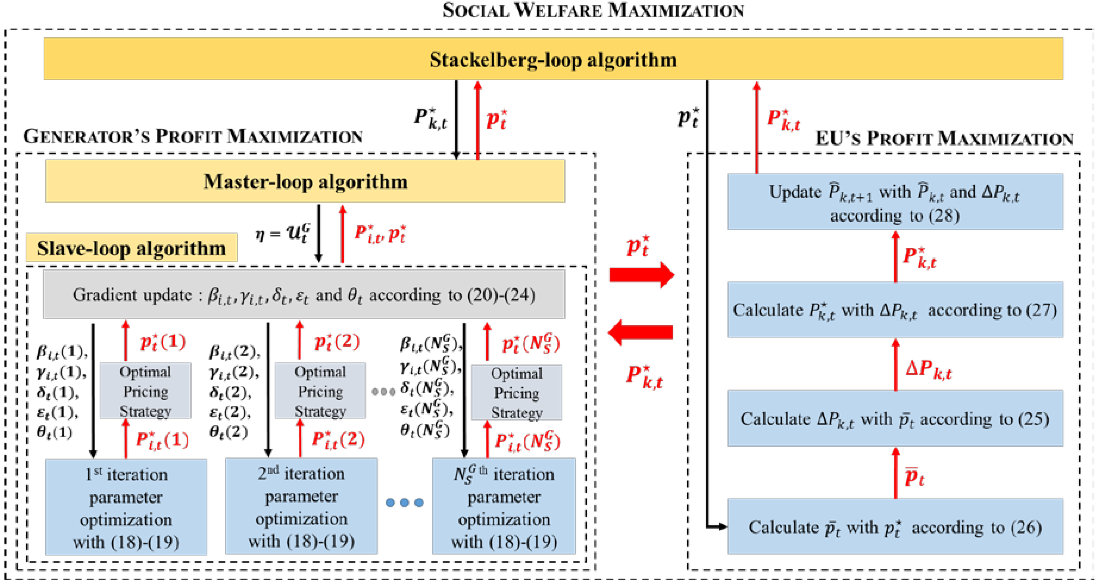
3.4. Schematic Overview and Application of Proposed Algorithms

In this paper, the two game players (generators and EUs) are supposed to participate in the Stackelberg game, and play the game in order to maximize their monetary profit in the smart grid demand response. We proposed two algorithms (Algorithm 1: Generator’s Profit Maximization and Algorithm 2: Energy User’s Profit Maximization) in Section 3.1 and Section 3.2, respectively, as an energy strategy to achieve profit maximization, and the generators and the EUs play Algorithms 1 and 2 alternately in time, respectively, as shown in Figure 2. The proposed game structure is “dynamic game” from the following two reasons:
  • The game players, generators and EUs, interact with observing the each other’s energy strategy for profit maximization. The generators observe the electricity consumption of the EUs, and the EUs observe the electricity price of the generators in the proposed game operation.
  • The proposed profit maximization game was constructed as an iterative algorithm where the energy strategies (Algorithms 1 and 2) are repeatedly performed up to the specified number of times, for example 24 times as 24 h a day.
They play their algorithm in the Stackelberg game and do not play the game at the same time but play alternately over time since the EU needs to know how much the generator has set the current electricity price in order to optimally control his energy consumption P k , t , and the generator needs to know how much power the EU is currently consuming in order to determine the electricity price p t and the amount of power generation in each game play (the game play means the algorithm operation). By running the algorithm repeatedly and alternatively over time and spying on each other’s energy parameters, they can effectively maximize their own profit. The Algorithm for Social-Welfare Maximization is detailed in Algorithms 1 and 2 as the Stackelberg-loop algorithm with the iteration number T . The total architecture of the proposed social welfare maximization including Algorithms 1 and 2 is described in Figure 2 as an overview of the algorithms proposed in this paper.
The proposed methodology to achieve the social-welfare maximization can provide the advantage to maximize the monetary profit of the generators and EUs, but we also reveal the following considering points expected in real-world implementation; 1. Algorithm 1 proposed to maximize the profit of the generator in this paper derives a sub-optimal solution that can reduce the computational complexity compared to the brute-force approach to be suitable for real-time optimization in smart grid demand response. The performance of the algorithm can vary slightly depending on the initial point and the values of the variables that make up the Algorithm; 2. Algorithms 1 and 2 proposed in this manuscript can be implemented in a smart meter or the EMC as a form of software to automatically control the power consumption of energy user’s appliances and facilities. It is a system that can operate only in limited areas equipped with the AMI; 3. Generators are required to have the ability to flexibly control their power generation to participate in the proposed algorithm. We need to consider practical implementations to enable real-time operation of the proposed cooperative and simultaneous usage of coalitional game theory methods.
  • In the EU side, the implementation method of the proposed profit maximization algorithm is as follows: The proposed profit maximization algorithm and formulas is applicable to general demand response applications between generators and EUs such as, residential households, electrical appliances, new smart appliances and internet of things (IoT) devices as a real-world scenario. In the EU side which can be used at high priced hours, we can effectively reduce electricity charges by adjusting the energy usage according to the electricity price with the proposed Market-Adaptive Electricity-Usage Scheduling Algorithm (Algorithm 2 in the manuscript). To implement the Market-Adaptive Electricity-Usage Scheduling Algorithm, automatic electricity usage controller can be needed to be implemented and connected to EU applications (the residential households, IoT devices and etc.). The automatic electricity usage controller can be developed by porting a functional software which quickly and dynamically performs the automatic electricity usage control to an AMI or an EMC. In the case of AMI and EMC, it is possible to transmit and receive electricity price information in real time through power line communications in smart grid. Based on this, the proposed algorithm can be fully implemented and operate to achieve energy usage optimization and electricity charge savings. To summarize, EUs should choose their appliances or facilities to automatically control their energy usage to maximize monetary profit, and if they are connected to a smart meter or EMC equipped with our proposed algorithms, the proposed profit maximization system will simply be able to operate. We think that the proposed system can be implemented in the direction of utilizing existing infrastructure such as the smart meter and EMC.
  • On the generator side, the implementation method of the proposed profit maximization algorithm is as follows: In order to realize the optimal power generation and optimal pricing based on the proposed algorithm in the generators side, the generators should be able to integrate and manage the total power generation and the electricity price by forming a coalitional for profit maximization themselves. Or as a top authority for power generators that are already integrated and managed by the government can implement the proposed coalitional game theory methods. Or a third party such as a power retailer that runs various demand response programs can implement the proposed game theory. If the proposed algorithm is implemented and operated, it should be able to interact with another game player, energy user, with through power line communication or wireless local area network (WLAN) on the smart grid for information communication, such as real-time electricity price and electricity consumption exchange required by this algorithm.
In view of appropriate time intervals for this real-time operation and implementation, we consider the time interval of one hour is reasonable, and we can think about a smaller or larger interval based on this one hour. For example, a 10-min interval that is smaller than 1 h is expected to cause confusion because too much dynamic power generation and power consumption changes for both the generators and the energy users can be caused. On the other hand, if we set a time interval greater than one hour to a time interval, the proposed profit maximization system can be somewhat inefficient if we run the system once a day at a specific time because we have a fairly wide variation in power consumption trends during a day. Therefore, it is reasonable to set the time interval appropriately between minimum 1 h and maximum 24 h in consideration of country, region and environment in which the proposed profit maximization system operates.

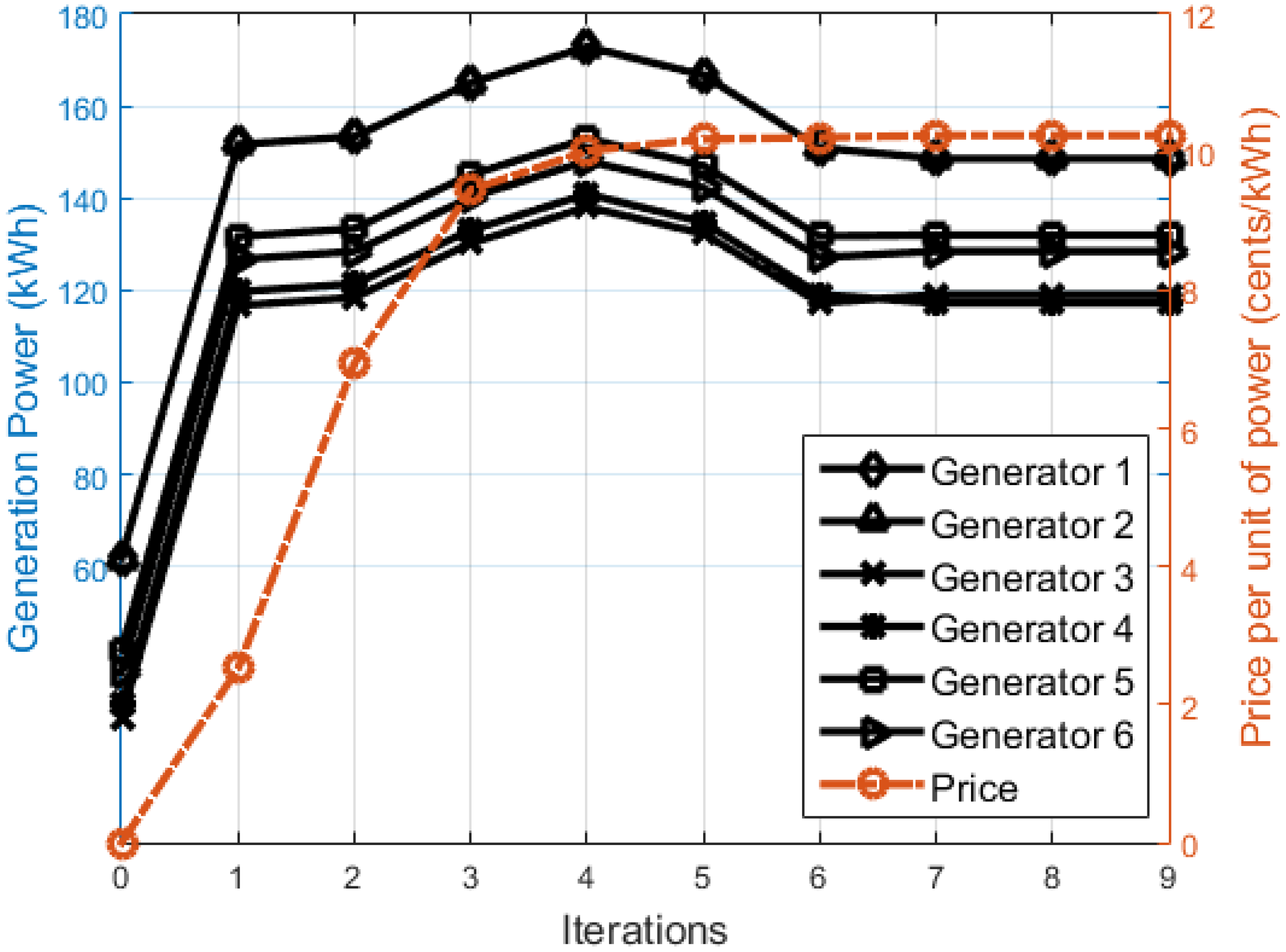
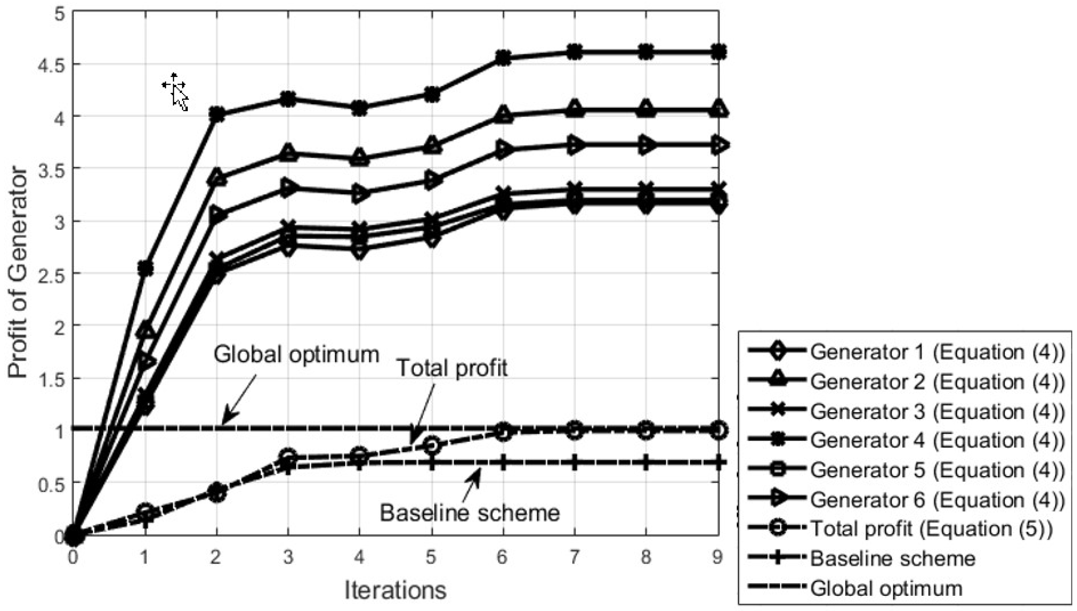
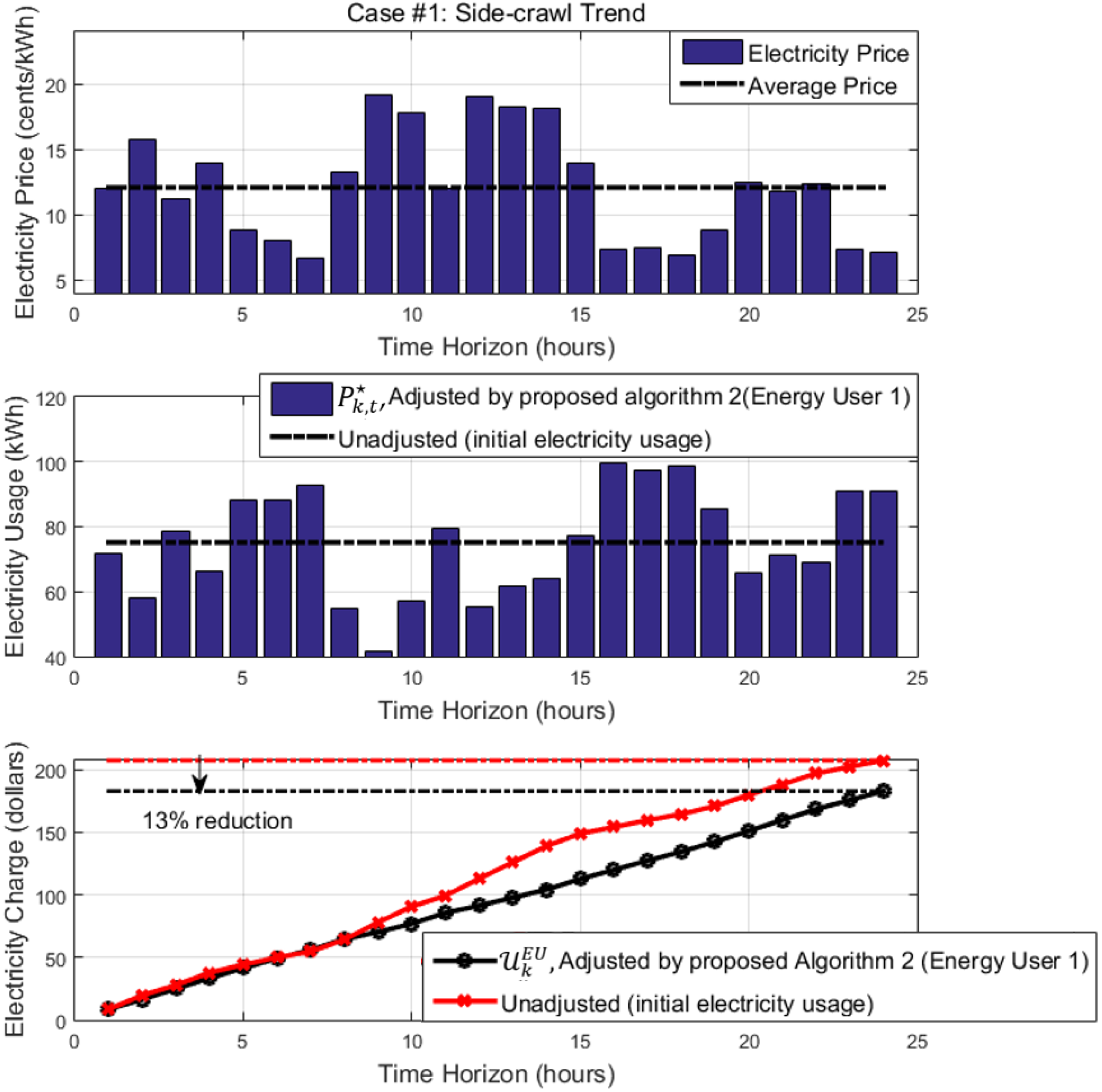
4. Simulation Results

In this section, numerical results are provided to demonstrate the effectiveness of the proposed algorithm. The system setup is as follows: six generators and 12 EUs are considered based on the IEEE 39-BUS system [32]. The graph of the communication network of these generators and EUs shows that they are strongly connected. The parameters of the EUs and the generators are given in Table 2 and Table 3 [32]. The constant time length t l was set to 1 h, and the total scheduling time was set to T = 24 (one day) with the minimum requisite electricity consumption φ k = T ( P k m + P k M ) / 2 . Further, the initial value of the P ^ k , t was set to P ^ k , t = φ k / T , and it was assumed that the lower bound of the electricity price per unit of energy is nonzero, whereas the upper bound is 50 (cents/kWh). The window size t w was set to be from 1 to 10. In the following results, the maximum number of slave-loop iterations was set to 6.
Figure 3 shows the evolution of the generation power (kWh) P i , t and the electricity price (cents/kWh)   p t of each generator optimized by the proposed iterative Algorithm 1. “Iterations” in Figure 3 is the number of master-loop iterations N M G of Algorithm 1, and the result was averaged over 1000 independent simulations, each of which involved different scheduling time slots. From Figure 3, it is evident that the convergence of the generation power and the price can be achieved within seven iterations on average to maximize the U t G . All of the values in each iteration change with satisfying the A G in (9). To maximize the generator profit, the generation power of each generator converges to a different optimal value, which is affected by the constant parameters such as a i , b i , c i , d i , P i m , and P i M , and the price converges to its optimal value in conjunction with the generation power.
Figure 4 demonstrates the evolution of the generator profit calculated with the employment of the optimal values of the generation power and the electricity price from Figure 3. The optimization process is performed using the proposed master- and slave-loop algorithms in Algorithm 1. Even though the generator power curves in Figure 3 show fluctuations with the iterations, it is evident that all of the curves continually increase as the iterations continue. Furthermore, a baseline scheme was set as a profit maximization strategy which optimizes only one of the two optimization parameters ( P i , t , p t ) compared to the proposed Algorithm 1, where the other optimization parameter was fixed. The “fixing” means that the fixed parameter was not optimized but its value is constant, and the fixed value of P i , t was set as just one of the possible values to ( P i m + P i M ) / 2 . In Figure 4, it is confirmed that the profit of the proposed algorithm is greater than that of the baseline scheme, thereby confirming the proper operability of the algorithm. Furthermore, the proposed optimization problem in this paper is a non-convex optimization problem (P1 in Section 2) and the global optimum for the non-convex optimization problem is usually only achieved by using a brute-force approach (or exhaustive search). In this paper, to solve P1, Lagrange dual method and non-linear fractional programming were applied to find a sub-optimal point close to the global optimum. From Figure 4, the global optimum point was further suggested, and it was confirmed that the difference from the sub-optimal point is within 1% when the iteration is converged to 7. Since the sub-optimal point we found may differ depending on the initial point in the proposed profit maximization algorithm. So we propose a method to calculate multiple sub-optimal points with multiple initial points to determine the more maximized point among the multiple sub-optimal points. In the implementation phase, this algorithm should be devised to generate multiple initial points and calculate the sub-optimal point corresponding to the multiple initial points.
Remark 4.
It is not possible to run the baseline scheme by fixing the p t . When the p t is fixed, it is obvious that the P i , t will be set to the minimum value to maximize the profit according to the structure of Equation (4).
In Figure 5, Figure 6 and Figure 7, the electricity price, the electricity usage of one of the EUs according to the price, and the accumulated electricity charge are depicted over time. All of the results were simulated for T = 24 h (one day) with 1-h intervals, and the window size was set to be t w = 3 . Figure 5, Figure 6 and Figure 7 show the changes in the electricity price as Case #1: side-crawl trend, Case #2: rising-tide trend, and Case #3: falling-tide trend, respectively, and these are case studies where the possible trends were analyzed in the real market to determine the effectiveness of the proposed Algorithm 2. Please note that, regarding the totals of Algorithms 1 and 2, Algorithm of Social-Welfare Maximization, the electricity prices of all of these cases were calculated using Algorithm 1, while the electricity usage and the electricity charge were calculated using Algorithm 2. Also, these three cases are three of the results that were obtained by the performance of the entire Algorithm of Social-Welfare Maximization over 1000 times. From Figure 5, Figure 6 and Figure 7, the changes of the electricity usage of EU 1 show that the proposed Algorithm 2 operates in a market-adaptive manner (EU 1 is merely a representative of the EUs, and the rest of the EUs show the same tendency), as the expectation of this is described in Section 3.2. Based on this market-adaptive manner, the electricity usage is reduced when the electricity is expensive, whereas the electricity usage increases when the electricity is cheap, thereby meaning that the total electricity consumption is the same, but the electricity charge can be considerably reduced. Please note that this means that the proposed algorithm can alleviate the existing PAR reduction problem because the electricity usage immediately responds to the price according to the results of Figure 5, Figure 6 and Figure 7. In the real world implementation, it is also possible to alleviate the problem that the price greatly fluctuates because if the price changes greatly, the generators will lose its profits and will not be able to withstand it. We can contribute to stabilization of power generation and PAR reduction, which is one of the ultimate goals of DR through our proposed algorithm. Figure 5, Figure 6 and Figure 7 show that the average electricity usage is the same in any trend according to the A E U , and the electricity charge can be greatly reduced from 13–18%. The comparator, which consumes the same power at all times, is “unadjusted” in the legend. Furthermore, from Figure 5, Figure 6 and Figure 7, it can be seen that the greater the variability in the market, the greater the possibility of the adaptation to the market that facilitates the attainment of a greater benefit.
We can think of the proposed game methodology as a type of DR because the demand is responsive to price as the reviewer commented, but it is not exactly a DR program. In general DR should include the ability to convert excess power consumption to optimal power consumption (“load reduction”), as well as to provide price elasticity to eliminate inefficiencies due to fixed prices. In the proposed game methodology, we do not reduce the power consumption of the energy user, but optimize how efficiently the specified power consumption will be consumed in a given period of time. In Figure 5, Figure 6 and Figure 7, to maximize the profit of the EU, we estimated the adjusted electricity usage which should be consumed for each hour when we know an amount of energy we should use during the day. When the electricity price changes as shown in the top figure of Figure 5, Figure 6 and Figure 7, respectively, the electricity charge can be reduced by 13%, 18% and 16% when calculating the electricity usage as shown in the middle figure of Figure 5, Figure 6 and Figure 7 based on the proposed algorithm. We studied in this paper how to use the load efficiently within the reduced load when the energy user receives an instruction to reduce the load on the DR.
Remark 5.
In the proposed algorithm, the profit function of each generator and EU is defined mathematically in Section 2 so that the profit generation and distribution can be fair. Each generator and EU does not need special skills for fairness because it is an independent entity and can take its own profits by the defined profit function.
Figure 8 represents the way the market volatility (degree of change of the electricity price) provides the EU with benefits when the window size changes from 1 to 10. The benefit function is first given in Figure 8, as follows:
  Benefit = ( 1 U E U   U ¯ E U ) 100
where U ¯ E U is the total electricity charge that is accumulated for the T when the electricity usage is unadjusted and allocated in a totally flat manner. Note that the reduction percentages in Figure 5, Figure 6 and Figure 7 were calculated using Equation (29). Also note that, in Figure 8, the peak-to-average ratio (PAR) is an approximate indicator of the electricity usage as it is known, and it was assumed that the change in the PAR reflects the volatility of the electricity price, because the electricity usage fluctuates when the electricity price fluctuates according to Algorithm 2. It is evident that Algorithm 2 responds sensitively to the changes in the electrical price; that is, the smaller that t w is, the greater the benefit that is derived, with the exception of the case where t w is 1. Here, t w is 1, and this means that the electricity usage has not been adaptively adjusted to the market using Equation (26), while it is also accurate that the PAR is 1. In the meantime, it is possible to observe the trends of the increasing benefit as the PAR is increased, and this means that, as the market volatility is increased, Algorithm 2 can increase the benefit. The purpose of this simulation, however, is not the raising of the PAR to increase the benefit. The purpose is the demonstration of the benefit that is attained from the proposed algorithm when the EU has some PAR.

Summary of Simulation Results and Insights

We showed the results of maximizing the profit of the generators through Algorithm 1 in Figure 3 and Figure 4, and we demonstrated the results of maximizing the profit of the EUs based on Algorithm 2 in Figure 5, Figure 6 and Figure 7. In Figure 3 and Figure 4, we confirmed that the profit of the generators can be improved to about 45% compared to existing (baseline scheme) scheme, and the electricity charge of the EUs can be reduced by 15.6% on average compared to that of when algorithm was not applied. Please note that the amount of power consumption of the EUs is same when the algorithm was applied and not applied. From Figure 3, Figure 4, Figure 5, Figure 6 and Figure 7, we confirmed that the proposed profit maximization algorithms effectively improves the monetary profit of generators and EUs. We summarize the gain of monetary profit from the proposed algorithms in Table 4.
To provide and investigate the influence of the changes of the PAR on the monetary profit generated from the proposed algorithms, Figure 8 showed the change of the profit of the EUs. From Figure 8, we confirmed that the EUs gain more profit as the PAR increases. What this means that more EUs will participate in this game and algorithms when the PAR increases, and it can lead to PAR reduction because the monetary gain that can be obtained for the current PAR has no choice but to be limited, and it can be predicted that as many people share the profit, the PAR would decrease. This also suggest the proposed algorithm not only can contribute to maximization of the profit of the generators and the EUs, but also the desired goal of demand response, PAR reduction, at the same time.

5. Conclusions

In this paper, to maximize the monetary profit in real-time price DR systems, we formulated the Stackelberg game-based non-convex optimization problem, and proposed two energy strategies, Algorithm 1: Generator’s Profit Maximization and Algorithm 2: Energy User’s Profit Maximization, as an optimal solution. In the problem formulation, we newly formulated the generator profit function to reflect the influence of the electricity usage of EUs. To solve the non-convex optimization problem, nonlinear fractional programming and the Lagrange-multiplier method were adopted in proposing the energy strategy for the generators. Also, we newly proposed the energy strategy for the EUs based on the time-window-based market-adaptive manner. We greatly improve the monetary profit of the generators and EUs using the proposed two energy strategies by optimizing the amount of the power generation and the electricity price in the generator side, and electricity consumption in the EU side. In Figure 3 and Figure 4, we confirmed that the profit of the generators can be improved to about 45% compared to the existing (baseline) scheme, and the electricity charge of the EUs can be reduced by 15.6% on average compared to that of when algorithm was not applied. Furthermore, we confirmed that the simulation result from Figure 8 suggests the proposed algorithm can contribute to not only maximization of the profit of the generators and the EUs, but also the desired goal of demand response, PAR reduction, at the same time.

Author Contributions

Y.M.H. has contributed to the theoretical approaches, simulation and preparing the paper; I.S. has contributed to the theoretical approaches and literature review; Y.G.S. has contributed to the theoretical approaches and preparing the paper; H.-J.L. has contributed to the theoretical approaches, literature review and paper writing; J.Y.K. has designed and supervised the paper.

Funding

This work was, in part, supported by Basic Science Research Program through the National Research Foundation of Korea funded by the Ministry of Education (NRF-2016R1D1A1B03933872), and in part supported by “Human Resources Program in Energy Technology (No. 20174010201620)” of the Korea Institute of Energy Technology Evaluation and Planning (KETEP), granted financial resource from the Ministry of Trade, Industry & Energy, Republic of Korea, and in part by Kwangwoon University in 2018.

Conflicts of Interest

The authors declare no conflict of interest.

References

  1. Siano, P. Demand response and smart grids-A survey. Renew. Sustain. Energy Rev. 2014, 30, 461–478. [Google Scholar] [CrossRef]
  2. Wood, A.J.; Wollenberg, B.F. Power Generation, Operation, and Control; John Wiley & Sons: Hoboken, NJ, USA, 2012. [Google Scholar]
  3. Zakariazadeh, A.; Jadid, S.; Siano, P. Smart microgrid energy and reserve scheduling with demand response using stochastic optimization. Int. J. Elect. Power Energy Syst. 2014, 63, 523–533. [Google Scholar] [CrossRef]
  4. Deng, R.; Yang, Z.; Chow, M.-Y.; Chen, J. A survey on demand response in smart grids: Mathematical models and approaches. IEEE Access 2017, 11, 570–582. [Google Scholar] [CrossRef]
  5. Chen, X.; Wei, T.; Hu, S. Uncertainty-aware household appliance scheduling considering dynamic electricity pricing in smart home. IEEE Trans. Smart Grid 2013, 4, 932–941. [Google Scholar] [CrossRef]
  6. Power Smart Pricing. Available online: http://www.powersmartpricing.org/ (accessed on 12 May 2018).
  7. Kim, T.; Poor, H. Scheduling power consumption with price uncertainty. IEEE Trans. Smart Grid 2011, 2, 519–527. [Google Scholar] [CrossRef]
  8. Ibars, C.; Navarro, M.; Giupponi, L. Distributed Demand Management in Smart Grid with a Congestion Game. In Proceedings of the First IEEE International Conference on Smart Grid Communications, Gaithersburg, MD, USA, 4–6 October 2010; pp. 495–500. [Google Scholar] [CrossRef]
  9. Kishore, S.; Snyder, L. An Innovative RTP-based Residential Power Scheduling Scheme for Smart Grids. In Proceedings of the 2011 IEEE International Conference on Acoustics, Speech and Signal Processing (ICASSP), Prague, Czech Republic, 22–27 May 2011; pp. 5956–5959. [Google Scholar] [CrossRef]
  10. Bu, S.; Yu, F.R.; Liu, P.X. Dynamic pricing for demand-side management in the smart grid. In Proceedings of the IEEE Online Conference on Green Communications, New York, NY, USA, 26–29 September 2011; pp. 47–51. [Google Scholar] [CrossRef]
  11. Tavakoli, M.; Shokridehaki, F.; Akorede, M.F.; Marzband, M.; Vechiu, L.; Pouresmaeil, E. CVaR-based energy management scheme for optimal resilience and operational cost in commercial building microgrids. Int. J. Elec. Power Energy Syst. 2018, 100, 1–9. [Google Scholar] [CrossRef]
  12. Tavakoli, M.; Shokridehaki, F.; Marzband, M.; Godina, R.; Pouresmaeil, E. A two stage hierarchical control approach for the optimal energy management in commercial building microgrids based on local wind power and PEVs. Sustain. Cities Soc. 2018, 41, 332–340. [Google Scholar] [CrossRef]
  13. Marzband, M.; Azarinejadian, F.; Savaghebi, M.; Pouresmaeil, E.; Guerrero, J.M.; Lightbody, G. Smart transactive energy framework in grid-connected multiple home microgrids under independent and coalition operations. Renew. Energy 2018, 126, 95–106. [Google Scholar] [CrossRef]
  14. Marzband, M.; Fouladfar, M.H.; Akorede, M.F.; Lightbody, G.; Pouresmaeil, E. Framework for smart transactive energy in home-microgrids considering coalition formation and demand side management. Sustain. Cities Soc. 2018, 40, 136–154. [Google Scholar] [CrossRef]
  15. Tushar, W.; Yuen, C.; Smith, D.B.; Poor, H.V. Price discrimination for energy trading in smart grid: A game theoretic approach. IEEE Trans. Smart Grid 2017, 8, 1790–1801. [Google Scholar] [CrossRef]
  16. Yu, M.; Hong, S.H. A real-time demand-response algorithm for smart grids: A Stackelberg game approach. IEEE Trans. Smart Grid 2016, 7, 879–888. [Google Scholar] [CrossRef]
  17. Ye, M.; Hu, G. Game design and analysis for price-based demand response: An aggregate game approach. IEEE Trans. Cybern. 2017, 47, 720–730. [Google Scholar] [CrossRef] [PubMed]
  18. Hong, S.G.; Hwang, Y.M.; Lee, S.Y.; Shin, Y.; Kim, D.I.; Kim, J.Y. Game-theoretic modeling of backscatter wireless sensor networks under smart interference. IEEE Commun. Lett. 2018, 22, 804–807. [Google Scholar] [CrossRef]
  19. Lee, C.; Park, L.; Cho, S. Light-weight Stackelberg game theoretic demand response scheme for massive smart manufacturing systems. IEEE Access 2018, 6, 23316–23324. [Google Scholar] [CrossRef]
  20. Esfahani, M.M.; Hariri, A.; Mohammed, O.A. A multiagent-based game-theoretic and optimization approach for market operation of multi-microgrid systems. IEEE Trans. Ind. Informat. 2018, 1, 1–12. [Google Scholar] [CrossRef]
  21. Marzband, M.; Javadi, M.; Pourmousavi, S.A.; Lightbody, G. An advance retail electricity market for active distribution systems and home microgrid interoperability based on game theory. Electr. Power Syst. Res. 2018, 157, 187–199. [Google Scholar] [CrossRef]
  22. Nekouei, E.; Alpcan, T.; Chattopadhyay, D. Game-theoretic frameworks for demand response in electricity markets. IEEE Trans. Smart Grid 2015, 6, 748–758. [Google Scholar] [CrossRef]
  23. Asr, N.R.; Ojha, U.; Zhang, Z.; Chow, M.Y. Incremental welfare consensus algorithm for cooperative distributed generation/demand response in smart grid. IEEE Trans. Smart Grid 2014, 5, 2836–2845. [Google Scholar]
  24. Soliman, S.A.-H.; Mantawy, A.-A.H. Modern Optimization Techniques with Applications in Electric Power Systems; Springer: Berlin, Germany, 2011. [Google Scholar]
  25. Zhang, Z.; Chow, M.-Y. Convergence analysis of the incremental cost consensus algorithm under different communication network topologies in a smart grid. IEEE Trans. Power Syst. 2012, 27, 1761–1768. [Google Scholar] [CrossRef]
  26. Yang, S.; Tan, S.; Xu, J.-X. Consensus based approach for economic dispatch problem in a smart grid. IEEE Trans. Power Syst. 2013, 28, 4416–4426. [Google Scholar] [CrossRef]
  27. Kar, S.; Hug, G.; Mohammadi, J.; Moura, J.M.F. Distributed state estimation and energy management in smart grids: A consensus innovations approach. IEEE J. Sel. Top. Signal Process. 2014, 8, 1022–1038. [Google Scholar] [CrossRef]
  28. Liu, Y.; Hu, S.; Huang, H.; Ranjan, R.; Zomaya, A.Y.; Wang, L. Game theoretic market driven smart home scheduling considering energy balancing. IEEE Syst. J. 2017, 11, 910–921. [Google Scholar] [CrossRef]
  29. Dinkelbach, W. On nonlinear fractional programming. Manag. Sci. 1967, 13, 492–498. [Google Scholar] [CrossRef]
  30. Boyed, S.P.; Vandenberghe, L. Convex Optimization; Cambridge University Press: Cambridge, UK, 2004. [Google Scholar]
  31. Azizi, S.; Dobakhshari, A.S.; Sarmadi, S.A.N.; Ranjbar, A.M. Optimal PMU placement by an equivalent linear Formulation for exhaustive search. IEEE Trans. Smart Grid 2012, 3, 174–182. [Google Scholar] [CrossRef]
  32. Ma, K.; Hu, G.; Spanos, C.G. Distributed energy consumption control via real-time pricing feedback in smart grid. IEEE Trans. Control Syst. Technol. 2014, 22, 1907–1914. [Google Scholar] [CrossRef]
Figure 1. Systemic model of social-welfare maximization in a smart grid with demand response (DR) systems.
Energies 11 02315 g001
Figure 2. The diagram of the proposed iterative algorithm for social welfare maximization in smart grid.
Energies 11 02315 g002
Figure 3. Generation power P i , t and electricity price p t versus iteration with I = 6 generators.
Energies 11 02315 g003
Figure 4. Generator profit versus iteration.
Energies 11 02315 g004
Figure 5. Electricity price with time (Case #1: side-crawl trend) and the electricity usage adjusted accordingly, and the confirmation of the electricity-charge saving.
Energies 11 02315 g005
Figure 6. Electricity price with time (Case #2: rising-tide trend) and the electricity usage adjusted accordingly, and the confirmation of the electricity-charge saving.
Energies 11 02315 g006
Figure 7. Electricity price with time (case #3: falling tide trend) and the electricity usage adjusted accordingly and confirmation of electricity charge savings.
Energies 11 02315 g007
Figure 8. Benefits versus window sizes with varying PAR.
Energies 11 02315 g008
Table 1. Notation list.
NotationsMeanings of Notations
K = { 1 , , K } , k K The set of energy users (EUs)
I = { 1 , , I } , i I The set of generators
T = { 1 , , T } , t T Total scheduling time set
t l The constant time length
p t (cents/kWh)The electricity price per unit energy
P i , t (kWh)The amount of the actual providable power
P i , t L (kWh)The transmission losses
P i , t T (kWh)The total amount of generated power
C i , t ( P i , t T ) (cents)The cost to generate power for generator i
a i   ( cents / kWh 2 ) , b i   ( cents / kWh ) , and c i   ( cents ) The fitting parameters of the cost function C i , t ( P i , t T )
d i The coefficient for power loss
P i m and P i M The minimum and maximum bound of P i , t T
U i , t G The profit function for generator i
U t G The total profit for all generators
R t Real profit of generators
M i , t Maximum achievable profit of the generator i
P k , t The amount of the electricity usage of UE k
P ^ k , t The amount of electricity to be used in the future divided by the remaining time
P k , t The additional or abandoned electricity usage
U k E U The electricity charge for UE k
U E U The total electricity charge for all UEs
G = ( N ,   A ,   U ) The Stackelberg game where N is a player set that is composed of generators and EUs, A is the constraint set, and   U is the profit set
p m and p M The minimum and maximum prices of the electricity
P k m and P k M The minimum and maximum electricity-usage
φ k The minimum required electricity consumption
η The optimum solution of P1
P i , t ,   p t and P k , t The optimized value of P i , t , p t and P k , t
F A set of feasible solutions
L G The Lagrange dual function of P3
β i , t , γ i , t , δ t , ε t , and θ t The Lagrange multipliers
N M G and N S G The number of iterations for the master-loop and slave-loop in Algorithm 1
ω 1 , ω 2 , ω 3 , ω 4 , and ω 5 The iteration steps for optimization
p ¯ t The base price as the historical average of p t
t w The window size of the time slots
U ¯ E U The total electricity charge accumulated for T
Table 2. Parameters of generators for IEEE 39-BUS [32].
Generator Parameters
Node   a i     b i     c i     d i     P i m     P i M  
10.00245.56300.0002160339.69
20.00564.32250.0003125479.10
30.00726.60250.0001128290.4
40.00473.14160.0002240306.34
50.00917.5460.0004135593.80
60.00464.76120.00012130443.41
Table 3. Parameters of EUs for IEEE 39-BUS [32].
Demand Parameters
Node   P k m     P k M   Node   P k m     P k M  
150100.34780137.93
2100159.1385084.19
34080.56950104.06
430123.981078119.36
580109.5511103176.19
64076.341267147.26
Table 4. The gain of monetary profit from the proposed algorithm.
Energy StrategyGain of Profit
Algorithm 1: Generator Profit MaximizationAbout 45% (compared to existing (beseline scheme) scheme)
Algorithm 2: Energy User Profit Maximization15.6% on average (compared to that of when algorithm was not applied)

