Lyapunov-Based Large Signal Stability Assessment for VSG Controlled Inverter-Interfaced Distributed Generators

Shanghai Jiao Tong University, Shanghai 200240, China
*
Author to whom correspondence should be addressed.
Energies 2018, 11(9), 2273; https://doi.org/10.3390/en11092273
Submission received: 9 August 2018
/
Revised: 22 August 2018
/
Accepted: 27 August 2018
/
Published: 29 August 2018
(This article belongs to the Special Issue Distribution System Operation and Control)
Abstract
:Inverter-interfaced distributed generators (IIDGs) have been widely applied due to their control flexibility. The stability problems of IIDGs under large signal disturbances, such as large load variations and feeder faults, will cause serious impacts on the system. The virtual synchronous generator (VSG) control is an effective scheme for IIDGs to increase transient stability. However, the existing linearized stability models of IIDGs are limited to small disturbances. Hence, this paper proposes a Lyapunov approach based on non-linearized models to assess the large signal stability of VSG-IIDG. The electrostatic machine model is introduced to establish the equivalent nonlinear model. On the basis of Popov’s theory, a Lyapunov function is derived to calculate the transient stability domain. The stability mechanism is revealed by depicting the stability domain using the locus of the angle and the angular frequency. Large signal stability of the VSG-IIDG is quantified according to the boundary of the stability domain. Effects and sensitivity analysis of the key parameters including the cable impedance, the load power, and the virtual inertia on the stability of the VSG-IIDG are also presented. The simulations are performed in PSCAD/EMTDC and the results demonstrate the proposed large signal stability assessment method.
1. Introduction
Inverter-interfaced distributed generators (IIDGs) feature in flexible control and quick response uses in different application scenarios. However, unlike conventional synchronous generators, inverters lack inertia [1]. High penetration of IIDGs may result in poor voltage and frequency response, and even instability with large-scale oscillation, asynchronism, and voltage collapse under large disturbances [2]. The virtual synchronous generator (VSG) control scheme is an effective solution to the assigned problem. By controlling the switching pattern of the inverter, the VSG emulates conventional synchronous generators. The VSG means to provide virtual inertia and additional damping that can reduce frequency deviations during disturbances [3,4]. The VSG controlled IIDG (VSG-IIDG) is becoming one of the most prospective renewable sources due to the outstanding features [5].
The stability issues of VSG-IIDGs are categorized into two types: small signal stability and large signal stability. Small signal stability of IIDG has been relatively perfected using the concept of synchronous generators in references [6,7]. The study of small signal stability uses the linearized model. Nyquist or Routh-Hurwitz stability criterion, eigenvalue analysis [8,9,10,11], and transfer function [12,13] are the regular tools to assess the small signal stability. However, the analysis of the small signal linearized model is only valid around the stable operating point yet not accurate under large disturbances. The behavior of VSG-IIDGs under large disturbances should be explored with nonlinear models of large signal stability. Large signal nonlinear analysis has wider application range and higher reliability. Besides, the stability domain can be obtained via the study of large signal stability. A large signal stable system is small signal stable yet the opposite is not true [14].
There are few studies presently on the large signal stability of VSG-IIDG due to various nonlinear factors [14]. Lyapunov-based methods are commonly used in the analysis of large signal stability. The main advantage of the methods is that they have a distinct computational performance. The stability assessment using Lyapunov theory is based on comparing the transient energy at fault clearing time with the critical energy without developing numerical computer models of the system [15]. Control models based on Lyapunov theory were proposed in references [16,17] for the integration of distributed generators into the distribution network. A Lyapunov function was established in [18] to prove the convergence of the proposed VSG control strategy. However, the transient stability mechanism and performance of VSG-IIDGs under large signal disturbances were not provided. Reference [19] investigated how transient energy of VSG-IIDG would be stored and released during disturbances using a Lyapunov function. Nevertheless, these studies address little on the assessment of large signal stability. The stability domain has not been depicted clearly. A valid Lyapunov function should be established to determine the stability domain. The mechanism of large signal stability, as well as the effect of parameters on the stability domain, needs to be further explored. Besides, further research is needed to establish the mathematical model of the VSG-IIDG for large signal nonlinear study. Reference [20] adopted the electrostatic machine model to establish the equivalent circuit of the droop-controlled IIDG. The Lyapunov function in [20] was not applicable to the stability assessment of the VSG-IIDG, but it provided reference values for the large signal stability study of the VSG-IIDG.
This paper focuses on large signal stability assessment of the VSG-IIDG. The contributions of the paper are threefold: (1) A nonlinear mathematical model of the VSG-IIDG is established by applying the equivalent model of an electrostatic machine. This nonlinear model combining both the electrical parts and control signals can be an analytical tool for the study of large signal stability (2). Based on Popov’s theory, a Lyapunov function is derived and the stability domain of IIDG is determined. This Lyapunov-based method has a distinct computational advantage. The stability assessment is based on comparing the transient energy of the postfault system with the critical energy without developing numerical computer models of the system (3). The large signal stability mechanism of VSG-IIDGs is revealed by analyzing the boundary of the stability domain. The boundary of the stability domain quantifies the magnitude of the deviation that the system can tolerate. The area of the stability domain reflects large signal stability in an intuitive way. The effect and sensitivity analysis of parameters on the stability domain are presented. The contributing factors of large signal stability are analyzed.
The sections of the paper are organized as follows: Section 2 analyzes the typical VSG control scheme of IIDG and establishes the equivalent electrostatic machine model. The nonlinear state matrix of the VSG-IIDG system is derived in Section 3. In Section 4, a Lyapunov function and the critical stability energy are figured out. The stability domain is defined accordingly. Simulation is conducted in Section 5 and the effect of parameters on the stability domain is analyzed.
2. Typical VSG Control Scheme and Its Equivalent Model for IIDG
2.1. The VSG Control Scheme of IIDG
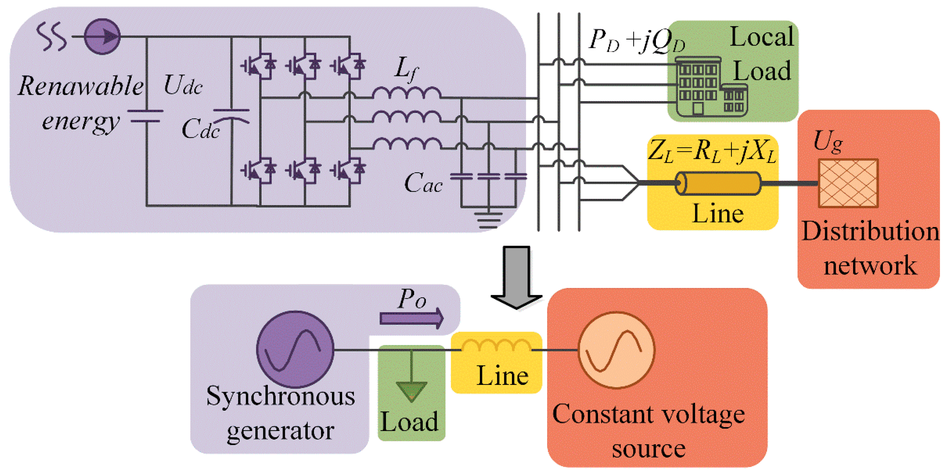
The control scheme of the VSG-IIDG is shown in Figure 1. By controlling the switching pattern of the inverter, the VSG-IIDG has the dynamic properties of the synchronous generator (Figure 2). Given the fact that the capacity of the IIDG is much smaller than that of the host grid, the point of common coupling of VSG-IIDG is equivalent to an infinite bus (similar to single-machine-infinite-bus power system) and is regarded as a constant voltage source. In order to stress the key findings, the fluctuation of the renewable energy is ignored and the voltage at the DC-link capacitance is supposed to be constant. Besides, in order to simplify the analysis, the local load is represented by resistors and inductances.
For conventional synchronous generators, the inertia and damping play a significant role in terms of stability. However, the inner angle frequency of IIDGs is determined by the control scheme. The P-ω controller implements frequency adjustment in the VSG control [21]. The control function of the P-ω controller is expressed as Equation (1):
The P-ω controller imitates the behavior of a conventional synchronous generator and keeps the VSG-IIDG track the frequency of the host network.
2.2. VSG-IIDG Equivalent Electrostatic Machine Model
The stability assessment for VSG-IIDG depends on the nonlinear models. Andrade proposed the idea of modeling the inverter as an electrostatic machine [22]. The concept of electrostatic machine establishes a direct relationship between the DC and AC side of the inverter. This model allows the further introduction of traditional Lyapunov function and facilitates the analysis.
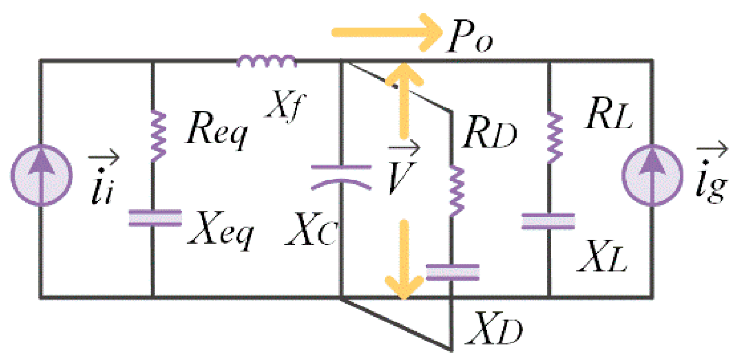
As shown in Figure 3, the IIDG is modeled as an electrostatic machine which is supplied by the direct voltage Udc. The electrostatic machine produces an electric field that induces alternating charges in the armature circuit. “Self” and “mutual” capacitances are included. The rotating reference frame (DQ0) is applied to link dc-side and ac-side. The electric field magnitude and the speed of the rotation parameters are related with Udc and the synthesized voltage reference vector . Briefly, the changes in VSG-IIDG are represented by the changes in charges. Further derivation in [22] takes IIDG as a current source with equivalent resistance and admittance relevant to parameters of the inverter:
We substitute this electrostatic machine model into the IIDG system. The equivalent circuit of the IIDG system is shown in Figure 4. This equivalent circuit combines both the electrical part and control signals. It is used as the model for further study on large signal stability.
3. The Nonlinear Mathematical Model of VSG-IIDG
The equivalent circuit of IIDG system can be described as follows, by using Equation (1):
where, , and are related to the parameters of the equivalent circuit in Figure 4. The specific expression is presented in the Appendix A. Equation (3) can be seen as the expression of Figure 4 in mathematical form. Integrating the electrical parts with control signals, Equation (3) offers a mathematical model for stability study.
Next, the equilibrium point is calculated from (5) when the system runs in a zero-deviation state:
The state equation is normally based on equilibrium points so as to characterize the motion state of the system and facilitate the analysis of deviation. Define state variable x:
Then the mathematical model of the IIDG system is transferred from the equilibrium point to origin point. Hence the state equation in matrix formulation is:
where, , , .
Equation (6) is the expression describing the relationship between the input and the state of the IIDG system. The order of state matrix A is one, hence, matrix A is a singular matrix. It has two characteristic roots. One is zero and the other is . The control parameter H and k are greater than zero, so is in the open left half-plane. In order to facilitate the analysis, Equation (6) can be transformed into the following form through a non-singular transformation by reducing the order of x:
where, .
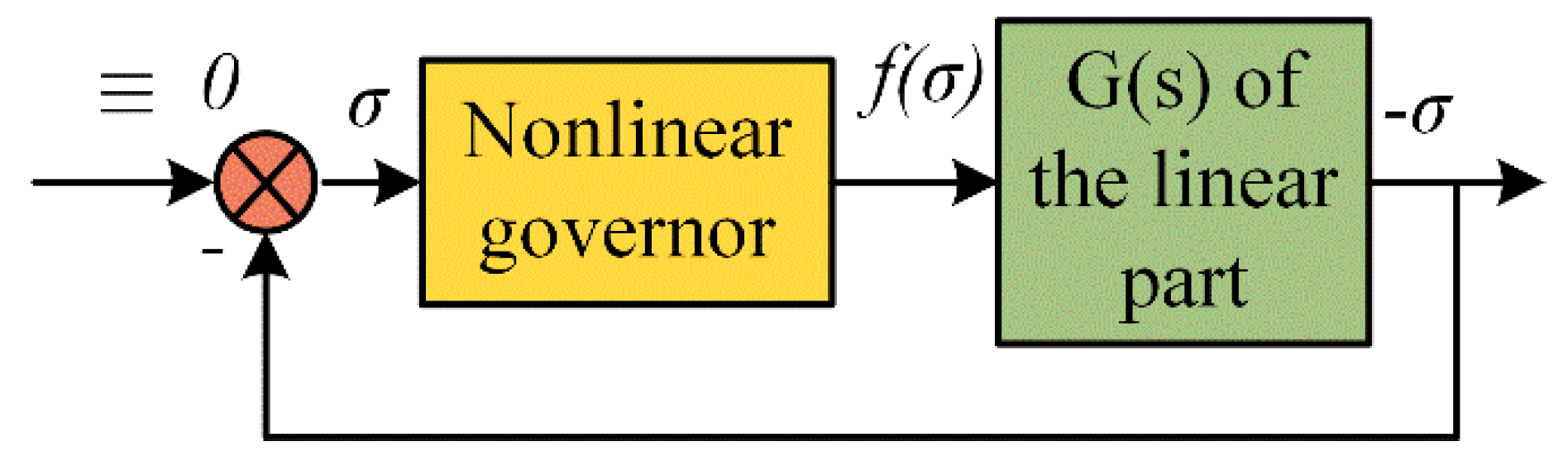
The VSG-IIDG can be seen as a nonlinear system shown in Figure 5 where the control signals are tuned through both the nonlinear governor and the linear governor. The nonlinear part corresponds to the nonlinear function in Equation (6).
In terms of the linear part, the transfer function is obtained as in Equation (8). The nonlinear function and the transfer function are both important in the study of large signal stability.
4. Lyapunov Function Construction and the Stability Domain Determination
In the following sections, the direct method of Lyapunov is applied to study the large signal stability of the VSG-IIDG. The approach uses a Lyapunov function V(x) to estimate the stability domain of the postfault system. The precondition is that this Lyapunov function satisfies the Popov’s theory on stability. The stability domain is defined by an inequality of V(x) < M, where M is a constant representing the critical stability energy. This method quantifies the extent of the deviation that the system can tolerate and features a remarkable computational advantage by simply comparing V with the critical energy rather than conventional step-by-step methods [15].
4.1. Popov stability Criterion
According to Popov’s Theory, in the system as (7), there exists a finite region of asymptotic stability if a real number exists that:
for all ω > 0.
Figure 6 shows a graph drawing on the complex plane. The crux of the Popov condition is to find a straight line of slope 1/q passing through the origin such that the imaginary part of lies categorically under it with points of tangency permitted. In Figure 6, , , and satisfy the Popov condition, whereas and do not. There can be many straight lines meeting the condition (the lines between and ) and the figure only shows four of them. The different choices of the straight line, or to be exact, the values of q are related to the conservativeness of the stability analysis.
Apply the Popov condition to the system whose state equation is shown as (6):
The inequality holds when , and we choose as indicated in [23]. Then we can use the q as a parameter to construct a Lyapunov function.
4.2. Lyapunov Function
This paper applies Kalman’s algorithm [24] to construct the Lyapunov function. The algorithm uses the q as a parameter. Kalman has proved that the Lyapunov function is positive definite with the semi-negative definite derivative. The Lyapunov function so derived satisfies the Popov condition.
- (a)
- Define the function as:where:
- (b)
- Factorize as: . Hence is:
- (c)
- Define the leading coefficient of the polynomial in ascending powers when in a . Then define a vector u with its components being the coefficients of the polynomial in ascending powers. Here the vector u reduces to a scalar in the VSG-IIDG model:
- (d)
- Figure out the symmetric positive definite matrix by solving the Lyapunov matrix equation:Here the Lyapunov matrix equation reduces to the scalar equation so that:
- (e)
- Get the Lyapunov function:
To be more intuitive and convenient, the Lyapunov function needs to be transformed in terms of x. Hence the Lyapunov function of the VSG-IIDG is as follows:
4.3. Lyapunov-Based Large Signal Stability Domain
The stability domain is defined by an inequality of form V(x) < M, where M is a constant representing the critical stability energy. With a Lyapunov function like (18), reference [25] uses Lagrange multipliers to define the critical stability energy M. Hence, the critical stability energy M of stability region is as Equation (19) in the system (6):
The inequality to find stability domain can be expressed as:
Inequality (20) gives an effective way of determining the stability domain. If the operating points of postfault system satisfy inequality (20), it indicates that the VSG-IIDG is large-signal stable. The VSG-IIDG system can recuperate and return to the equilibrium stability where . The complexity of the stability issue of VSG-IIDGs lies in two aspects. First, the VSG control is realized by power electronic devices, hence the features of inverters should be considered. Besides, the VSG emulates the behavior of a synchronous generator. The stability problems similar to conventional synchronous generators will definitely be involved [26]. Inequality (20) takes both of them into consideration. The impact of control parameters has been reflected in the coefficients. The stability domain can be depicted by solving the equation .
Table 1 presents the steps of determining whether a postfault IIDG system is large signal stable based on stability domain. First, the electrical and control parameters is given to establish the IIDG model. Then, the output power is obtained as Equation (27) and the equilibrium point is figured out according to Equation (4). The equilibrium point is used to derive the state equation and obtain b and c in Equation (6). Therefore, the Lyapunov function can be established as Equation (18), and the critical stability energy M of the stability region is calculated according to Equation (19). Then compare the value of the Lyapunov function with the critical M. Smaller function value indicates that the IIDG system is large signal stable.
5. Study Cases
5.1. Parameters of the Simulation Case
Simulations are performed in PSCAD/EMTDC to evaluate the large signal stability of the VSG-IIDG system. The topology and control scheme of the VSG-IIDG system is shown in Figure 1 and Figure 2. Parameters of the VSG-IIDG and the interconnected network are listed in Table 2. A solid three-phase line-to-ground fault of happens in the middle of the transmission line at 3 s.
According to Equation (4), the equilibrium point of VSG-IIDG is:
Substitute the above data for Equation (6), and the state equation of the IIDG system yields as:
5.2. Large Signal Stability Analysis of the VSG-IIDG
The metallic short-circuit fault happens in the middle of the cable at the time of 3 s and is cleared after variable time delays. Once the fault is cleared, and deviate from the equilibrium point at various degrees (different values of and ). It means operating points with different values of the Lyapunov function .
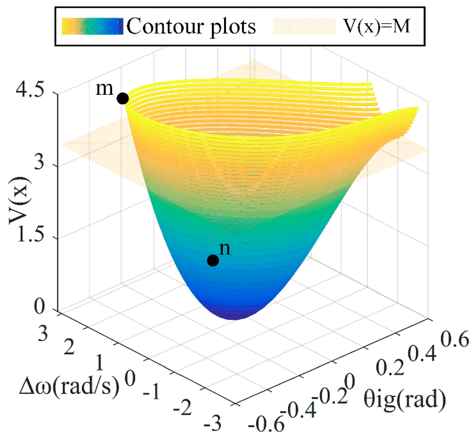
Figure 7 shows the contour plots of the Lyapunov function of operating points with different and . Deviating from the equilibrium point at various degrees, the values of the Lyapunov function are diverse. For the points inside the stability domain, the value of the Lyapunov function is under the critical value M, which indicates that the system is asymptotic stability when operated in these points. Figure 8 shows that the stability domain is in a conical type. Whichever disturbance that has angular frequency and angle limited in the taper can recuperate the system.
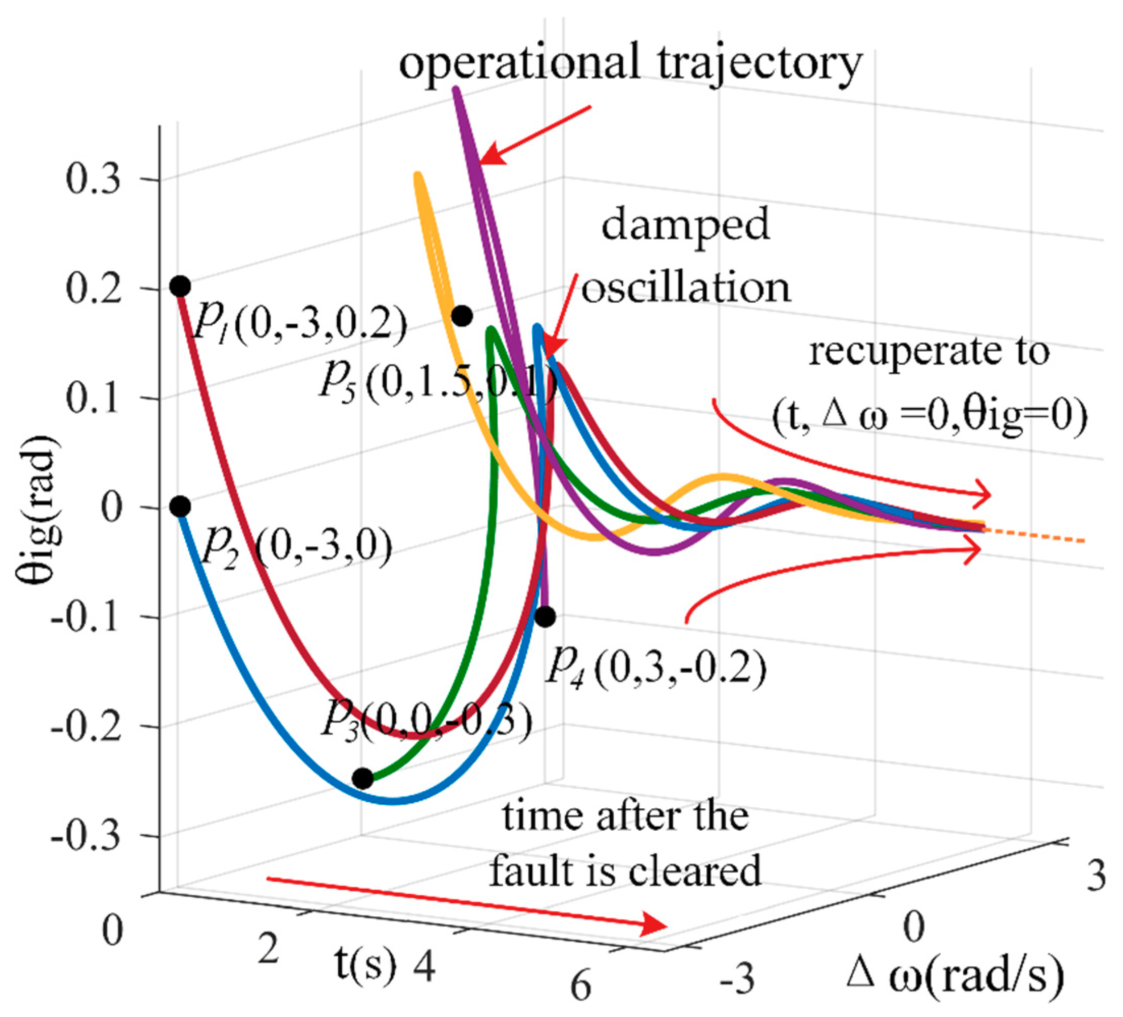
Figure 8 shows the operational trajectories of five stable points (p1–p5) whose Lyapunov function value is less than the critical value M. The abscissa axis of time starts after the fault is cleared. These curves display the deviation of angular frequency and angle from a disturbance condition. It can be observed that after the fault is cleared, these operational trajectories tend to the equilibrium points where . Even though these operational trajectories deviate from the equilibrium point at various degrees, as time pass by, the system finally runs in a zero-deviation state.
When it comes to the unstable operating points, it is quite different. Take an unstable point m and a stable operating point n as example. The point m comes when the fault is cleared at 3.15 s and the deviation , . While the point n comes when the fault is cleared at 3.1 s and the deviation , . As shown in Figure 7, the Lyapunov function values of point m and n are on the different sides of the contour plane of the critical stability energy M. The Lyapunov function value of point n is smaller than the critical stability energy M, which indicated it is inside the stability domain. However, the Lyapunov function value of point m is greater than the critical stability energy M and it is an unstable point.
Figure 9 shows the comparison of simulations of the unstable point m and the stable operating point n. Due to different fault clearing time of these two points, the extent of disturbance varies (different values of and ). As Figure 9a shows, the operational trajectory of the stable point n experiences damped oscillations before reaching the equilibrium stability where . The angular frequency gets slowly back to the reference value and the angle difference between the VSG-IIDG and the network reduces to zero. However, the trajectory of the unstable point m is divergent and of extreme volatility. Even when the fault is cleared, the angular frequency can’t keep in synchronism. The system can’t recuperate and tends to instability. The simulations shown in Figure 9 verify the analysis results.
5.3. The Impact of Parameters on the Stability Domain
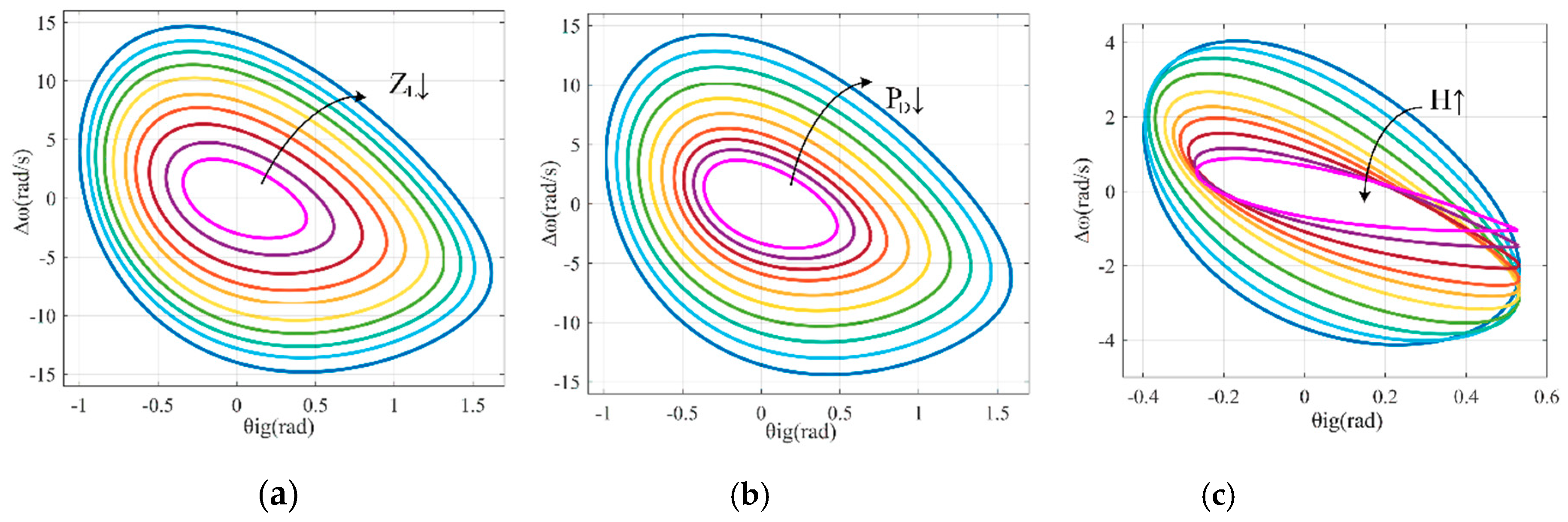
The cable impedance, load power, and virtual inertia have a significant influence on the stability of VSG-IIDG [27,28]. The stability domain with different parameters will be explained in the next sections. The stability domain is determined by the boundary of the equation V(x) = M. The boundary quantifies the extent of disturbances that the VSG-IIDG system can endure. In the simulation, only one parameter is changed and the others are kept the same in different scenarios.
Figure 10a depicts the impact of the impedance of cable () on the stability domain. As impedance decreases, the stability domain expands in the ratio of equality. The increase in impedance means the connection between the IIDG and the network is less. When the supporting function of the network is weakened, the IIDG system is apt to instability.
Figure 10b shows the change of the stability domain when load power decreases. When load power decreases, the stability domain tends to increase. This is due to the fact that a larger load power adds more burden to the system. This is similar to the power angle stability of conventional synchronous generators, where lower power causes relative increase of the acceleration area and out-of-step situations will be rare.
The effect of different virtual inertia H on the stability domain is shown in Figure 10c. As the virtual inertia increases, the stability domain is prone to be smaller. What’s more, the shrink doesn’t happen in the ratio of equality. The shape of boundary changes and a peak appears.
Figure 10c shows that the rising virtual inertia has a negative effect on the large signal stability of the VSG-IIDG. In large signal stability of conventional synchronous generators, the change of inertia does not contribute to the change of the stability boundary [29]. However, it’s not the case in the VSG algorithm and Figure 10c witnesses a marked distortion of the stability domain as virtual inertia increases.
It should be noted that the rising virtual inertia will also slow down the response speed of the IIDG system since it can be seen as an integration constant. Hence the rising virtual inertia leads to a decrease not only in the distance between an operating point and the stability boundary but also the speed running from this point to the boundary. When the distance and speed are reduced simultaneously, it’s not sure whether the time duration will be shortened or not. That means, the critical cleaning time of the fault may not decrease even with a large virtual inertia (a smaller stability domain), since the response speed of the IIDG system is slow and there is still enough time to diagnose and handle the fault.
Table 3 presents the stability of the VSG-IIDG with different values of load power, cable impedance, and virtual inertia when the clearing time is 0.1 s. As shown in the table, when active power of local load increases, the IIDG system tends to instability. When load power and control parameter H remain unchanged, the IIDG system is unstable with larger cable impedance. Also, when the inertia is too large, the stability of the system goes from stable to unstable. The results show in Table 3 indicate that the IIDG system is apt to be unstable with larger load power and cable impedance or smaller virtual inertia.
5.4. Sensitivity Analysis of Parameters
Investigation of the large signal stability by ad hoc variations of the parameters is challenging, especially when several parameters act at the same time. Sensitivity analysis is helpful in identify which parameter should be modified in an easier way. Such studies are of high importance, considering the assessment of large signal stability in different scenarios with large expected variations in grid configurations, operating conditions, and system parameters.
This paper draws on the experience of transient stability analysis in conventional power system [30]. The sensitivity analysis of the load power, cable impedance, and virtual inertia on the stability domain area is performed. The definition of the sensitivity is in partial differential equation as:
where, is the area of stability domain, y is the parameter to be analyzed (load power , cable impedance , and virtual inertia H). The results are shown in Table 4, respectively.
It can be seen that the stability domain is mainly sensitive to load power, cable impedance, and virtual inertia. The sensitivity does not change a lot when different values of load power and cable impedance are adopted. When virtual inertia is kept at a small value, the area of stability domain changes slowly as inertia varies. It should be pointed out that only the virtual inertia can be modified to improve the stability of a control strategy. The load power and cable impedance cannot be influenced by the control. However, the load power and cable impedance can be selected within the proper range during the design of the system.
6. Conclusions
This paper assesses the large signal stability of the VSG-IIDG and derives the boundary of the stability domain:
- (1)
- The nonlinear mathematical model of the VSG-IIDG is established. The equivalent model of electrostatic machine is applied. Both the electrical parts and control signals are taken into account. This nonlinear model can be an analytical tool for the study of large signal stability.
- (2)
- A Lyapunov function is derived based on Popov’s theory to determine the stability of IIDG. By comparing the transient energy of the post-fault system with the critical energy, this Lyapunov-based method has a distinct computational advantage.
- (3)
- The stability domain is depicted and the large signal stability mechanism of VSG-IIDGs is revealed. The stability domain quantifies the magnitude of the deviation that the system can tolerate. The impacts and sensitivity analysis of parameters on the stability domain are presented. The results indicate that large disturbances may lead to instability of the VSG-IIDG with deviation and oscillation of angular frequency. The VSG-IIDG tends to instability with larger load power and cable impedance or smaller virtual inertia.
The study contributes to the further studies of large signal stability. The results have great significance for the design, operation, and planning of the VSG control scheme. What’s more, the analysis of transient process and mechanism of the VSG is helpful in further research on protection and fault analysis.
Author Contributions
Writing—original draft, data curation, formal analysis, M.L.; project administration, methodology, writing—review & editing, W.H.; writing—review & editing, validation, M.Y.; resources, supervision, N.T.
Funding
This research was funded by [National Key Research and Development Program of China] grant number [2017YFB0903202], [Shanghai Sailing Program] grant number [17YF1410200], [National Natural Science Foundation of China] grant number [51807117].
Conflicts of Interest
The authors declare no conflicts of interest.
Nomenclature
| the power angle of the IIDG | |
| the power angle difference between and | |
| the equilibrium point | |
| the power angle of the common coupling point of VSG-IIDG | |
| ω | virtual angular frequency |
| angular frequency reference | |
| the angular frequency difference between ω and | |
| ,, | filtering capacitance of VSG-IIDG and the relative reactance and admittance |
| capacitance of the DC link of VSG-IIDG | |
| H | virtual inertia of the VSG-IIDG |
| ,,,, | inductor, resistance, reactance, admittance, and impedance of the cable |
| ,, | filtering inductor of VSG-IIDG and the relative reactance and admittance |
| M | critical stability energy |
| ,,,, | active power, reactive power, equivalent resistance, reactance, and admittance of the local load |
| Po | output active power measurement of the IIDG |
| active power reference of the IIDG | |
| ,, | the equivalent resistance, reactance, and admittance of the equivalent IIDG current source |
| the area of stability domain | |
| voltage at the DC link of VSG-IIDG | |
| voltage at the point of common coupling | |
| , | average values of voltage modulation for the duty cycle in d and q axis |
| the synthesized voltage reference vector in VSG control | |
| k | the damping factor of VSG-IIDG |
| the sensitivity | |
| q | Popov coefficient |
Appendix A
In Figure 4, and are the equivalent current source of the IIDG and the DN. is the difference of the angle:
and are the admittances of LC filter. is the admittance of transmission line. and are the equivalent admittance of load and IIDG. The expressions are:
The output voltage of IIDG V can be expressed as:
where: .
Hence, the output power of the VSG-IIDG in Figure 5 can be expressed as:
where: .
References
- Shuai, Z.; Sun, Y.; Shen, Z.J.; Tian, W. Microgrid stability: Classification and a review. Renew. Sustain. Energy Rev. 2016, 58, 167–179. [Google Scholar] [CrossRef]
- Soni, N.; Doolla, S.; Chandorkar, M.C. Improvement of Transient Response in Microgrids Using Virtual Inertia. IEEE Trans. Power Deliv. 2013, 28, 1830–1838. [Google Scholar] [CrossRef]
- Liu, J.; Miura, Y.; Bevrani, H. Enhanced Virtual Synchronous Generator Control for Parallel Inverters in Microgrids. IEEE Trans. Smart Grid 2017, 8, 2268–2277. [Google Scholar] [CrossRef]
- Chen, L.; Wang, R.; Zheng, T. Optimal Control of Transient Response of Virtual Synchronous Generator Based on Adaptive Parameter Adjustment. Proc. CSEE 2016, 11, 5724–5731. [Google Scholar]
- Zhang, X.; Zhu, D.; Xu, H. Review of Virtual Synchronous Generator Technology in Distributed Generation. J. Power Supply 2012, 10, 1–6. [Google Scholar]
- Mehrasa, M.; Godina, R.; Pouresmaeil, E.; Vechiu, I.; Rodríguez, R.L.; Catalão, J.P. Synchronous active proportional resonant-based control technique for high penetration of distributed generation units into power grids. Presented at the IEEE Pes Innovative Smart Grid Technologies Conference Europe, Torino, Italy, 26–29 September 2017; pp. 1–6. [Google Scholar]
- Pouresmaeil, E.; Mehrasa, M.; Godina, R. Double synchronous controller for integration of large-scale renewable energy sources into a low-inertia power grid. Presented at the IEEE Pes Innovative Smart Grid Technologies Conference Europe, Torino, Italy, 26–29 September 2017; pp. 1–6. [Google Scholar]
- D’Arco, S.; Suul, J.A.; Fosso, O.B. A virtual synchronous machine implementation for distributed control of power converters in Smart Grids. Electr. Power Syst. Res. 2015, 122, 180–197. [Google Scholar] [CrossRef]
- Meng, J.; Wang, Y.; Shi, X. Control strategy and parameter analysis of distributed inverter based on virtual synchronous generator. Trans. China Electrotech. Soc. 2014, 29, 1–10. [Google Scholar]
- Du, Y.; Su, J.; Zhang, Z. A mode adaptive FM control method for microgrid. China J. Electr. Eng. 2013, 33, 67–75. [Google Scholar]
- Mehrasa, M.; Pouresmaeil, E.; Zabihi, S.; Vechiu, I.; Catalão, J.P. A multi-loop control technique for the stable operation of modular multilevel converters in HVDC transmission systems. Int. J. Electr. Power Energy Syst. 2018, 96, 194–207. [Google Scholar] [CrossRef]
- Cheng, C.; Yang, H.; Zeng, Z. Adaptive control method of rotor inertia for virtual synchronous generator. Autom. Electr. Power Syst. 2015, 19, 82–89. [Google Scholar]
- Huang, L.; Xin, H.; Huang, W. Quantitative analysis method of frequency response characteristics of power system with virtual inertia. Autom. Electr. Power Syst. 2018, 42, 31–38. [Google Scholar]
- Zhu, S.; Liu, K.; Qin, L. A review of transient stability analysis for power electronic systems. Proc. Chin. Acad. Electr. Eng. 2017, 37, 3948–3962. [Google Scholar]
- Kabalan, M.; Singh, P.; Niebur, D. Large Signal Lyapunov-Based Stability Studies in Microgrids: A Review. IEEE Trans. Smart Grid 2017, 8, 2287–2295. [Google Scholar] [CrossRef]
- Mehrasa, M.; Adabi, M.E.; Pouresmaeil, E. Direct Lyapunov control (DLC) technique for distributed generation (DG) technology. Electr. Eng. 2014, 96, 309–321. [Google Scholar] [CrossRef]
- Mehrasa, M.; Pouresmaeil, E.; Catalao, J.P.S. Direct Lyapunov Control Technique for the Stable Operation of Multilevel Converter-Based Distributed Generation in Power Grid. Emerg. Sel. Top. Power Electr. 2014, 2, 931–941. [Google Scholar] [CrossRef]
- Liu, Y.; Chen, J.; Hou, X. Dynamic frequency stabilization control strategy for microgrid based on the adaptive virtual inertial system. Autom. Electr. Power Syst. 2018, 42, 75–82. [Google Scholar] [CrossRef]
- Alipoor, J.; Miura, Y.; Ise, T. Power system stabilization using a virtual synchronous generator with alternating moment of inertia. IEEE J. Emerg. Sel. Top. Power Electr. 2015, 3, 451–458. [Google Scholar] [CrossRef]
- Andrade, F.; Kampouropoulos, K.; Romeral Martínez, J.L.; Vasquez Quintero, J.C.; Guerrero, J.M. Study of large-signal stability of an inverter-based generator using a Lyapunov function. Presented at the 40th Annual Conference of the IEEE Industrial Electronics Society, Dallas, TX, USA, 29 October–1 November 2014; pp. 1840–1846. [Google Scholar]
- Gao, F.; Iravani, M.R. A Control Strategy for a Distributed Generation Unit in Grid-Connected and Autonomous Modes of Operation. IEEE Trans. Power Deliv. 2008, 23, 850–859. [Google Scholar]
- Andrade, F.A.; Romeral, L.; Cusido, J. New model of a converter-based generator using electrostatic synchronous machine concept. IEEE Trans. Energy Convers. 2014, 29, 344–353. [Google Scholar]
- Pai, M.A.; Mohan, M.A.; Rao, J.G. Power System Transient Stability: Regions Using Popov’s Method. IEEE Trans. Power Appl. Syst. 1970, PAS-89, 788–794. [Google Scholar] [CrossRef]
- Kalman, R.E. Liapunov functions for the problem of Lur’e solving (8b): In automatic control. Proc. Natl. Acad. Sci. USA 1963, 49, 201–205. [Google Scholar] [CrossRef] [PubMed]
- Walker, J.A.; McClamroch, N.H. Finite regions of attraction for problem of Lur’e. Intern. J. Control 1967, 6, 331–336. [Google Scholar] [CrossRef]
- Wang, X.; Jiang, H.; Liu, H. Summary of the research on virtual synchronous generator grid connection stability. North China Power Technol. 2017, 9, 14–21. [Google Scholar]
- Renedo, J.; GarcíA-Cerrada, A.; Rouco, L. Active power control strategies for transient stability enhancement of AC/DC grids with VSC-HVDC multi-terminal systems. IEEE Trans. Power Syst. 2016, 31, 4595–4604. [Google Scholar] [CrossRef]
- Hu, T. A nonlinear-system approach to analysis and design of power-electronic converters with saturation and bilinear terms. IEEE Trans. Power Electr. 2011, 26, 399–410. [Google Scholar] [CrossRef]
- He, Y.; Wen, Z.; Wang, F. Analysis of Power System; The Second Volume; Huazhong University of Science and Technology Press: Wuhan, China, 1985. [Google Scholar]
- Fouad, A.A.; Vittal, V. Power System Transient Stability Analysis Using the Transient Energy Function Method; Prentice Hall: Upper Saddle River, NJ, USA, 1992. [Google Scholar]
Figure 1.
The control scheme of VSG-IIDG.
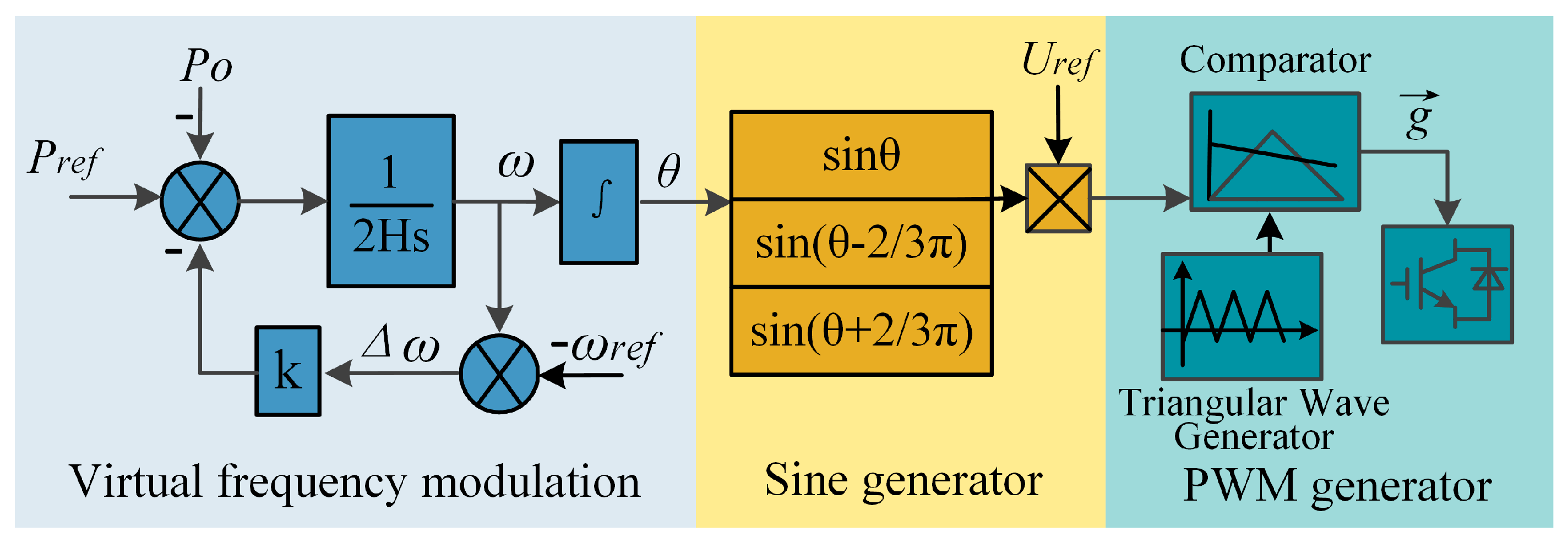
Figure 2.
Synchronous generator model.

Figure 3.
Representation of the electrostatic machine.
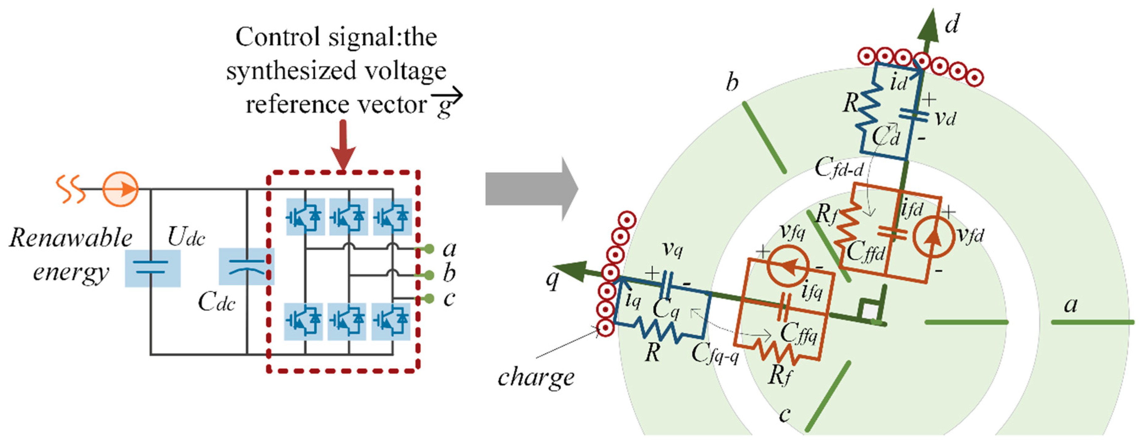
Figure 4.
The equivalent circuit of the IIDG system.

Figure 5.
Nonlinear VSG-IIDG model.

Figure 6.
satisfying the Popov condition on the complex plane.
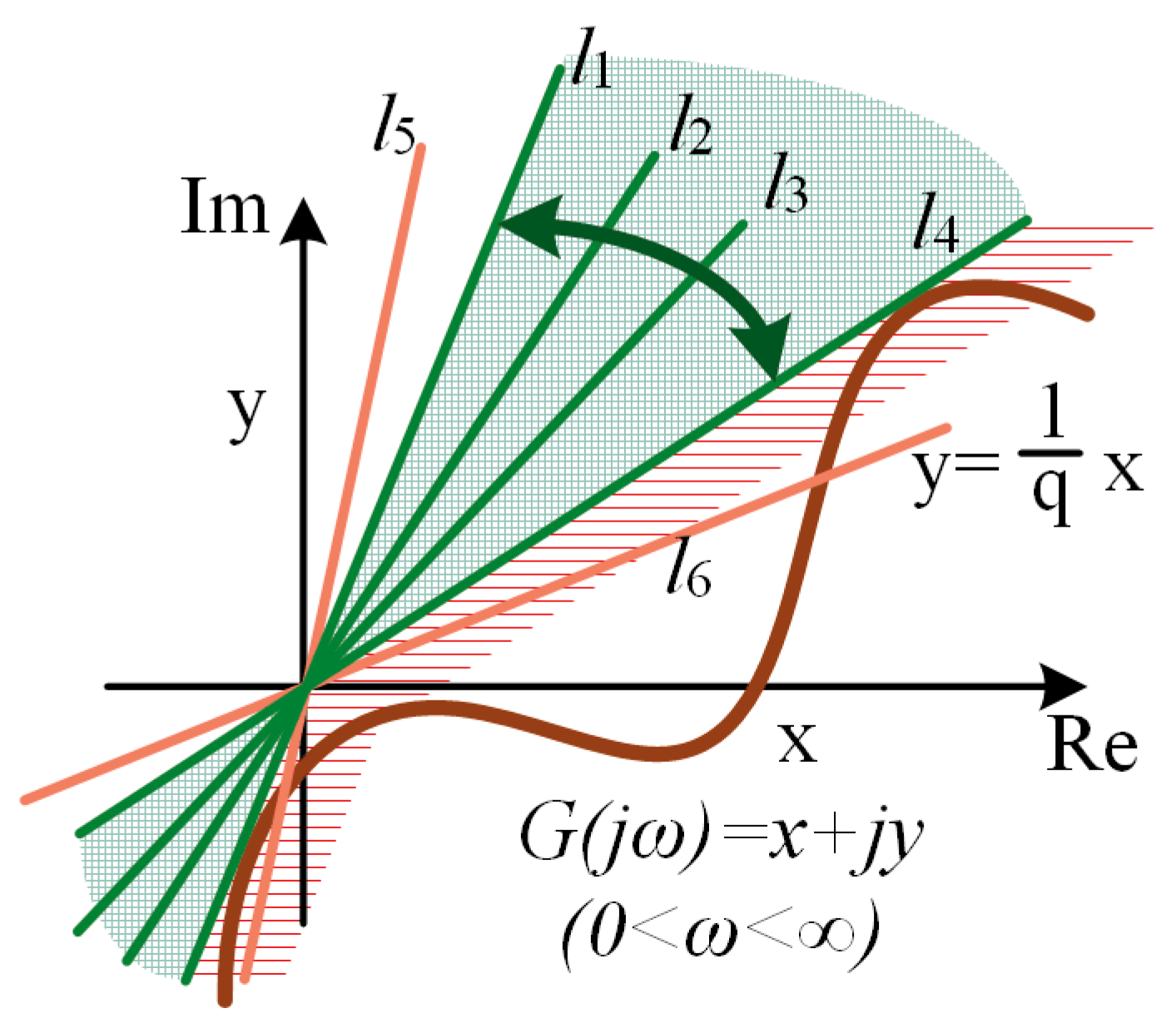
Figure 7.
Contour plots of V function.

Figure 8.
Operational trajectories of stable points.

Figure 9.
Comparison of simulations when fault clearing time are different. (a) Operational trajectories; (b) Angle difference; (c) Angular frequency of the IIDG.
Figure 9.
Comparison of simulations when fault clearing time are different. (a) Operational trajectories; (b) Angle difference; (c) Angular frequency of the IIDG.
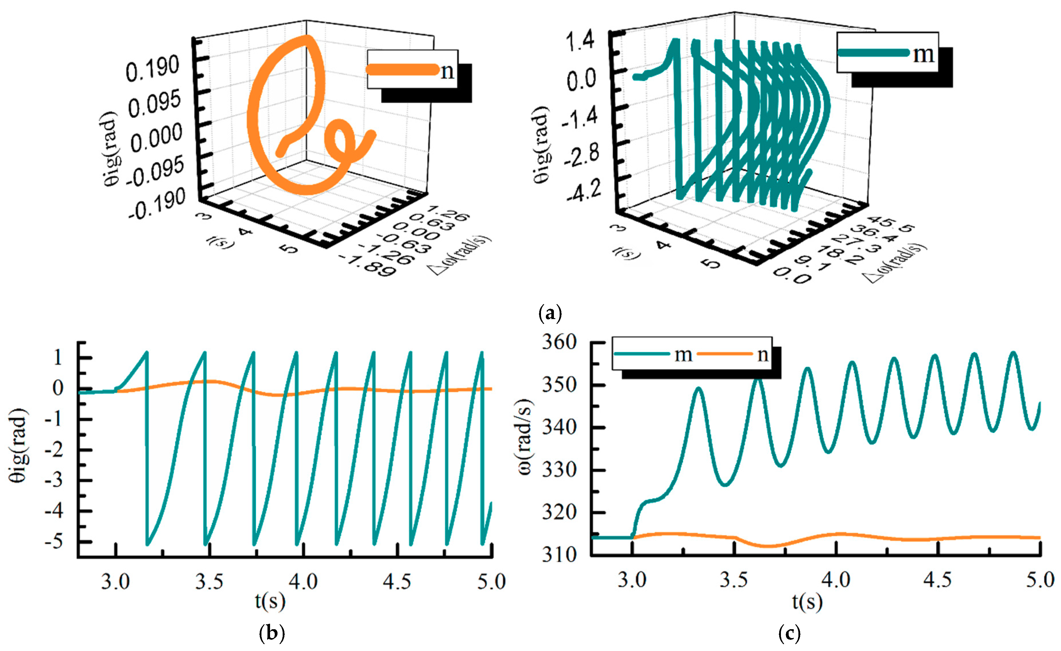
Figure 10.
The stability domain. (a) Under different impedance of cable; (b) Under different load power; (c) Under different virtual inertia.
Figure 10.
The stability domain. (a) Under different impedance of cable; (b) Under different load power; (c) Under different virtual inertia.

Table 1.
Rules and steps of the stability domain determination.
| Step 1 | Input the parameters: voltage, current, control parameters as H, k, etc. |
| Step 2 | Obtain the expression of output power as Equation (27) |
| Step 3 | Calculate the equilibrium point as Equation (4) |
| Step 4 | Establish Lyapunov function V() as Equation (18) |
| Step 5 | Figure out the critical stability energy M as Equation (19) |
| Step 6 | If V() < M, the system is large signal stable |
Table 2.
Parameters of the VSG-IIDG and control system.
| Parameters | Value |
|---|---|
| DC voltage | 1 kV |
| DC capacitance | 100 μF |
| Filtering capacitance | 400 μF |
| Filtering impedance | 1 mH |
| AC voltage | 311 V |
| Resistance of cable | 0.2 |
| Reactance of cable | 1 mH |
| Power of load | 300 kW + j100 kVar |
| Virtual inertia H | 0.15 |
| Damping factor k | 0.01 |
Table 3.
Stability of the VSG-IIDG with different , , and H.
| Load Power | Cable Impedance | Virtual Inertia H | Stability |
|---|---|---|---|
| 0.3 | 0.2 + j0.314 | 0.15 | stable |
| 0.6 | 0.2 + j0.314 | 0.15 | stable |
| 1 | 0.2 + j0.314 | 0.15 | unstable |
| 0.3 | 0.5 + j0.785 | 0.15 | stable |
| 0.3 | 1 + j1.57 | 0.15 | unstable |
| 0.3 | 0.2 + j0.314 | 0.5 | stable |
| 0.3 | 0.2 + j0.314 | 2 | unstable |
Table 4.
Sensitivity of the stability domain area to , , and H.
| (MW) | 0.1 | 0.3 | 0.5 | 0.7 | 0.9 |
| Sensitivity | −4.991 | −4.981 | −4.701 | −4.687 | −4.295 |
| (Ω) | 0.2 + j0.314 | 0.4 + j0.628 | 0.6 + j0.942 | 0.8 + j1.256 | 1 + j1.57 |
| Sensitivity | −5.661 | −5.508 | −5.138 | −4.037 | −4.011 |
| H | 0.1 | 0.5 | 1 | 1.5 | 2 |
| Sensitivity | −1.980 | −2.256 | −3.007 | −4.751 | −5.124 |
© 2018 by the authors. Licensee MDPI, Basel, Switzerland. This article is an open access article distributed under the terms and conditions of the Creative Commons Attribution (CC BY) license (http://creativecommons.org/licenses/by/4.0/).
Share and Cite
MDPI and ACS Style
Li, M.; Huang, W.; Tai, N.; Yu, M. Lyapunov-Based Large Signal Stability Assessment for VSG Controlled Inverter-Interfaced Distributed Generators. Energies 2018, 11, 2273. https://doi.org/10.3390/en11092273
AMA Style
Li M, Huang W, Tai N, Yu M. Lyapunov-Based Large Signal Stability Assessment for VSG Controlled Inverter-Interfaced Distributed Generators. Energies. 2018; 11(9):2273. https://doi.org/10.3390/en11092273
Chicago/Turabian StyleLi, Meiyi, Wentao Huang, Nengling Tai, and Moduo Yu. 2018. "Lyapunov-Based Large Signal Stability Assessment for VSG Controlled Inverter-Interfaced Distributed Generators" Energies 11, no. 9: 2273. https://doi.org/10.3390/en11092273
Note that from the first issue of 2016, this journal uses article numbers instead of page numbers. See further details here.