Resilience Assessment and Its Enhancement in Tackling Adverse Impact of Ice Disasters for Power Transmission Systems


1
State Key Laboratory of Disaster Prevention and Reduction for Power Grid Transmission and Distribution Equipment, Changsha 410129, China
2
State Grid Hunan Electric Company Limited Disaster Prevention and Reduction Center, Changsha 410129, China
3
School of Electric Power Engineering, South China University of Technology, Guangzhou 510640, China
*
Author to whom correspondence should be addressed.
Energies 2018, 11(9), 2272; https://doi.org/10.3390/en11092272
Submission received: 6 August 2018
/
Revised: 18 August 2018
/
Accepted: 21 August 2018
/
Published: 29 August 2018
(This article belongs to the Section F: Electrical Engineering)
Abstract
:Ice disasters have frequently occurred worldwide in recent years, which seriously affected power transmission system operations. To improve the resilience of power grids and minimize economic losses, this paper proposes a framework for assessing the influence of ice disasters on the resilience of power transmission systems. This method considers the spatial–temporal impact of ice disasters on the resilience of power transmission systems, and the contingence set for risk assessment is established according to contingency probabilities. Based on meteorological data, the outage models of power transmission components are developed in the form of generic fragility curves, and the ice load is given by a simplified freezing rain ice model. A cell partition method is adopted to analyze the way ice disasters affect the operation of power transmission systems. The sequential Monte Carlo simulation method is used to assess resilience for capturing the stochastic impact of ice disasters and deriving the contingency set. Finally, the IEEE RTS-79 system is employed to investigate the impact of ice disasters by two case studies, which demonstrate the viability and effectiveness of the proposed framework. In turn, the results help recognize the resilience of the system under such disasters and the effects of different resilience enhancement measures.

1. Introduction
Extreme events [1,2,3], which are low-probability high-impact, may cause a significant damage to the operational resilience of a power system, leading to wide-area power outages. As a key element in the critical infrastructure of a modern society, a power system should be not only reliable during a typical power system outage, but also resilient to extreme events. The effect of ice disasters is increasingly serious on transmission systems, such as the ice storm, which happened in January 1998, hit Eastern Canada and the Northeastern United States and caused 1.4 million households to be affected by power blackouts [4]. Another example is the 2008 ice disaster in Southern China that wreaked havoc on power grid equipment and interrupted power supplies in disaster areas, knocking out more than 36,000 transmission lines and affecting 27 million households [2]. These outages reveal that power systems are in dire need of practical solutions to withstand such infrequent, low-probability high-impact events [5]. In terms of the impact of ice disasters on power systems, a two-state weather model [6] and a multi-state weather model [7] were developed and used for evaluating the weather impact on power systems. The Markov process [7,8] and Monte Carlo simulations [9,10,11] were widely employed to describe system behavior and evaluate the stochastic impact of weather under different weather conditions. To support the ice loads and predict ice cover thickness, physical methods [12], empirical methods [13,14], and intelligent methods [15] were introduced. The stable operation of overhead lines affected by ground wire breakage accidents was discussed in [16]. A technique for modelling ice storms was developed in [17], which was also applied to evaluate the impact of ice storms on the Swedish transmission network.
Traditionally, power transmission systems are designed in accordance with reliability requirements [18,19], which mainly concentrate on high-probability low-impact events. The conventional power transmission system planning schemes focus on the “N-1” or “N-2” criteria, which aim to ensure that loads of power transmission systems can be restored if a failure of single component or that of any two components occurs [20]. In practice, however, components may suffer a cascading failure when power systems face extreme disruptive disasters; for example, hurricane Sandy is an “N-90” contingency [21]. Therefore, under such disruptions, the security of power supply of a power transmission system is affected even though the reliability criteria are met. Regarding above issue, the concept of resilience is introduced and building a resilient power grid becomes a top priority [22].
The concept of resilience has been widely used in different fields, for instance, ecology [23], environmental science and technology [24,25], sociology [26,27], and economics [28]. Specifically, the resilience of power systems includes the following abilities during an extreme event: (i) recover and anticipate which events are low-probability high-impact, (ii) recover quickly to restore from these extreme events, (iii) absorb lessons that adapt operations and make enhancements to mitigate severe consequences of similar future events [29,30,31,32].
To analyze the resilience of a power system, various methodologies and resilience indexes were presented. Resilience in a transmission network was studied in [33], designing a probabilistic methodology to assess the resilience of power transmission systems under extreme weather conditions. The frameworks for analyzing the resilience of a power system with integrated micro-grids were presented in [34,35] and an enhancement method for improving wind power penetrated power systems’ resilience was introduced in [36,37]. A resilience assessment framework to measure the resilience of power distribution system was proposed in [38], which focused on the performance of customers. Refernce [22] thoroughly reviewed existing studies on resilience assessment and methods to improve resilience of power systems, and proposed a quantitative framework for the resilience evaluation of a power grid that considers resilient load restoration. With resilience indices as a key focus, Refernce [39] quantified resilience in a communication network by a radar plot. [33] used the loss of load expectation and frequency to quantify resilience. As depicted in Figure 1, the resilience triangle model [40,41] on the basis of system performances was widely used in the majority of studies [42,43,44], which does not consider the duration of extreme events to capture the evolution of disruptive events. Instead of using a resilience triangle model, Refernce [45] built the concept of a resilience trapezoid to analyze resilience and their characteristics, and their advantages and disadvantages were thoroughly discussed in [32].
In this paper, a methodology for evaluating the impact of ice disasters on the resilience of power transmission systems is proposed. The proposed methodology refreshes location and strength of ice storm dynamically while considering actual location of power transmission systems and track of ice storm. The conceptual resilience trapezoid is adopted to develop a resilience model and a modified resilience index (RICD) is constructed to quantify the resilience of power transmission systems. This methodology can be applied in a comparative study to assess the influence of different extreme events, which focuses on the characteristics of an extreme event, i.e., the intensity and duration of impacts. The fragility model of components is established to describe the numerical relationship between the failure probability and the weather intensity. Unlike the existing risk assessment method, the proposed method evaluates the impact of ice storm on power transmission systems using publicly available meteorological data. Both the space- and time- impacts of ice storm are investigated adopting a cell partition method and the sequential Monte Carlo simulation. By taking into account more factors, such as the weather intensity, the location of affected components and the emergency capacity, a restoration model of components is developed in the resilience assessment. Furthermore, unlike the conventional power system reliability evaluation, a power system response model is developed to consider multiple component outages, as well as system splitting, which can reflect real operation scenarios under extreme events.
This paper is organized as follows: Section 2 discusses the conceptual resilience trapezoid to describe the performance of a power system and a modified quantitative resilience metrics. Section 3 describes the proposed resilience assessment methodology, including a cell partition method, a fragility model of components, a restoration model of components, a power system response model, and an approach for resilience analyses. The proposed methodology is implemented, and different improvement measures are studied in Section 4. Finally, conclusion is given in Section 5.
2. Resilience Concept Model and Quantitative Resilience Metrics
2.1. Conceptual Resilience Trapezoid
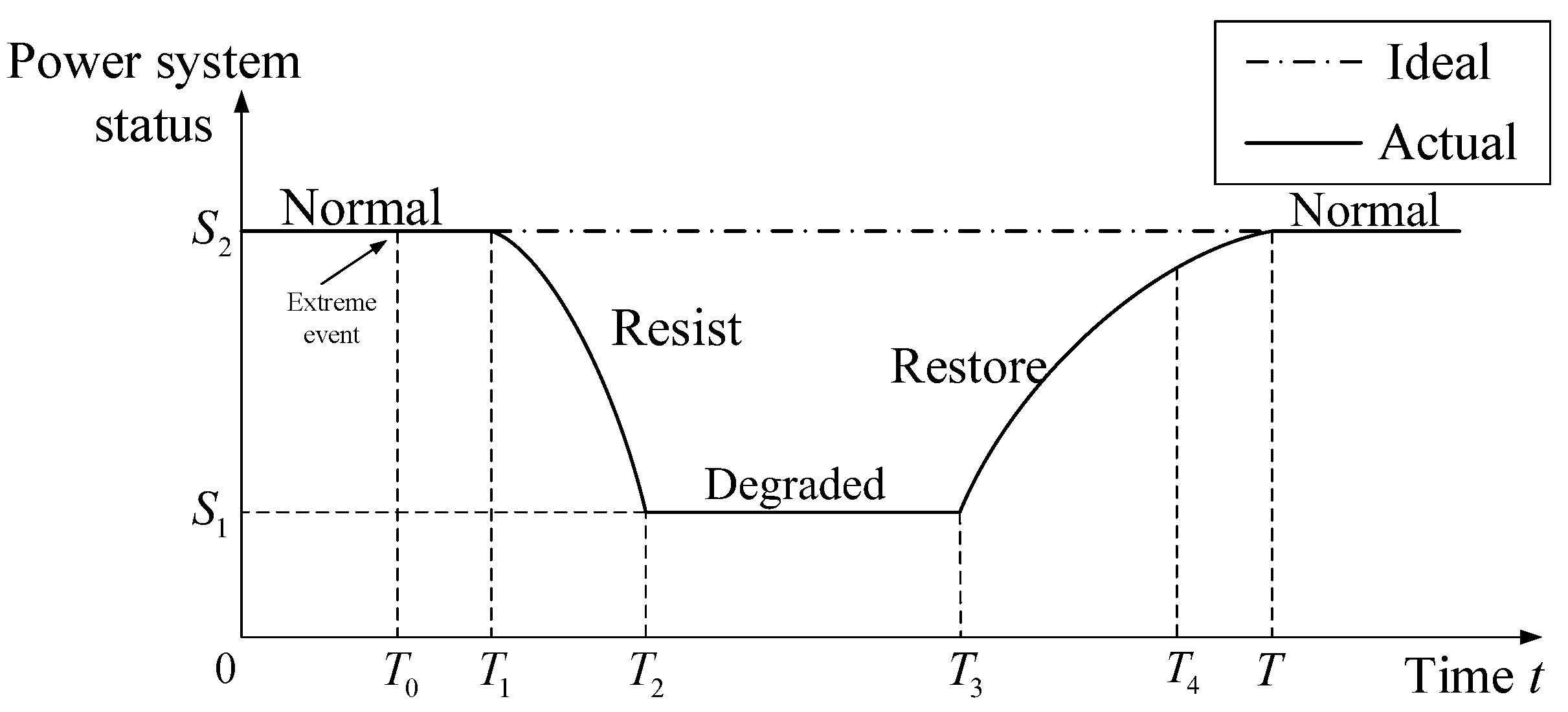
Traditionally, the resilience triangle is used to describe the performance of a power system associated with a disruption, which is only assessing the recovery performance of a electric power system following an extreme event, as shown in Figure 1. To propose a methodology for resilience assessment, a typical performance curve which depicts response processes of a power transmission system during an extreme event, as well as a conceptual resilience trapezoid are introduced. As shown as a time sequence, and the time dimension of the resilience curve is divided into five phases forming the following system resilience cycle: pre-disaster, disturbance, degraded, restorative, post-disaster.
As illustrated in Figure 2, the solid line is the actual system performance, the dotted line denotes the target performance. The relevant period is divided into five phases:
- Pre-disaster Phase: , illustrating that the system is in a normal working condition before the occurrence of a disruption. During the pre-disaster phase, advanced weather forecasts and disaster emergency decisions can be employed to anticipate and prepare for disruptive events.
- Disturbance phase: , representing that the system suffers from a disruption and the state degrades from to . In the disturbance phase, the system resists disruptive events, while the intensity of such disasters as typhoons and ice storms gradually increases. In other words, the system remains intact due to the small impact of disasters during . If a disaster has a huge initial impact, then moves to .
- Degraded phase: , showing that the system is degraded and stays in a decision-making period for resilience enhancement measures. In the degraded phase, the power system responds and adapts to allow the restoration phase to commence quickly.
- Restoration phase: , illustrating that the recovery process of the system, which recovers to the original normal state at T. In the restoration phase, the recovery capabilities of power system are limited by the manpower and restoration resources based on the actual situation. Therefore, the recover rate and time point of performance curve would be different (which are determined by the weather intensity, the location of damaged components, the size of the repair crew, and the contingency strategies) and discussed in Section 3.3.
- Post-disaster phase: , illustrating the system following the end of a extreme event. The post-disaster phase appears to contain a portion of restoration phase, as well as the terminal moment of restoration phase (T).
2.2. Resilience Indices
According to the conceptual resilience trapezoid model, the modified resilience index (RICD) is used to quantify the resilience, as shown in (1), which is based on the the mean ratio of the areas between the power system actual performance curve and the time axis and between the power system ideal performance curve and the axis within the period . RICD [46] is feasible in terms of both comparability and normalization, which quantifies the disruption impacts of an extreme event on a target system considering both the intensity and duration of impacts. Moreover, its formula contains the normal operation period , which can reflect the resistance ability of a target system against an extreme event.
where, and are the expected value and expectation, respectively. is the actual performance curve of a power system and is the performance curve of an undisturbed power system which in an ideal situation. denotes the duration of impacts of ice storm, that is . represents the probability of occurrence of fault scenario k and K is the total number of fault scenarios.
3. Resilience Assessment of Transmission Network to Ice Disasters
3.1. Cell Partition Method
Similar to the raster data used in geographic information systems, a transmission network is partitioned into a number of units by a cell partition method for assessing the spatial impact of ice disasters. The view of a power grid after applying the cell partition method is shown in Figure 3. The dimensions of each cell are equal both horizontally and vertically. The same weather condition is assumed within each cell. As a result, the impact of ice storm on transmission networks is capture by the performance of the partitioned system in every cell. The simulation step of ice disaster moving paths depends on the size of the mesh dimensions [35], which can be adjusted to a suitable spatial resolution with respect to accuracy requirements.
3.2. Fragility Model of Components
The concept of fragility curve [11,33,47] is adopted to model the vulnerability of a power transmission system under different weather intensities, which describes the relationship between the weather intensity and the failure probability of a component in a power transmission system, e.g., ice thickness. The fragility curve of component is shown in Figure 4, which denotes , i.e., the failure probability of a component of a power transmission system as a function of the weather intensity, and it can be written as follows:
where is the probability of a component failure and w is the weather intensity.
As ice disasters are the object of the resilience assessment, the weather intensity is denoted by the ice thickness to obtain the failure probability of components. A freezing rain ice accretion model [13] is used to calculate the ice loads based on meteorological data, which is shown below,
where represents the ice thickness, P and L denote the precipitation rate and the liquid water content, respectively. Let . H denotes the hours of freezing. and are the density of ice and water with and , respectively. V is the wind speed.
The impact of an ice disaster is not only determined by its intensity, but also the duration of the ice disaster upon a transmission system. Figure 5 shows the duration of the impacts of ice disaster on a landfalling region of transmission system (G). The duration of the impact can be determined by the path of the ice storm and the storm moving speed. and are the centers of an ice storm, which demonstrate the beginning and end locations of an ice storm affecting G, respectively. and are the radiuses of impact.
By obtaining the weather intensity, the failure probability of components () can be determined. If , the component is considered as breaking down, where r is a uniformly distributed random number (). If , the component will not break down. There is only consider the permanent fault in this research.
3.3. Restoration Model of Components
The restoration time is generated when a component of a transmission system experiences an outage, which is dependent on the weather intensity, the location of the damaged component, the size of the repair crew and the contingency strategies, as depicted in the follow principles:
- Considering the weather intensity: Under various weather situations, the durations for performing repairs are different. A time to repair (TTR) varible that increases with weather intensity is used, as shown in (4), which expresses the difficulty in restoring the fault components and the increasing degree of damage to the components caused by non-normal weather.where and are the repair time of components under normal weather and non-normal weather, respectively, is a multiplication factor as discussed in Section 4.In addition, TTR includes the following two aspects: (1) the time that the repair crew is dispatched from the department to a repair site (); (2) the repair time of damaged components (), it can be depict as.
- Regarding the location of the fault: is proportional to the distance between the damaged component and the departure location of the repair crew (s), and is inversely proportional to the moving speed of the repair crew (), as.
- Considering the size of the repair crew and the contingency strategies: In practice, the size of the repair crew is limited. It is possible that a large number of component outages occur in a catastrophic event, and there is not enough manpower for repairs. Based on the emergency response plan, components are repaired in order of priority. Hence, the time of a damaged component waiting to be repaired () should be take into consideration as in (7).
3.4. Power Systems Response Model
In extreme weather events, a power grid suffers from grid splitting and forms several sub-grids when multiple component outages occur. According the DC power flow model, the response model in this research is modeled as follows:
- In each sub-grid, if there is no power supply, then all load buses are considered to be failed;
- In the cases where the power supply in each sub-grid overrides the load demand, then the outputs of power plants are tailored to balance the generation and load demand. In the cases where there is a violation of the line flow constraints, load shedding is performed until the line power flow constraints are met and make sure the smallest number of consumer are affected. The dispatch commands are guided by the outcome of DC optimal power flow (OPF) calculation;
- In the cases where the load demand overrides power generation in each sub-grid, then the smallest amount of load is shed to achieve the generation and load demand balance. Meanwhile, the dispatch method is the same as that of Step 2.
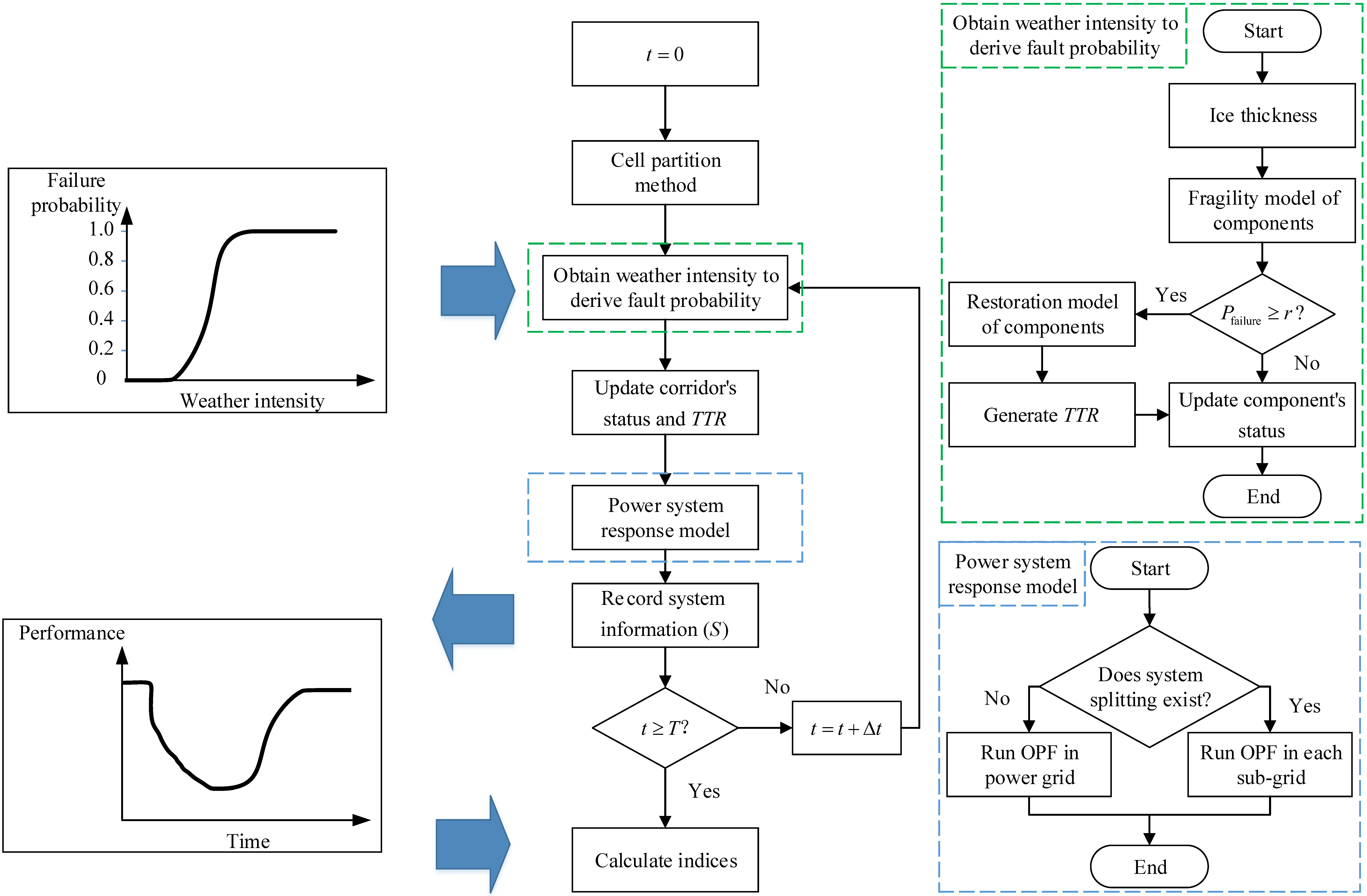
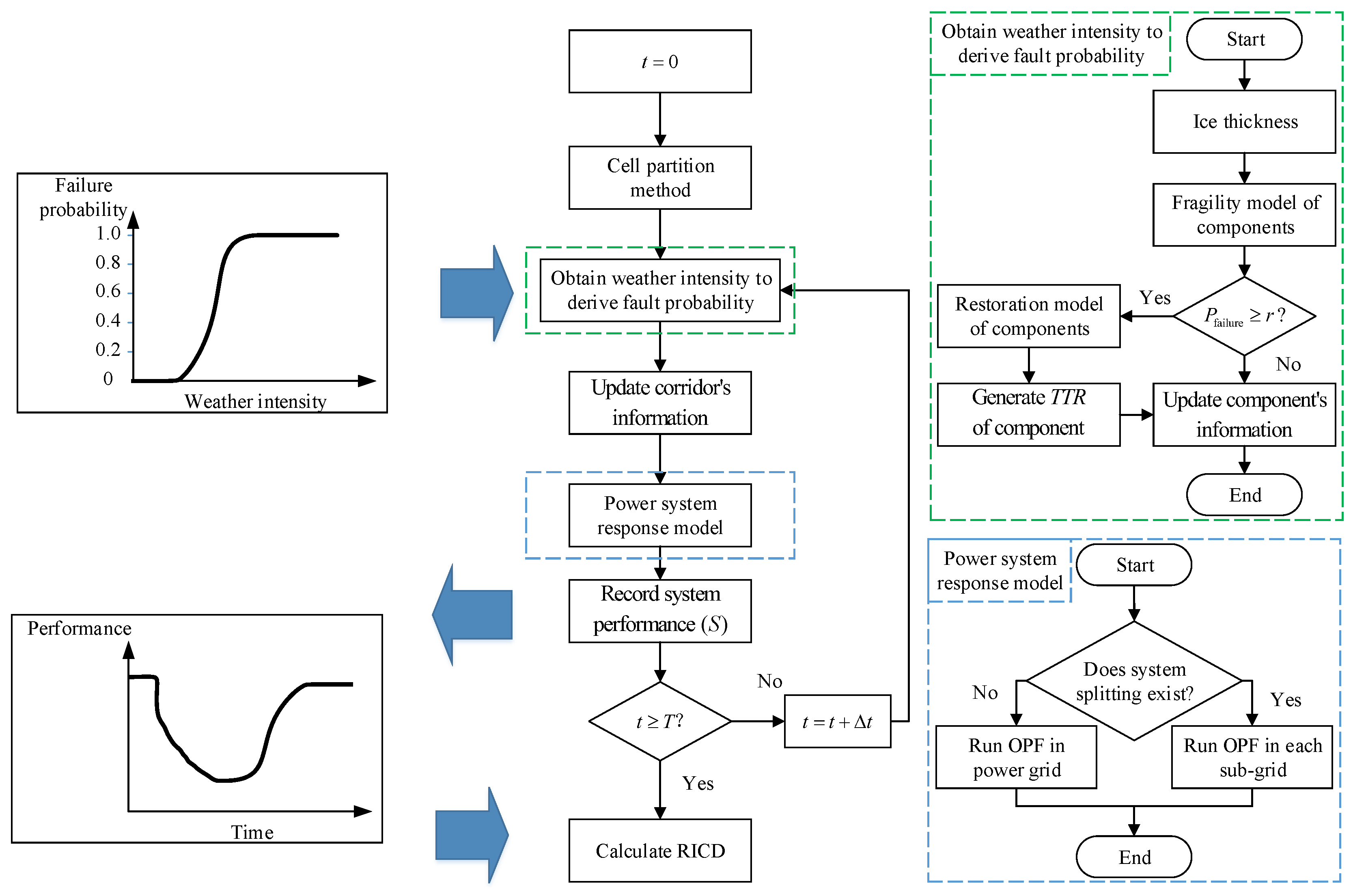
As an ice storm moves across a power transmission system, the sequential Monte Carlo simulation and the cell partition method (Section 3.1) are used to capture the multi-spatial and multi-temporal impact of the front of an ice disaster. The proposed methodology for resilience analysis to ice disasters is shown in Figure 6. Let the simulation step be , and the termination time be T. By acquiring the weather intensity of each region, the failure probabilities of components () are generated by the outage model (Section 3.2).
3.5. Methodology for Resilience Analysis
In each step , of all components are obtained and compared with r. If , then the component is considered to have experienced a breakdown. It is important to note that the conditions of adjacent components are not considered in this research. If a component breaks down, TTR is generated by the power system restoration model (Section 3.3). A power system response model (Section 3.4) is adopted to assess the system performance (S), which denoted by the load of system in this research.
Repeat the above procedures at every step and record the system information (S) in each step, to generate the system status curves of resilience. The process in which an ice disaster influences impacts a power transmission system is called an event, which is denoted as e. An event does not stop until (i) a disaster (such as ice) leaves the transmission system and (ii) the system recover to its original state. To calculate the resilience indices, the resilience index is calculated according to (1).
4. Numerical Examples, Results and Discussions
In this section, an ice disaster is simulated for the IEEE RTS-79 system [48], which is used to verify the proposed methodology for resilience evaluation regarding power transmission systems.
4.1. Test System and Simulation Data
The IEEE RTS-79 system contains 24 buses and 38 transmission lines as shown in Figure 7, and the ice load is assumed to be exerted on transmission lines in open air in this study. The generation system includes 32 units, which range from 12 to 400 MW. The peak load for the IEEE RTS-79 system is 2850 MW. To illustrate the spatial impacts of an ice storm and simplify the calculation process, the IEEE RTS-79 system is divided by a cell partition method, which partitions the studied areas into a number of cells with 2,880,000, as shown in Figure 8. In Figure 8, each cell presents the geographic area with , which can be represented by its coordinates in the format of Cell(x, y). The coordinates of the cell indicate where each bus is located, are listed in Table 1. The weather intensity and geographical position can be considered as the same in each cell if the dimensions are small enough.
The radius of the icing impact is 100 km. The moving speed of the ice storm C is 50 km/h. The maximum precipitation rate and maximum wind speed are 35 mm/h and 12 m/s, respectively. The path of ice storm in Figure 8 begins from Cell(230, 440) to Cell(1360, 1570).
Each cell is treated as the basic unit of the system, in which the vulnerability of a transmission power system is analyzed under an ice disaster. A fragility curve is displayed in Figure 4, in which the x-axis is denoted by the ice thickness in this example. Power transmission systems are usually designed to operate under certain conditions of ice thickness (M). When the ice thickness of a component (m) is less than or equal to the designed ice thickness M, the failure probability is set at 0; when , the ice thickness reaches the maximum tolerable intensity of the component, and the failure probability is consider as 1; and when , the failure probability rises with the increase of the ice thickness, which could be depicted by an exponential function. The estimation is more accurate with the availability of empirical data to make adjustments. M is set at 15 mm in this example. The fragility curve that considers icing is expressed as below [49],
of a transmission corridor in a cell is assumed as being 1 h, which can also be adjusted using empirical data. There are only twenty teams that handle the repair of a power transmission system. The moving speed of the crew is set as 60 km/h and the department of the repair crew is located at Cell(300, 700). When the supply of repair staff are not sufficient, the repair work of corridor is arranged in the order of line numbers, i.e., L1 > L2 > L3 ... > L37 > L38 as shown in Figure 7. The multiplication factor is uniformly and randomly generated considering the weather intensity as follows:
where U is a uniform distribution function.
4.2. Simulation and Results
4.2.1. Base Case: System Resilience Assessment
In this case, the system, whose simulation data are the same as discussed in the previous assumptions, is assessed by the proposed resilience assessment methodology. The ice thickness of the cells, where the part of the bus (BUS 3, BUS 5, BUS 7, BUS 14 and BUS 22) is located, is shown in Figure 9. Ice melt is not considered in this example. The cells containing BUS 5 and BUS 7 do not have icing, which are far away from the path of an ice storm and are outside the area impacted by this ice storm. The cells containing BUS 3, BUS 14 and BUS 22 occur icing, and their curves reach a maximum and remain there until the ice storm moves away. The maximum and the start time of icing cover are determined by the path and density of the ice storm and the location of the cell.
Figure 10 illustrates the result of the performance curve of the test system under the ice storm. The curve provides as 0.12 h, as 11.03 h, and . Moreover, it shows that the curve declined at , which is later than . When , the load of system is minimum as 2642.1 MW, which is reduced to 92.7% of its original normal state. This reveals that the system experienced large degradation when facing the ice storm, during , and the repair continues as well. After the end point of ice storm impact (), the load of system recovers to its normal value at , and finally the system state recovers to the original state at . There are still some failed components and their repair work continues between and T, and no violation of system constraints occurs after power rescheduling, so the system does not need to cut the load. From Figure 10, the resilience index is calculated by (1), and is 0.1635. The repair of the system in the Base Case, however, consumes too much time, resulting in a small .
4.2.2. Improvement Case: Comparing Different Improvement Measures
In this case, the resilience of the system in the Base Case is improved by three measures, namely enhancing the design standard of the system to be resistant of threats, improving the repair efficiency, and increasing the number of the repair crew.
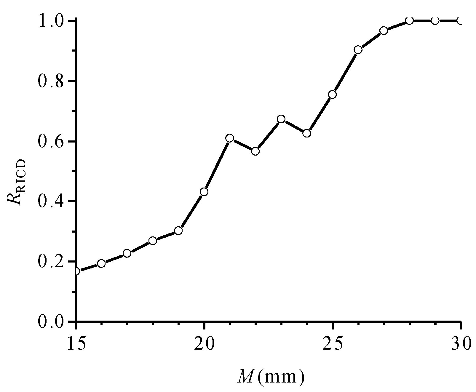
- Enhancing the design standard of the systemIn practical applications, the ice load exerted on the power transmission corridors may exceed the design strength of the material and cause component breakdown [33]. Enhancing the design standard for icing load can improve the resistance to icing load for components, for example the fragility curve is shifted to the right by improving design standards, as depicted in Figure 4 with dotted lines.Figure 11 demonstrates the resilience index at different designed icings of components. generally rises with the increase of M, except for when mm and mm. The reason for that is the output of is not only determined by the design standard of the system. The time of the failure and the order of the repair should also be considered. If , equals 1 when the designed icing of a component is larger than the ice storm intensity and no fault occurs.
- Improving the repair efficiencyVarious measures can be taken to raise the repair efficiency, e.g., increase diagnosis accuracy and shorten the time in determination of failure types and positions, improve the repair crew quality and skills, and reduce travel time. To reflect the change of under the different efficiency of the repair crew, the parameter e is introduced to represent the new () when the improvement measures are applied, i.e., . Figure 12 illustrates the system resilience under the different efficiency of the repair crew, which are represented by the relationship between and e. The curve on Figure 12 shows growing exponentially. equals 1 when , i.e., the damaged component is repaired instantaneously in an ideal situation.
- Increasing the number of repair crewFigure 13 demonstrates the relationship between and the number of repair crew, where the step of the X-axis variable is 10. The results show that increases with the increase of the number of repair crew and converges at 0.38 when its number exceeds 100. There is a limit for the improvement of the resilience, when the number of repair crew is increasing. The system performance is saturated if the repair crew can completely satisfy the demand for the damaged power transmission system.
Through the simulation results, the resilience enhancement measures in the Improvement Case appear to be able to improve the system resilience in the Base Case effectively. Different measures of improving the resilience have their special advantages, so the economic benefit, improving effect, and topology of the power transmission system must be considered in real applications for achieving comprehensive optimization.
5. Conclusions
This paper has proposed a dynamic methodology for assessing the impact of ice disasters on the resilience of power transmission systems, based on a modified resilience metrics (RICD) capable of effectively capturing the characteristics of extreme event. Moreover, the proposed methodology not only considers the geographical location of a grid, but also takes into account the path of an ice storm. The restoration model of components is developed by including the geographical location of a component, the weather intensity, the emergency, and the repair crew. While the power system response model is built to considered system splitting when facing extreme events. The results of numerical examples highlight the feasibility and efficiency of the proposed method in evaluating the resilience of a power transmission system under ice disasters, and reflect the contribution of improvement measures. Meanwhile, the assessment results can be used for further analysis to determine proper and the best improvement measures to improve the resilience of a power transmission system to withstand such ice disasters.
Author Contributions
J.L. guided the framework of the paper and provided professional guidance. J.G. and Z.J. provided professional guidance and collected all the data. Y.Y. did simulation and wrote the paper. W.T. provided the academic assistance and revised the manuscript.
Funding
This research was funded by Science and Technology Project of State Grid Electric Corporation (No. 5216A0180007) and Open Fund of State Key Laboratory of Disaster Prevention and Reduction for Power Grid Transmission and Distribution Equipment (No. SGHNFZ00FBYJJS1700041).
Conflicts of Interest
The authors declare no conflict of interest.
References
- Mimura, N.; Yasuhara, K.; Kawagoe, S.; Yokoki, H.; Kazama, S. Damage from the Great East Japan Earthquake and Tsunami—A quick report. Mitig. Adapt. Strateg. Glob. Chang. 2011, 16, 803–818. [Google Scholar] [CrossRef]
- Lu, J.Z.; Zeng, M.; Zeng, X.J.; Fang, Z.; Yuan, J. Analysis of Ice-Covering Characteristics of China Hunan Power Grid. IEEE Trans. Ind. Appl. 2015, 51, 1997–2002. [Google Scholar] [CrossRef]
- Mendonça, D.; Wallace, W.A. Impacts of the 2001 World Trade Center Attack on New York City Critical Infrastructures. J. Infrastruct. Syst. 2006, 12, 260–270. [Google Scholar] [CrossRef] [Green Version]
- Lecomte, E.L.; Pang, A.W.; Russell, J.W. Ice Storm’98; Institute for Catastrophic Loss Reduction: Toronto, ON, Canada, 1998. [Google Scholar]
- Venkata, S.; Hatziargyriou, N. Grid Resilience: Elasticity Is Needed When Facing Catastrophes [Guest Editorial]. Power Energy Mag. IEEE 2015, 13, 16–23. [Google Scholar] [CrossRef]
- Singh, C.; Billinton, R. System Reliability, Modelling and Evaluation; Hutchinson: London, UK, 1977. [Google Scholar]
- Billinton, R.; Singh, G. Application of adverse and extreme adverse weather: Modelling in transmission and distribution system reliability evaluation. IEE Proc. Gener. Transm. Distrib. 2006, 153, 115–120. [Google Scholar] [CrossRef]
- Billinton, R.; Singh, G.D. Reliability assessment of transmission and distribution systems considering repair in adverse weather conditions. In Proceedings of the IEEE CCECE 2002 Canadian Conference on Electrical and Computer Engineering, Winnipeg, MB, Canada, 12–15 May 2002; Volume 1, pp. 88–93. [Google Scholar]
- Bhuiyan, M.R.; Allan, R.N. Inclusion of weather effects in composite system reliability evaluation using sequential simulation. IEE Proc. Gener. Transm. Distrib. 2002, 141, 575–584. [Google Scholar] [CrossRef]
- Li, G.F.; Zhang, P.; Luh, P.B.; Li, W.Y.; Bie, Z.H.; Serna, C.; Zhao, Z.B. Risk Analysis for Distribution Systems in the Northeast U.S. Under Wind Storms. IEEE Trans. Power Syst. 2014, 29, 889–898. [Google Scholar] [CrossRef]
- Yang, Y.H.; Xin, Y.L.; Zhou, J.J.; Tang, W.H.; Li, B. Failure probability estimation of transmission lines during typhoon based on tropical cyclone wind model and component vulnerability model. In Proceedings of the 2017 IEEE PES Asia-Pacific Power and Energy Engineering Conference (APPEEC), Bangalore, India, 8–10 November 2017; pp. 1–6. [Google Scholar]
- Jiang, X.; Han, X.; Hu, Y.; Yang, Z. Model for ice wet growth on composite insulator and its experimental validation. IET Gener. Transm. Distrib. 2018, 12, 556–563. [Google Scholar] [CrossRef]
- Jones, K.F. A simple model for freezing rain ice loads. Atmos. Res. 1998, 46, 87–97. [Google Scholar] [CrossRef]
- Lenhard, R. An indirect method for estimating the weight of glaze on wires. Bull. Am. Meteorol. Soc. 1955, 36, 1–5. [Google Scholar] [CrossRef]
- Xu, X.; Niu, D.; Zhang, L.; Wang, Y.; Wang, K. Ice Cover Prediction of a Power Grid Transmission Line Based on Two-Stage Data Processing and Adaptive Support Vector Machine Optimized by Genetic Tabu Search. Energies 2017, 10, 1862. [Google Scholar] [CrossRef]
- Liu, G.; Guo, D.; Wang, P.; Deng, H.; Hong, X.; Tang, W. Calculation of Equivalent Resistance for Ground Wires Twined with Armor Rods in Contact Terminals. Energies 2018, 11, 737. [Google Scholar] [CrossRef]
- Brostrom, E.; Ahlberg, J.; Soder, L. Modelling of Ice Storms and their Impact Applied to a Part of the Swedish Transmission Network. In Proceedings of the Power Tech, 2007 IEEE Lausanne, Lausanne, Switzerland, 1–5 July 2007; pp. 1593–1598. [Google Scholar]
- Guo, L.; Guo, C.X.; Tang, W.H.; Wu, Q.H. Evidence-based approach to power transmission risk assessment with component failure risk analysis. Gener. Transm. Distrib. IET 2012, 6, 665–672. [Google Scholar] [CrossRef]
- Xie, K.G.; Cao, K.; Yu, D.C. Reliability Evaluation of Electrical Distribution Networks Containing Multiple Overhead Feeders on a Same Tower. IEEE Trans. Power Syst. 2011, 26, 2518–2525. [Google Scholar] [CrossRef]
- Li, W.Y. Risk Assessment of Power Systems: Models, Methods, and Applications; Wiley-IEEE Press: New York, NY, USA, 2005. [Google Scholar]
- Gholami, A.; Aminifar, F.; Shahidehpour, M. Front Lines Against the Darkness: Enhancing the Resilience of the Electricity Grid Through Microgrid Facilities. IEEE Electrif. Mag. 2016, 4, 18–24. [Google Scholar] [CrossRef]
- Bie, Z.H.; Lin, Y.L.; Li, G.F.; Li, F.R. Battling the Extreme: A Study on the Power System Resilience. Proc. IEEE 2017, 105, 1253–1266. [Google Scholar] [CrossRef]
- Holling, C.S. Resilience and Stability of Ecological Systems. Annu. Rev. Ecol. Syst. 1973, 4, 1–23. [Google Scholar] [CrossRef] [Green Version]
- Cutter, S.L.; Barnes, L.; Berry, M.; Burton, C.; Evans, E.; Tate, E.; Webb, J. A place-based model for understanding community resilience to natural disasters. Glob. Environ. Chang. 2008, 18, 598–606. [Google Scholar] [CrossRef]
- Li, Y.; Lence, B.J. Estimating resilience for water resources systems. Water Resour. Res. 2007, 43, 256–260. [Google Scholar] [CrossRef]
- Zobel, C.W.; Khansa, L. Quantifying Cyberinfrastructure Resilience against Multi-Event Attacks. Decis. Sci. 2012, 43, 687–710. [Google Scholar] [CrossRef]
- Zhong, S.; Clark, M.; Hou, X.Y.; Zang, Y.L.; Fitzgerald, G. Development of hospital disaster resilience: Conceptual framework and potential measurement. Emerg. Med. J. 2013, 31. [Google Scholar] [CrossRef] [PubMed]
- AdamRose. Economic resilience to natural and man-made disasters: Multidisciplinary origins and contextual dimensions. Glob. Environ. Chang. Part B 2007, 7, 383–398. [Google Scholar]
- Obama, B. Presidential Policy Directive 21: Critical Infrastructure Security and Resilience; The White House: Washington, DC, USA, 2013. [Google Scholar]
- Cabinet Office. Keeping the Country Running: Natural Hazards and Infrastructure; Cabinet Office: London, UK, 2011. [Google Scholar]
- Aitsi-Selmi, A.; Egawa, S.; Sasaki, H.; Wannous, C.; Murray, V. The Sendai Framework for Disaster Risk Reduction: Renewing the Global Commitment to People’s Resilience, Health, and Well-being. Int. J. Disaster Risk Sci. 2015, 6, 164–176. [Google Scholar] [CrossRef] [Green Version]
- Panteli, M.; Trakas, D.N.; Mancarella, P.; Hatziargyriou, N.D. Power Systems Resilience Assessment: Hardening and Smart Operational Enhancement Strategies. Proc. IEEE 2017, 105, 1–12. [Google Scholar] [CrossRef]
- Panteli, M.; Pickering, C.; Wilkinson, S.; Dawson, R.; Mancarella, P. Power System Resilience to Extreme Weather: Fragility Modeling, Probabilistic Impact Assessment, and Adaptation Measures. IEEE Trans. Power Syst. 2017, 32, 3747–3757. [Google Scholar] [CrossRef]
- Li, Z.; Shahidehpour, M.; Aminifar, F.; Alabdulwahab, A.; Al-Turki, Y. Networked Microgrids for Enhancing the Power System Resilience. Proc. IEEE 2017, 105, 1–22. [Google Scholar] [CrossRef]
- Liu, X.; Shahidehpour, M.; Li, Z.; Liu, X.; Cao, Y.; Bie, Z. Microgrids for Enhancing the Power Grid Resilience in Extreme Conditions. IEEE Trans. Smart Grid 2017, 8, 589–597. [Google Scholar]
- Liu, Y.; Wu, Q.; Zhou, X. Co-ordinated multiloop switching control of DFIG for resilience enhancement of wind power penetrated power systems. IEEE Trans. Sustain. Energy 2016, 7, 1089–1099. [Google Scholar] [CrossRef]
- Liu, Y.; Xiahou, K.; Lin, X.; Wu, Q. Switching Fault Ride-Through of GSCs Via Observer-Based Bang-Bang Funnel Control. IEEE Trans. Ind. Electron. 2018, 1. [Google Scholar] [CrossRef]
- Kwasinski, A. Quantitative Model and Metrics of Electrical Grids’ Resilience Evaluated at a Power Distribution Level. Energies 2016, 9, 93. [Google Scholar] [CrossRef]
- Erdene-Ochir, O.; Kountouris, A.; Minier, M.; Valois, F. A New Metric to Quantify Resiliency in Networking. IEEE Commun. Lett. 2012, 16, 1699–1702. [Google Scholar] [CrossRef]
- Bruneau, M.; Reinhorn, A. Exploring the Concept of Seismic Resilience for Acute Care Facilities. Earthq. Spectra 2007, 23, 41–62. [Google Scholar] [CrossRef]
- Tierney, K.; Bruneau, M. Conceptualizing and measuring resilience: A key to disaster loss reduction. Tr News 2009, 250, 14–17. [Google Scholar]
- Cimellaro, G.P.; Reinhorn, A.M.; Bruneau, M. Framework for analytical quantification of disaster resilience. Eng. Struct. 2010, 32, 3639–3649. [Google Scholar] [CrossRef]
- Ouyang, M.; Dueñas-Osorio, L.; Min, X. A three-stage resilience analysis framework for urban infrastructure systems. Struct. Saf. 2012, 36–37, 23–31. [Google Scholar] [CrossRef]
- Ouyang, M.; Dueñas-Osorio, L. Multi-dimensional hurricane resilience assessment of electric power systems. Struct. Saf. 2014, 48, 15–24. [Google Scholar] [CrossRef]
- Panteli, M.; Mancarella, P.; Trakas, D.N.; Kyriakides, E.; Hatziargyriou, N.D. Metrics and Quantification of Operational and Infrastructure Resilience in Power Systems. IEEE Trans. Power Syst. 2017, 32, 4732–4742. [Google Scholar] [CrossRef]
- Yang, Y.H.; Tang, W.H.; Liu, Y.; Xin, Y.L.; Wu, Q.H. Quantitative Resilience Assessment for Power Transmission Systems Under Typhoon Weather. IEEE Access 2018, 6, 40747–40756. [Google Scholar] [CrossRef]
- Jufri, F.H.; Kim, J.S.; Jung, J. Analysis of Determinants of the Impact and the Grid Capability to Evaluate and Improve Grid Resilience from Extreme Weather Event. Energies 2017, 10, 1779. [Google Scholar] [CrossRef]
- Subcommittee, P.M. IEEE Reliability Test System. IEEE Trans. Power Appar. Syst. 1979, PAS-98, 2047–2054. [Google Scholar] [CrossRef]
- Mei, S.W.; Xue, A.C.; Zhang, X.M. Self-Organized Critical Characteristics of Power Systems and Security of Power Grids; Tsinghua University Press: Beijing, China, 2009. [Google Scholar]
Figure 1.
The resilience triangle [41].
Figure 1.
The resilience triangle [41].

Figure 2.
The resilience trapezoid.

Figure 3.
Cell partition view of the power grid in Hunan Province, China.

Figure 4.
The fragility curve of component.

Figure 5.
The duration of the impact of an ice storm when making landfall on a transmission system.

Figure 6.
The proposed methodology for resilience analysis under ice disasters.

Figure 7.
IEEE RTS-79 System.

Figure 8.
The results of the cell partition method.

Figure 9.
The ice thickness of the cell part containing BUS 3, BUS 5, BUS 7, BUS 14 and BUS 22.

Figure 10.
The performance curve of target power transmission system under ice disasters.

Figure 11.
The resilience index at different designed icing load of the test system.

Figure 12.
The resilience index under the different efficiency of the repair crew.

Figure 13.
The resilience index at different number of repair crews.


Table 1.
Bus coordinates(Partial).
| Bus | 1 | 2 | 3 | 4 | 5 | 6 | 7 | 8 | 9 | 10 | 11 | 12 |
|---|---|---|---|---|---|---|---|---|---|---|---|---|
| x | 430 | 860 | 450 | 550 | 890 | 1300 | 1150 | 1230 | 800 | 1070 | 800 | 1075 |
| y | 180 | 110 | 700 | 410 | 350 | 420 | 190 | 310 | 700 | 650 | 870 | 850 |
© 2018 by the authors. Licensee MDPI, Basel, Switzerland. This article is an open access article distributed under the terms and conditions of the Creative Commons Attribution (CC BY) license (http://creativecommons.org/licenses/by/4.0/).
Share and Cite
MDPI and ACS Style
Lu, J.; Guo, J.; Jian, Z.; Yang, Y.; Tang, W. Resilience Assessment and Its Enhancement in Tackling Adverse Impact of Ice Disasters for Power Transmission Systems. Energies 2018, 11, 2272. https://doi.org/10.3390/en11092272
AMA Style
Lu J, Guo J, Jian Z, Yang Y, Tang W. Resilience Assessment and Its Enhancement in Tackling Adverse Impact of Ice Disasters for Power Transmission Systems. Energies. 2018; 11(9):2272. https://doi.org/10.3390/en11092272
Chicago/Turabian StyleLu, Jiazheng, Jun Guo, Zhou Jian, Yihao Yang, and Wenhu Tang. 2018. "Resilience Assessment and Its Enhancement in Tackling Adverse Impact of Ice Disasters for Power Transmission Systems" Energies 11, no. 9: 2272. https://doi.org/10.3390/en11092272
Note that from the first issue of 2016, this journal uses article numbers instead of page numbers. See further details here.