Impact of Drilling Costs on the US Gas Industry: Prospects for Automation

Sustainable Gas Institute, Imperial College London, 11 Princes Gardens, London SW7 1NA, UK
*
Author to whom correspondence should be addressed.
Energies 2018, 11(9), 2241; https://doi.org/10.3390/en11092241
Submission received: 2 August 2018
/
Revised: 20 August 2018
/
Accepted: 21 August 2018
/
Published: 27 August 2018
Abstract
:Recent low gas prices have greatly increased pressure on drilling companies to reduce costs and increase efficiency. Field trials have shown that implementing automation can dramatically reduce drilling costs by reducing the time required to drill wells. This study uses the DYNamic upstreAm gAs MOdel (DYNAAMO), a new techno-economic, bottom-up model of natural gas supply, to quantitatively assess the economic impact of lower drilling costs on the US upstream gas industry. A sensitivity analysis of three key economic indicators is presented, with results quoted for the most common field types currently producing, including unconventional and offshore gas. While all operating environments show increased profitability from drilling automation, it is found that conventional onshore reserves can benefit to the greatest extent. For large gas fields, a 50% reduction in drilling costs is found to reduce initial project breakevens by up to 17 million USD per billion cubic metres (MUSD/BCM) and mid-plateau breakevens by up to 8 MUSD/BCM. In this same scenario, additional volumes of around 160 BCM of unconventional gas are shown to become commercial due to both the lower costs of additional production wells in mature fields and the viability of developing new resources held in smaller fields. The capital efficiency of onshore projects increases by 50%–100%, with initial project net present value (NPV) gains of up to 32%.
1. Introduction
1.1. Drilling Automation
The exploration and production of hydrocarbon reserves is inherently expensive due to the high costs associated with drilling wells. To increase profitability at low gas prices, it is vitally important that the industry cuts the costs of both exploration and production. A study by the US Energy Information Agency (EIA) has shown that drilling accounts for a substantial proportion of both exploration and production costs [1]. For example, the development of Chevron’s Big Foot project required drilling and completion costs of around 1 billion USD, which was approximately a quarter of the project’s overall expenditure. A technology outlook study by DNV GL predicted that drilling automation will contribute significantly to reducing drilling costs by 2025 [2]. This prediction is not new, as automation has been suggested as a means of reducing drilling costs since at least the 1960s [3]. It has been suggested that the technology has not been adopted due to a lack of technical capability in automation and the oil industry’s use of day rate contracts [4]. Critics of drilling automation have claimed that it will reduce the ability of drilling crews to respond manually during emergency situations through the loss of skills. Similar issues have been faced by the airline industry and have been resolved through the use of simulation devices to prepare crews for automation failures. The implementation of automation is not predicted to completely eliminate drilling crews, but will act as a decision support system that directs the attention of drillers to where it is most required [5].
Studies have shown that drilling automation can decrease the time required to attain a targeted depth by around 30%–40%, by eliminating the interruptions that occur with traditional drilling methods [6,7,8]. By avoiding interruptions to the drilling process, the wellbore will be less likely to collapse and will avoid problems such as “stuck pipe” [9]. A type of drilling automation technology known as continuous drilling has been predicted to reduce drilling costs by 40%–45% and is currently undergoing field trials in Stavanger, Norway [10]. One study showed that the technology was able to increase the overall rate of penetration (ROP) for the first three wells drilled to 36 ft/hr (11.0 m/hr), which increased to almost 47 ft/hr (14.3 m/hr) for the next four wells drilled. This was an increase of around 30% over conventional methods. This ultimately led to a reduction in the time that the drilling rig was required on site by around 26% [11]. Safety on drilling rigs can also be greatly improved with automation, as it can reduce or even remove personnel from the drilling floor. The positioning and connection of drilling pipe is traditionally guided by manual labor, which exposes the drilling crew to the potentially fatal danger of being crushed by pieces of heavy drilling floor equipment [12].
The benefits of automated drilling technology have been summarized by Grinrod et al. [8] as follows:
- Significantly improved tripping speed.
- Significant improvement in time to run casing.
- Possibility of built-in continuous circulation and drilling.
- Improved personnel safety.
- Improved wellbore stability.
- Improved well safety.
- Avoidance of differential sticking.
- Lower power consumption.
- Less equipment wear.
Tripping speeds of 1800 to 3600 m/hr have been demonstrated in field trials, as have casing running speeds of 900 m per hour [8]. Both of these values exceed the “perfect well” speeds used as a theoretical maximum in the study by Brett [13,14], where the maximum theoretical tripping speed was estimated at 1645 m per hour and casing runs were estimated at 820 m per hour.
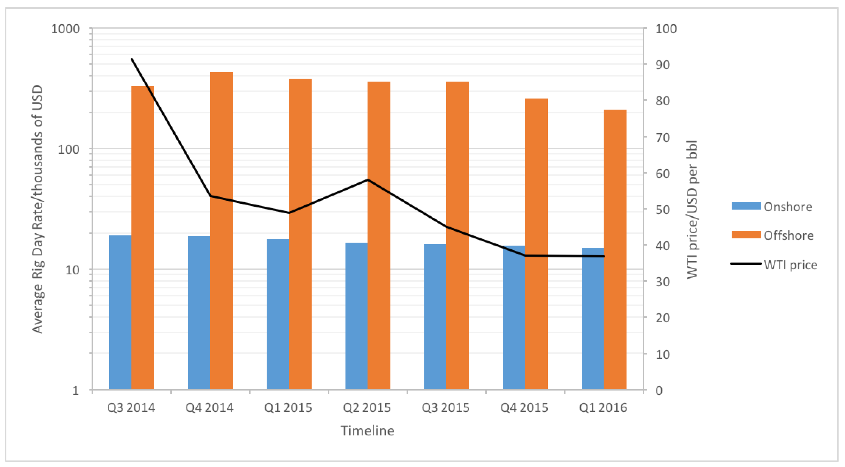
The vast majority of wells drilled across the world are undertaken by drilling contractors that supply both the rig and the crew. The efficiency of these operators is commonly measured by “nonproductive time,” which is defined as the time spent on activities that were unplanned and unnecessary. This is calculated as a percentage of the time taken to drill a well. As there are numerous other factors involved in the length of time it takes to drill a well, nonproductive time is not a reliable method of measuring the performance of different drilling projects [15]. Drilling contractors charge field operators for each day that they are required to drill wells based upon a pre-agreed day rate contract. Figure 1 shows cost estimates for rig day rates as a function of time. Offshore rig rates are around an order of magnitude greater than onshore. This is due to the substantial costs associated with operating at sea and the extensive support structure necessary for offshore personnel. The variation in day rate is similar for both onshore and offshore rigs and is primarily driven by supply and demand pressures, which are in turn driven by prevailing oil prices. The decline in day rates in late 2014 was a consequence of the collapse in oil prices that occurred around that time. Through 2015, offshore day rates dropped from 430,000 to 260,000 USD. Onshore day rates fell from 18,750 to 15,730 USD during the same period. Estimates of the cost of automated drilling equipment are not presently in the public domain, but it is likely to be offset by the reduction in drilling personnel costs and will have very little influence on the day rate cost relative to the oil price. The savings from implementing drilling automation will therefore come from the reduction in time spent drilling wells. Drilling contractors have little motivation to reduce drilling times other than competition with rival companies for contracts, which is not significant during periods when demand for their service outstrips supply. The lack of automation in the present-day drilling industry suggests that the policies required to encourage its adoption are not yet in place. It may be that the recent low oil price environment and the increased competition that this has created could be the critical factor that induces its adoption. This paper assumes that the recent predictions of its imminent adoption will prove correct and explores the economic benefits that could be achieved through the use of energy system modelling techniques.
Although continuous drilling can reduce costs by reducing the time it takes to drill, it is of course not immune to failure. Such failure may furthermore be harder to rectify due to indirect effects, such as the reduction in personnel actively overseeing operations [16]. Conversely, there is evidence that over a third of incidences of stuck pipe are attributable to drilling crew changeovers [17], which could be eliminated with automation. This study avoids the need for a detailed (and inevitably speculative) breakdown of cost savings and risks associated with continuous drilling by focusing on sensitivity to a single independent parameter, well capital expenditure (capex) relative to a business-as-usual reference scenario. In the scenarios presented, given savings in well capex should be interpreted as already including indirect costs from downtime due to failure and/or the cost of fixing equipment. For this reason, the findings of this study apply equally to any strategy that companies might employ to reduce drilling costs, with automation recognized as a likely important contributor, among others [18], in the near future.
1.2. Energy Systems Modelling
Energy systems models [4,5] are powerful tools for studying long-term transitions of energy systems and provide stakeholders with valuable information to inform decision-making about investments in new assets (in terms of capacity, type, and geographical context), technological R&D, and the likely impact of future climate change mitigation policies. They help stakeholders make reasoned investment decisions that are based upon quantitative data rather than opinion or speculation. The ModUlar energy systems Simulation Environment (MUSE) is a new open-access energy systems model being developed at Imperial College’s Sustainable Gas Institute [22] with a specific focus on understanding the role of natural gas in the future energy mix. MUSE is a global, technology-rich simulation of partial equilibrium across all energy vectors that seeks to combine engineering reality with a realistic treatment of investor behavior. Its modular structure facilitates a sophisticated treatment of the heterogeneous nature of energy supply and demand, with every sector (natural gas, coal, nuclear, renewables, etc.) modelled in a way most appropriate to its specific needs. On the supply side, one such module is the DYNamic upstreAm gAs MOdel (DYNAAMO) [23,24], a new dynamic simulation of the upstream gas industry. Although principally developed to interface with MUSE, DYNAAMO can run independently of MUSE and produce a range of technical, emissions-related, and econometric outputs that are of interest in their own right. In contrast to most “static” supply-side models, which bracket natural gas resources by cost, DYNAAMO generates dynamic supply curves by aggregating incremental supply on a subfield level, while incorporating realistic investment and operating decisions. DYNAAMO makes use of decades-long time series data [25] from thousands of gas fields worldwide to establish a realistic picture of both production and expenditure patterns over the life cycle of a typical field, including abandonment costs, the fiscal environment, and the costs of finding and developing additional resources. This detailed expenditure breakdown, in terms of both timing and type, makes DYNAAMO a useful tool for investigating the impact of new technologies on the upstream gas industry.
1.3. Methodology
To investigate the likely techno-economic consequences of drilling automation, we restrict our attention to the USA, for which there is a wealth of historic data that can be used to calibrate the model. Within the DYNAAMO framework, production is broken down by field environment, a combination of technology and operating environment with distinctive production and cost characteristics. Table 1 defines the 5 main field environments that can account for almost all natural gas production in the USA.
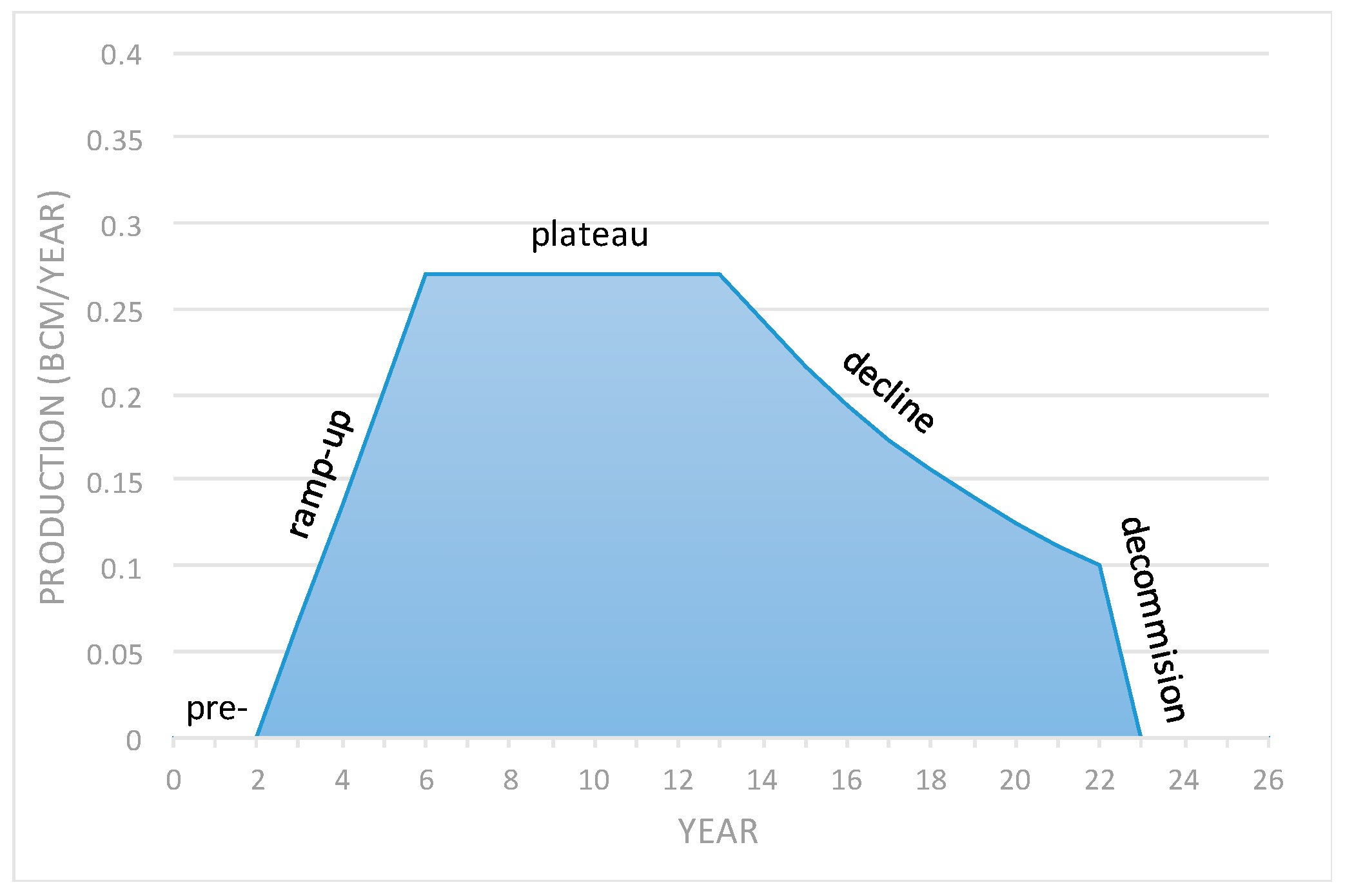
For each field environment, DYNAAMO constructs a prototypical field life cycle profile based on the 2P (The term “2P” stands for the sum of the proven and probable reserve estimates. A reserve is classified as proven if it is likely that 90% or more of that resource can be profitably recovered in the current economic climate. Probable reserves are deficient in geological data, making their presence and profitability uncertain. To compensate for this, the gross estimate is reduced by 50%.) estimated ultimate recovery (EUR) of the field. All aspects of the expenditure and production profile modelling are informed by historic data for US fields. Typical profiles are shown in Figure 2 and Figure 3. A reservoir follows standard preproduction, ramp-up, plateau, and decline phases [26], with the decline rate and abandonment time determined endogenously based on a reference forward price scenario, such that the anticipated total production equals the initial EUR. Large fields tend to produce a smaller fraction of their EUR per year on plateau than small fields, reflecting a trade-off between variable operational expenditure (opex) and the discounting of future cash flow. The result is that large fields normally produce over a longer period than small fields, although the field environment also plays a role, mainly due to the greater costs associated with offshore operations. Based on an analysis of historic production data [25], DYNAAMO uses a relationship of the form rate ~ EURy to model the plateau rate, with and for onshore and offshore fields, respectively (this is consistent with other modelling efforts [27]). As well as the production profile of a field, operational and capital expenditure (opex and capex) profiles vary considerably by field environment, reflecting both the relative importance of facilities and infrastructure costs in overall project financing and the timing and intensity of drilling. A detailed account of DYNAAMO’s approach to expenditure and production modelling can be found in [24].
Once the field life cycle profiles have been established, a range of economic and technical outputs can be calculated. This study focuses on 3 key outputs deemed most relevant to the economic evaluation of drilling automation:
• Initial net present value (NPV)
This is the field NPV at the start of the preproduction phase. It includes all future post-tax cash flow (including possible subsidies) discounted at 10% per annum based on a flat forward reference price for gas.
• Initial and midcycle breakeven price
This is the gas price for which the forward NPV = 0 at the start of preproduction and midway through the plateau phase, respectively. Breakevens can vary significantly over a project life cycle, depending on the field environment, reflecting the expected timing of positive and negative cash flow.
• Capital efficiency
This is a measure of expected return on capital, here taken as NPV per net present cost of capital (The cost of capital represents the opportunity cost of competing capital investments. It is contained in the rate used to discount capital expenditure, which in this report is set equal to the overall discount rate (10% per annum)) (including only discounted capex spent over the preproduction and ramp-up life cycle phases).
DYNAAMO was first run in the absence of automated drilling technology to create a business-as-usual (BAU) reference scenario. A forward gas price of 135 million USD per billion cubic metres (MUSD/BCM) (3.8 USD/MMbtu), corresponding to the average wellhead price during the period 2010 to 2015 [28], was used to calibrate production profiles against EUR, although the findings of this study are not significantly sensitive to the exact price chosen. The impact of automated drilling was then investigated in 5 scenarios in which the total project well capex was reduced from its BAU value by 10% to 50% in increments of 10%. Based on historic expenditure data, the percentage of total project capex allotted to drilling costs was taken to be 12%, 35%, 38%, 70%, and 70% for field environments 1 to 5, respectively (see Figure 4 and Table 1). Note that these estimates include drilling costs associated with primary, secondary, and tertiary recovery. The timing of drilling (and associated costs) also accounts for step-out and in-fill drilling, which typically occur toward the end of the plateau stage of production.
The field life cycle profiles (and therefore all consequent model outputs) depend on the initial 2P EUR. This varies enormously by individual field. However, data from several thousand historic and currently producing fields indicate that EUR is log-normally distributed, with a mean and variance characteristic of the particular field environment (see Figure 5). To model this diversity of field sizes, which can impact the economics of production via economies of scale, DYNAAMO samples the field size distributions to construct an asset class, a field of a specified field environment and characteristic size. The economic results quoted in this study are volume-weighted averages across asset classes.
2. Results
2.1. Breakeven Prices
The analysis assumes that the application of automated drilling can reduce drilling capex by up to 50%. Figure 6 shows a comparison of supply curves for US natural gas with and without automated drilling technology (here assumed to reduce well capex by the full 50%). DYNAAMO generates these by calculating the forward breakeven prices of producing fields, with each data point corresponding to a breakdown by asset class as well as the age of the field (life cycle year). Because the drilling profile depends heavily on the field environment, it is important to take into account the maturity of the field when estimating the impact of drilling automation on breakeven prices. The analysis shows that the application of drilling automation can reduce breakeven prices of the younger fields, as these will undergo the greatest quantity of drilling. The older fields tend to be large sandstone reservoirs that have already been drilled and will only require a small number of additional production wells to increase recovery. The younger fields tend to be tight/shale gas fields that require substantial drilling and can therefore benefit greatly from cost reduction. The modelled effect of drilling automation shifts the supply curve downward, but also to the right. This is a consequence of additional volume that becomes commercial to lift as a result of the technology. The effect is most pronounced during the decline phase of unconventional production, in which well capex is ongoing.
The area between the two lines is an estimate of the additional profit that can theoretically be obtained and was calculated to be 4364 MUSD (at a nominal forward price of 135 MUSD/BCM). The most expensive fields will be profitable only if gas prices rise substantially. For comparative purposes, the average Henry Hub price between 2010 and 2015 is also shown in Figure 6.
The breakeven price is the lowest price a rational producer will accept and still choose to continue operations. Breakeven prices are therefore often used to construct supply curves, but they also indicate how resilient the industry is to low price environments. Figure 7 shows the initial breakeven gas price as a function of well capex reduction. This is the breakeven price for a field commencing its preproduction phase. All five field environments can obtain a reduction in breakeven price by applying automated drilling technology. The cheapest field environments are deep offshore and CBM, as they primarily consist of large fields that require only a few production wells to be drilled throughout their operational lifetime. These types of field environment only began to be exploited in recent decades and, as such, the largest and best-quality reserves are presently being produced. In contrast, fields situated in the shelf region of the Gulf of Mexico have been heavily exploited in the past and only small reservoirs exist that are relatively expensive to produce. Opex is relatively consistent during a field’s lifetime, whereas production declines. This results in production costs increasing dramatically toward the end of operations. As shelf reservoirs are primarily sandstone, only a small number of production wells need to be drilled, with most of the cost coming from expensive topside production equipment. Tight/shale gas has the second highest breakeven price due to the high costs associated with horizontal drilling and fracking. The rapid depletion rate of tight/shale wells means that new wells are regularly required to maintain production levels. The large requirement for drilling also translates into greater cost reductions, as there is greater benefit realized from reduced drilling costs. Onshore conventional benefits to the greatest extent, as it has the highest initial breakeven price and therefore the greatest opportunity for gain. Recent onshore conventional discoveries tend to be smaller than unconventional fields, as the largest reserves were discovered and exploited decades ago. Recent discoveries therefore have a high capex-to-reserve ratio. A reduction in well capex will therefore benefit onshore conventional projects to the greatest extent. Figure 8 shows the breakeven prices for mature gas fields that are midway through the plateau stage of production illustrated in Figure 3. Midcycle breakevens are considerably lower than initial breakevens (producers will accept a lower price, given that most capital costs are already paid), yet only tight/shale and CBM benefit from drilling automation in this scenario, as the other field environments have completed the majority of the required drilling activity.
2.2. Net Present Value (NPV)
The net present value of different investment options is often used for comparative purposes when making investment decisions. Some exploration and production companies operate in multiple asset classes, and NPV analysis can be a useful method for estimating the optimal investment strategy [29]. Figure 9 shows variation in NPV as a function of well capex reduction. The analysis excludes fields with negative NPV, as these would not be produced. All field environments show an increase in NPV with increasing cost savings from drilling automation, with onshore conventional reserves showing the largest increase and offshore shelf the smallest. In comparing the impact of drilling cost reductions on NPV for conventional, unconventional, and offshore projects, several competing factors are at play. Onshore conventional reserves increase dramatically in value (and even more so in terms of capital efficiency; see Figure 10) because the capex associated with drilling takes place in the early stages of the project, in contrast to unconventionals, where it is spread over the project life cycle. However, unconventionals are far more drilling-intensive than conventionals (see Figure 4), suggesting that for unconventional reserves, the impact of cost reductions on NPV should also be significant. For shelf and deep offshore field environments, the production facilities capex is so large that a relatively smaller fraction of the total capex is spent on drilling and the increase in NPV is less pronounced. The low level of drilling involved in these field environments also limits the impact that automated drilling technology can have on profitability as a whole.
Both tight/shale and CBM have consistently higher NPVs relative to the other field environments. For tight/shale, the large size of the assets yields a consistently large NPV. For onshore conventional, only the largest fields have a positive NPV, and while these account for a relatively small proportion of asset classes within this field environment, they benefit greatly from the application of drilling automation.
2.3. Capital Efficiency
Capital efficiency is the ratio of net present value to discounted capital expenditure and is an indicator of risk, as it favors investments that require a lower capex to achieve a given return. Figure 10 shows capital efficiency as a function of well capex reduction. The analysis shows that capital efficiency is highest for the CBM field environment. While results will vary greatly according to the specifics of each well, CBM is an efficient use of capital, because the average size of the CBM fields is large relative to the other field environments.
The average field size of CBM is around six times greater than tight/shale in the USA, although there are presently far fewer fields. CBM fields are also generally cheaper to develop than tight/shale [25]. For example, a (typically sized) 10 BCM CBM field has an average capex per volume of 40.8 MUSD/BCM, whereas a tight/shale field of the same size has a capex per volume of 52.9 MUSD/BCM. CBM fields enjoy similar reductions in overall project opex. While there is significant variation, CBM fields are inherently cheaper to drill, as the typical depth of a CBM field is around 400 m, whereas tight/shale averages around 1500 m [30].
The well capex of unconventional resources such as CBM and tight/shale is spread out over the entire life of the field [25,30], whereas sandstone field environments tend to have most of their capital spent prior to commencing production. The time value of money therefore increases the capital efficiency of unconventional resources, as these typically involve smaller up-front capital financing. Capital efficiency is also greater due to the relative immaturity of unconventional natural gas. Its development will require extensive and continual drilling and is likely to be highly profitable as the best reserves are not yet exploited.
If drilling automation can reduce well capex by 50%, then this can improve capital efficiency to the extent that both onshore conventional and tight/shale can be economically competitive with deep offshore wells. The extensive drilling required by tight/shale means that drilling automation can greatly improve the project economics of these reserves.
Shelf production in the Gulf of Mexico shows virtually no change in capital efficiency due to the maturity of fields in this region. Production declined from 140 BCM in 2001 to 30 BCM in 2016 [31] and only a small quantity of production wells are expected to be drilled in the future. The offshore field environment shows the smallest improvement because well capex accounts for a smaller fraction of the total capex (i.e., facilities capex is large). The largest improvement is achieved for the onshore conventional field environment, as early-stage well capex can be reduced and the time value of money results in a large increase in NPV.
2.4. Wellhead Breakeven Price
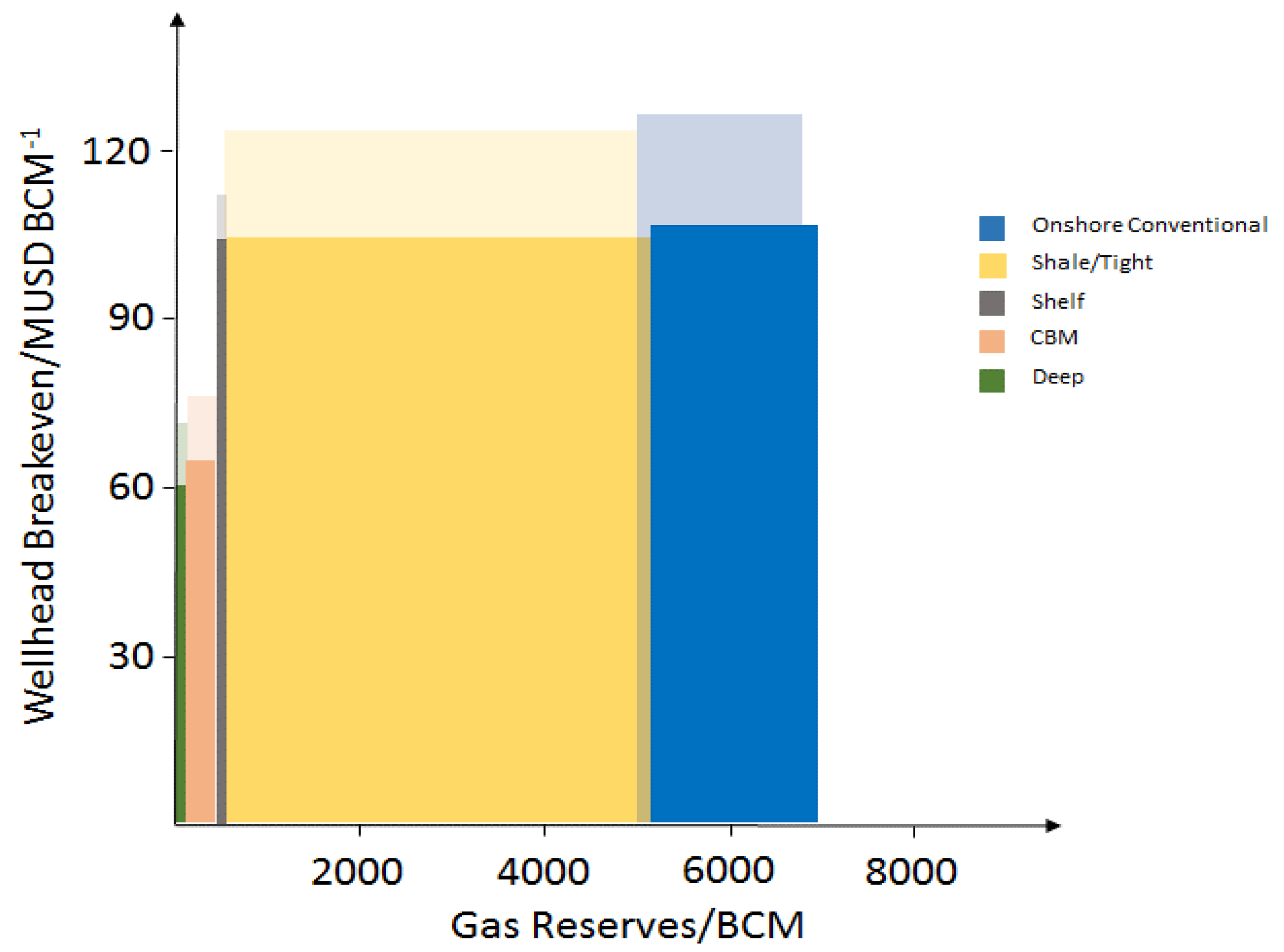
The wellhead breakeven price is a critical metric for assessing the value of different asset classes. It is an estimate of the cost of production but does not include transportation or processing costs. When these two factors are included, the wellhead breakeven price would be equal to the Henry Hub price. The wellhead and Henry Hub prices therefore track each other and vary relative to supply and demand. Figure 11 shows the wellhead breakeven price as a function of cumulative reserves. The data show that automated drilling is able to decrease the wellhead breakeven price for all field environments. Only the unconventional gas reserves of CBM and tight/shale show noticeable increases in reserve volume. This is because low-permeability gas reservoirs require extensive drilling to achieve economically viable flow rates and are at an early stage of their developmental life. Therefore a substantial quantity of drilling is required to develop these fields in the future. The figure also highlights how US gas reserves are presently dominated by tight/shale gas. Automated drilling is therefore especially important for the US gas industry, since this field environment is where the greatest quantity of drilling is required and automation can consequently have the greatest impact. Shelf and deep offshore environments presently account for a small percentage of reserves and are likely to decrease further as a consequence of their low NPV, as shown in Figure 9. There is a slight increase in the quantity of overall reserves of around 160 BCM.
3. Conclusions
The recent decrease in international oil and gas prices has led to a sharp reduction in demand for well-drilling services. Automation of the drilling process is expected to reduce drilling costs, with the fastest adopters of this technology likely to gain a competitive advantage over rival drilling companies.
This study sought to quantify the impact of drilling costs on the economics of the upstream gas industry. The USA was chosen as a case study, due to its diversity of production methods and the wealth of historic techno-economic data available. However, if regional fiscal considerations are accounted for, our findings should be relevant to natural gas production worldwide. We have shown that drilling costs play a significant role in determining the likely return on upstream investment. Every USD saved on drilling adds roughly 0.3 USD to initial NPV for large CBM fields and 0.75 USD for large deepwater fields. This study indicates that such savings also imply lower initial breakeven prices, with every 10 percentage point decrease in drilling costs lowering breakevens by 1.8–2.3 MUSD/BCM across all field environments. Significant reserve growth is likely to occur in tight/shale and conventional onshore fields, with modest additions for CBM plays. At current hub prices, it is estimated that adopting drilling automation is worth an additional 4.4 billion USD to the US gas industry as a whole.
Author Contributions
Conceptualization, D.J.G.C. and K.A.; Methodology, D.J.G.C. and K.A.; Software, D.J.G.C.; Validation, D.J.G.C., and K.A.; Formal Analysis, D.J.G.C. and K.A.; Investigation, D.J.G.C. and K.A.; Resources, A.D.H. and N.B.; Data Curation, D.J.G.C. and K.A.; Writing-Original Draft Preparation, D.J.G.C. and K.A.; Writing-Review & Editing, D.J.G.C., K.A., A.D.H. and N.B.; Supervision, A.D.H. and N.B.; Project Administration, A.H. and N.B.; Funding Acquisition, A.D.H. and N.B.
Funding
This research was funded by Natural Environment Research Council, grant number NE/N018656/1.
Acknowledgments
This work is supported Royal Dutch Shell plc via funding of the Sustainable Gas Institute at Imperial College London.
Conflicts of Interest
The authors declare no conflict of interest.
References
- Energy Information Administration. Available online: https://www.eia.gov/analysis/studies/drilling/pdf/upstream.pdf (accessed on 12 December 2017).
- DNV GL. Available online: https://to2025.dnvgl.com/energy/oil-gas/ (accessed on 7 December 2017).
- Gheorghe, A.; Ioan, N.; Leon, D.; Ion, D. Automated System and Drilling Rig for Continuously and Automatically Pulling and Running a Drill-Pipe String. U.S. Patent 3404741A, 8 October 1968. [Google Scholar]
- Ambrus, A.; Pournazari, P.; Ashok, P.; Shor, R.; Oort, E. Overcoming Barriers to Adoption of Drilling Automation: Moving Towards Automated Well Manufacturing. In Proceedings of the SPE/IADC Drilling Conference and Exhibition, London, UK, 17–19 March 2015. [Google Scholar]
- Thorogood, J.L. Automation in drilling: Future evolution and lessons from aviation. IADC/SPE Drill. Complet. 2013, 28, 194–202. [Google Scholar] [CrossRef]
- Grinrod, M. Continuous motion rig: A step change in drilling equipment. In Proceedings of the IADC/SPE Drilling Conference and Exhibition, New Orleans, LA, USA, 2–4 February 2010. [Google Scholar]
- Skjaerseth, O.B. Continuous Motion Rig (CMR Technology)—A Step Change in Drilling Efficiency. In Proceedings of the Offshore Technology Conference—Asia, Kuala Lumpur, Malaysia, 25–28 March 2014. [Google Scholar]
- Grinrod, M.; Krohn, H. Continuous Motion Rig. A Detailed Study of a 750 ton capacity, 3600 m/hr trip speed rig. In Proceedings of the SPE/IADC Drilling Conference and Exhibition, Amsterdam, The Netherlands, 1–3 March 2011. [Google Scholar]
- Yarim, G.; Uchytil, R.J.; May, R.B.; Trejo, A. Stuck pipe prevention—A proactive solution to an old problem. In Proceedings of the SPE Annual Technical Conference and Exhibition, Anaheim, CA, USA, 11–14 November 2007. [Google Scholar]
- West Group. Available online: http://www.westgroup.no/products/continuous-motion-rig (accessed on 27 January 2017).
- Florence, F.; Porche, M.; Thomas, R.; Fox, R. Multi-parameter autodrilling capabilities provide drilling, economic benefits. In Proceedings of the SPE/IADC Drilling Conference and Exhibition, Amsterdam, The Netherlands, 17–19 March 2009. [Google Scholar]
- Hansen, M.D.; Abrahamsen, E. Improving safety performance through rig mechanization. In Proceedings of the SPE/IADC Drilling Conference, Amsterdam, The Netherlands, 27 February–1 March 2001. [Google Scholar]
- Brett, J. The perfect well ratio: Defining and using the theoretically minimum well duration to improve drilling performance. In Proceedings of the American Association of Drilling Engineers, Houston, TX, USA, 11 April 2006. [Google Scholar]
- Brett, J. Calculating the perfect-well time. Oil Gas J. 2004, 102, 43. [Google Scholar]
- De Wardt, J.P.; Rushmore, P.H.; Scott, P.W. True lies: Measuring drilling and completion efficiency. In Proceedings of the IADC/SPE Drilling Conference and Exhibition, Fort Worth, TX, USA, 1–3 March 2016. [Google Scholar]
- Rassenfoss, S.; Jacobs, T.; Whitfield, S. Four misconceptions that lead to drilling automation failure, in E&P Notes. J. Pet. Technol. 2017, 69, 22–27. [Google Scholar]
- Nygaard, G.; Gjeraldstveit, H.; Skjaeveland, O. Evaluation of automated drilling technologies for petroleum drilling and their potential when drilling geothermal wells. In Proceedings of the World Geothermal Congress, Bali, Indonesia, 25–29 April 2010. [Google Scholar]
- TTA3 Group. Technologies to improve drilling efficiency and reduce costs. Presented at the Oil and Gas in the 21 Century—OG21, Oslo, Norway, 15 October 2014. [Google Scholar]
- Platts, S.P.G. Day Rate Report. Available online: https://rigdata.com/day-rate-report (accessed on 2 December 2017).
- IHS. Petrodata Offshore Rig Day Rate Trends. Available online: https://www.ihs.com/products/oil-gas-drilling-rigs-offshore-day-rates.html (accessed on 2 December 2017).
- Energy Information Administration. Weekly Cushing, OK WTI Spot Price FOB. Available online: https://www.eia.gov/dnav/pet/hist/LeafHandler.ashx?n=pet&s=rwtc&f=w (accessed on 14 December 2017).
- Qadir, Z. Available online: http://www.sustainablegasinstitute.org/ (accessed on 8 December 2017).
- Crow, D.J.G.; Balcombe, P.; Hawkes, A.D. Modelling investment in US natural gas: Upstream emissions and the carbon price. In Proceedings of the International Energy Workshop, College Park, MD, USA, 12–14 July 2017. [Google Scholar]
- Crow, D.J.G.; Giarola, S.; Hawkes, A.D. A dynamic model of global natural gas supply. Appl. Energy 2018, 218, 452–469. [Google Scholar] [CrossRef]
- Rystad Energy. UCube (Upstream Database). Available online: https://www.rystadenergy.com/Products/EnP-Solutions/UCube/Default (accessed on 8 December 2017).
- Jahn, F.; Cook, M.; Graham, M. Chapter 9 Reservoir Dynamic Behaviour. In Developments in Petroleum Science; Jahn, F., Cook, M., Graham, M., Eds.; Elsevier: Oxford, UK, 2008; pp. 201–227. [Google Scholar]
- Söderbergh, B.; Jakobsson, K.; Aleklett, K. European energy security: An analysis of future Russian natural gas production and exports. Energy Policy 2010, 38, 7827–7843. [Google Scholar] [CrossRef]
- Administration, E.I. Natural Gas Wellhead Price. Available online: https://www.eia.gov/dnav/ng/hist/n9190us3m.htm (accessed on 12 December 2017).
- Weijermars, R. Economic appraisal of shale gas plays in Continental Europe. Appl. Energy 2013, 106, 100–115. [Google Scholar] [CrossRef]
- Ernst and Young. Available online: http://www.ey.com/Publication/vwLUAssets/Shale_gas_and_coal_bed_methane/$File/Shale_gas_and_coal_bed_methane_-__Potential_sources_of_sustained_energy_in_the_future.pdf (accessed on 18 December 2017).
- Energy Information Administration. Federal Offshore-Gulf of Mexico Dry Natural Gas Production. Available online: https://www.eia.gov/dnav/ng/hist/na1160_r3fm_2A.htm (accessed on 8 December 2017).
Figure 1.
Estimates of rig rates and the price of West Texas Intermediate crude oil (WTI) during the oil price collapse in 2014/2015 [19,20,21].

Figure 2.
Example of an expenditure timeline for a small deep offshore field in DYNamic UpstreAm GAs Model (DYNAAMO).
Figure 2.
Example of an expenditure timeline for a small deep offshore field in DYNamic UpstreAm GAs Model (DYNAAMO).
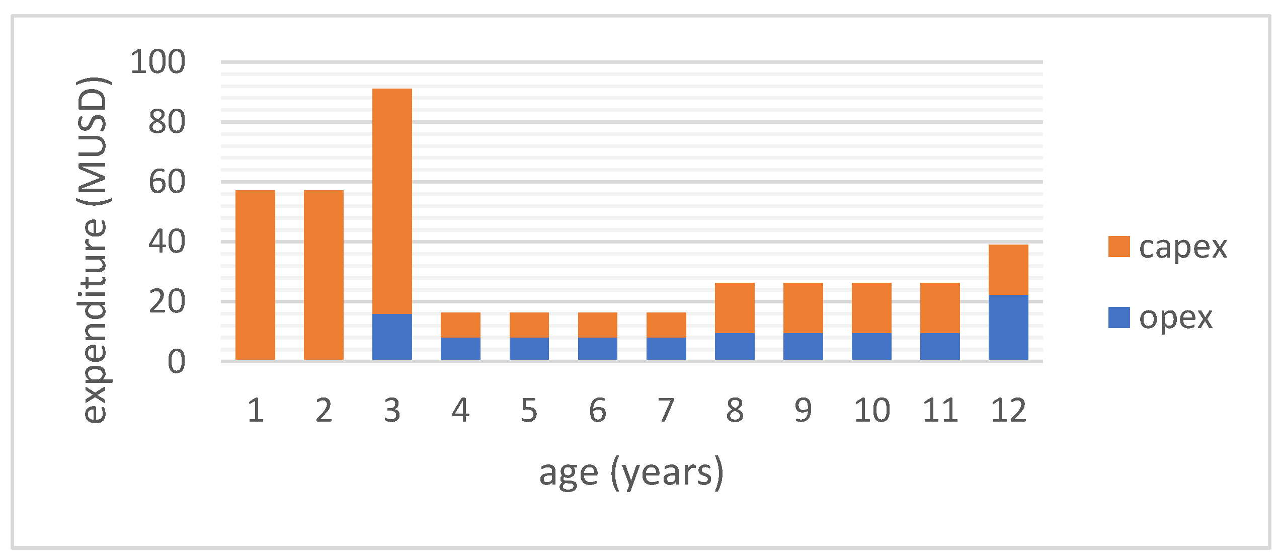
Figure 3.
Schematic of a standard production profile for a 4.5 BCM gas field. On plateau, the field produces about 6% of its estimated ultimate recovery (EUR) per year, before production enters a managed exponential decline of 11% per year. The field is decommissioned when its remaining net present value (NPV) drops to zero due to the decline in production.

Figure 4.
Breakdown of capital expenditure (capex) for individual field environments.
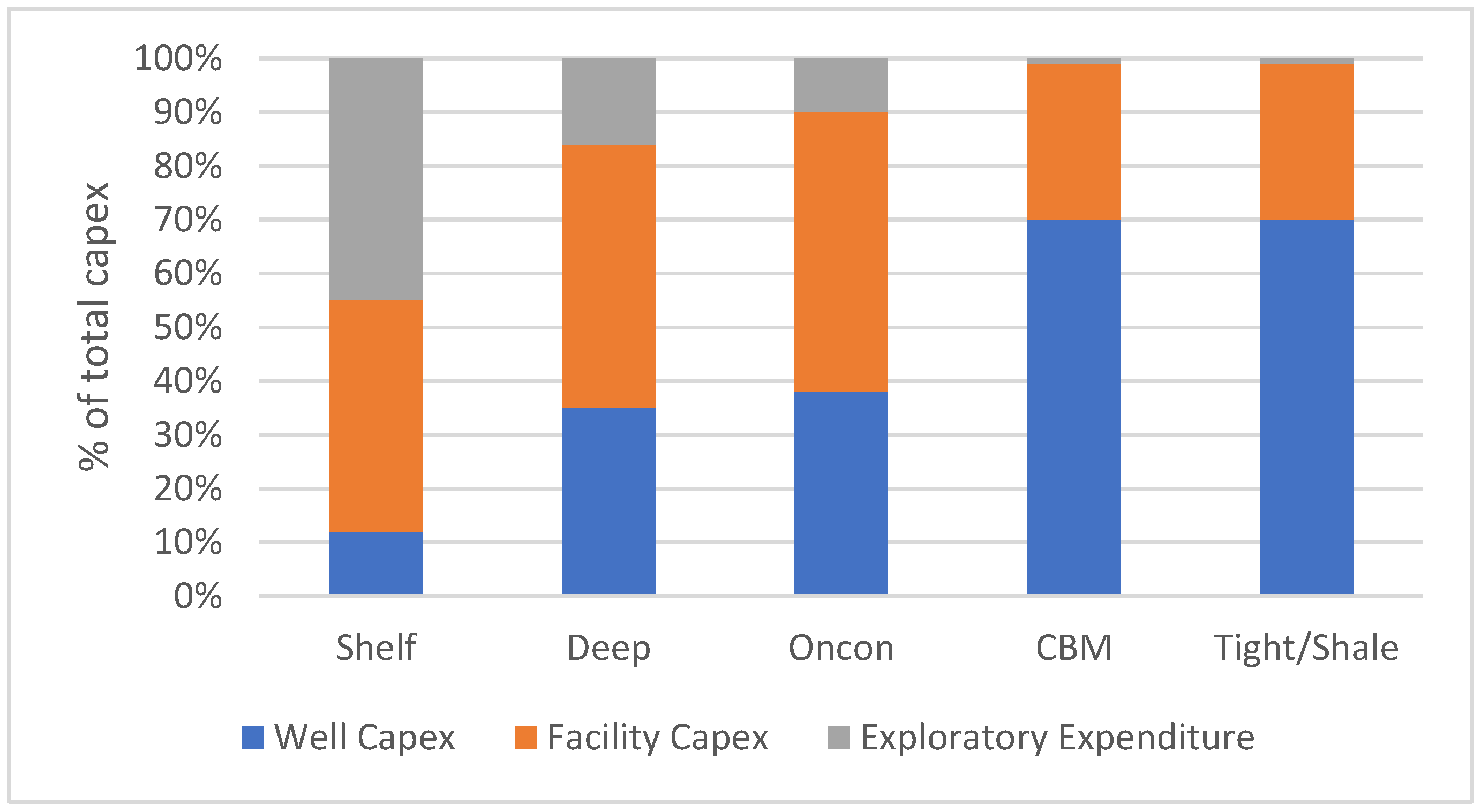
Figure 5.
Field size distributions showing the relative frequency vs. the log of the initial 2P EUR (in BCM) for (a) onshore conventional, (b) shelf, (c) deep offshore, (d) CBM, and (e) tight/shale. The bin width is 0.2. The number of fields used to derive the distributions is: tight/shale = 523, CBM = 29, onshore conventional = 241, shelf = 2534, deep offshore = 162.
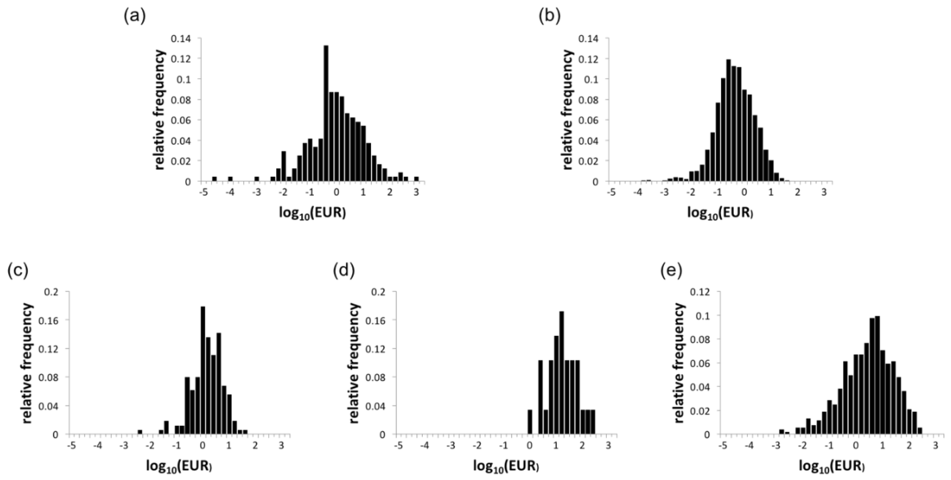
Figure 6.
Breakeven price as a function of production volume.
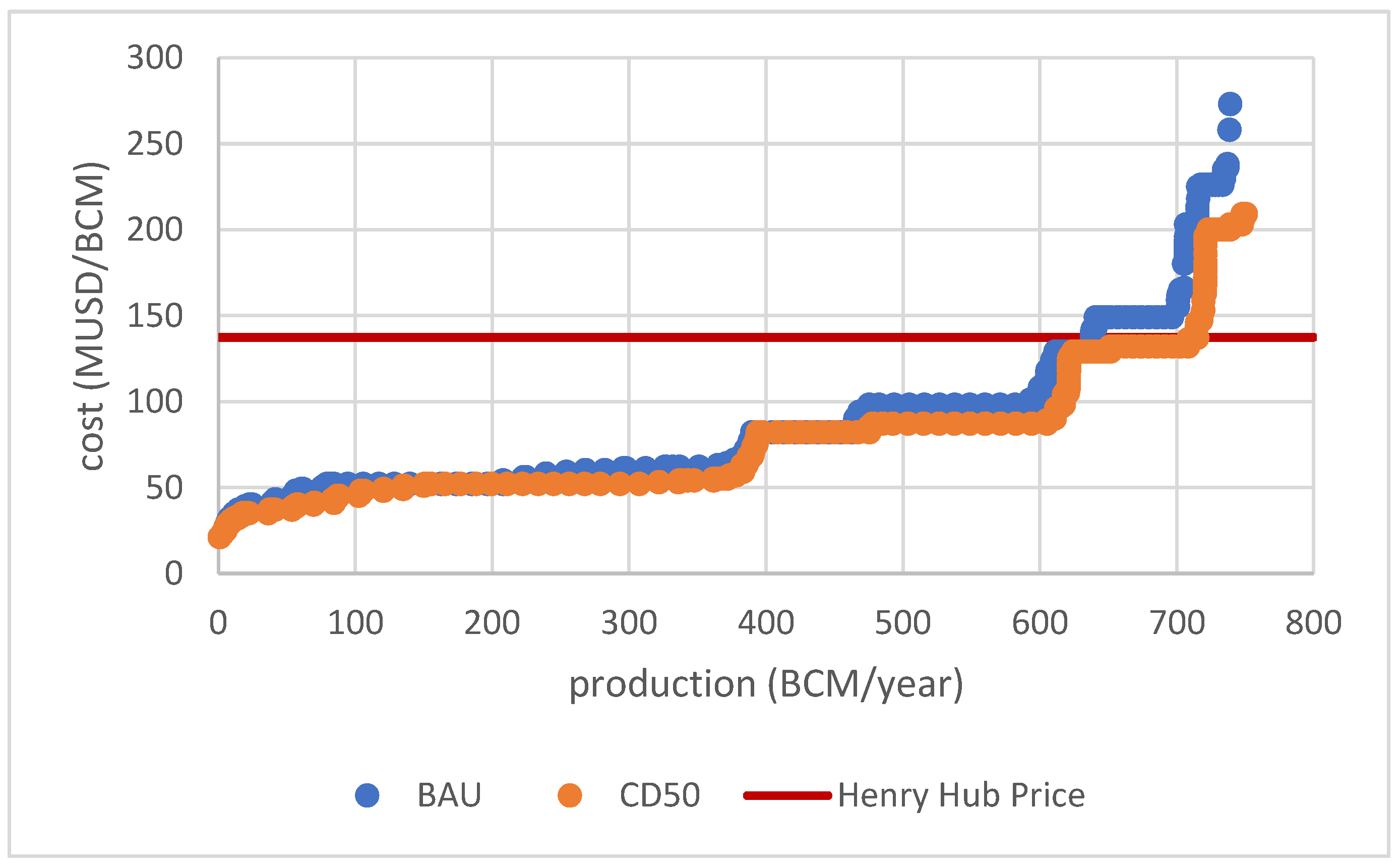
Figure 7.
Initial breakeven price as a function of well capex reduction.
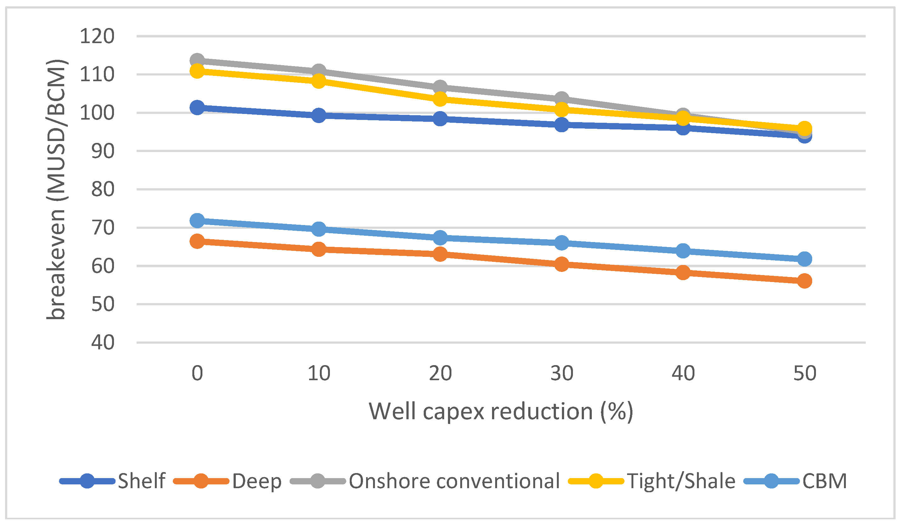
Figure 8.
Mid-plateau breakeven price as a function of well capex reduction.
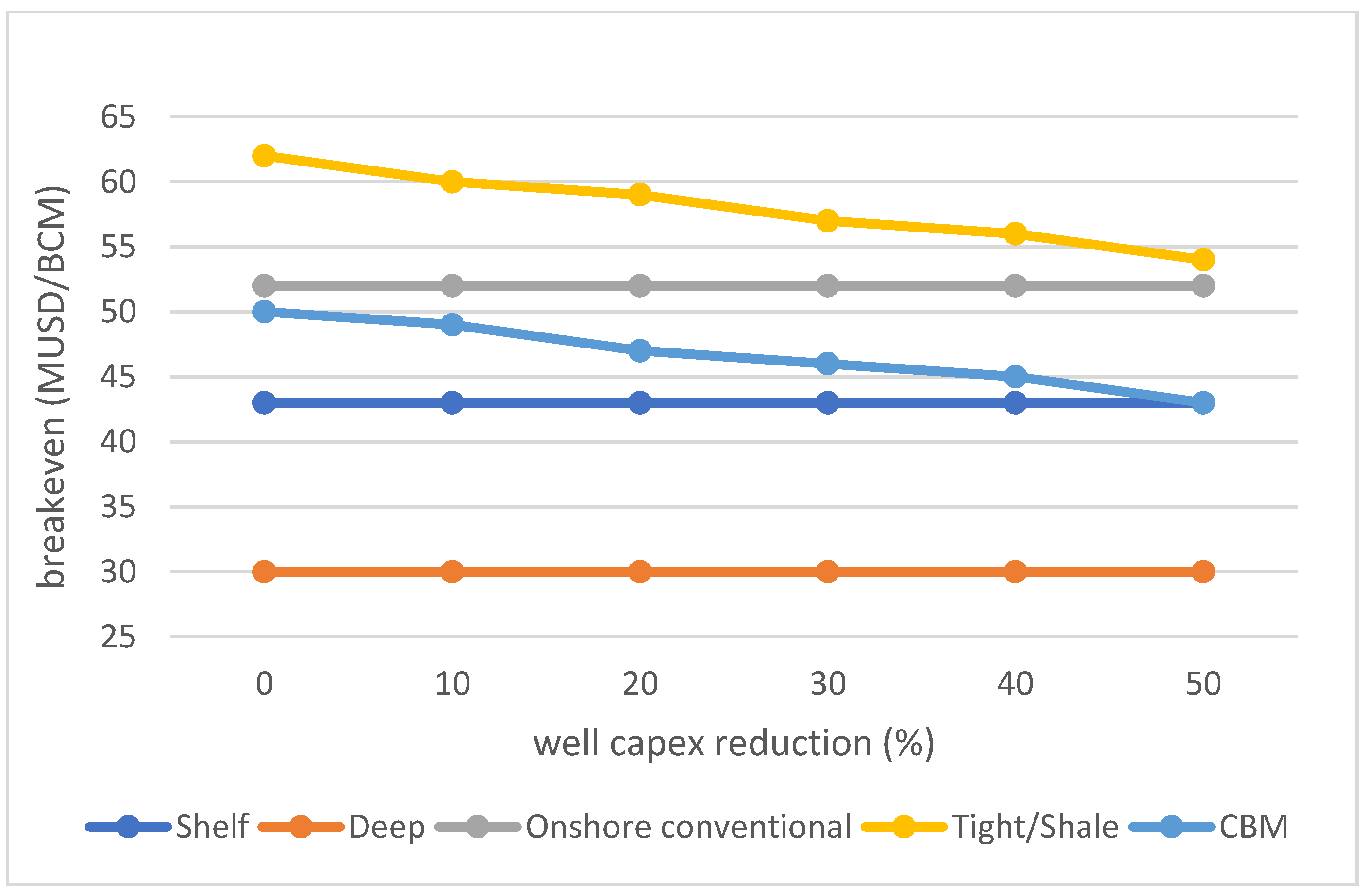
Figure 9.
Increase in NPV as a function of well capex reduction.
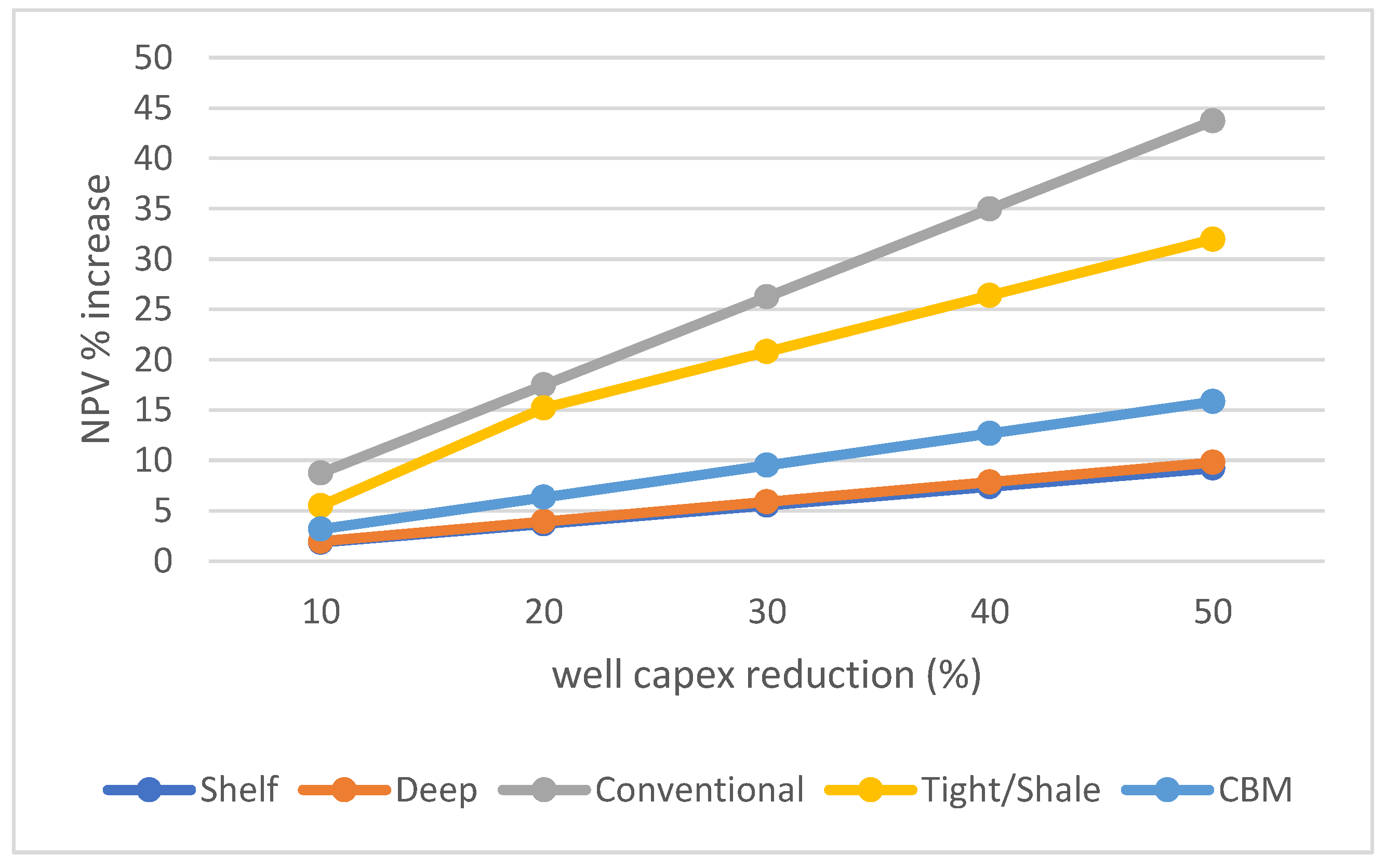
Figure 10.
Capital efficiency as a function of well capex reduction.
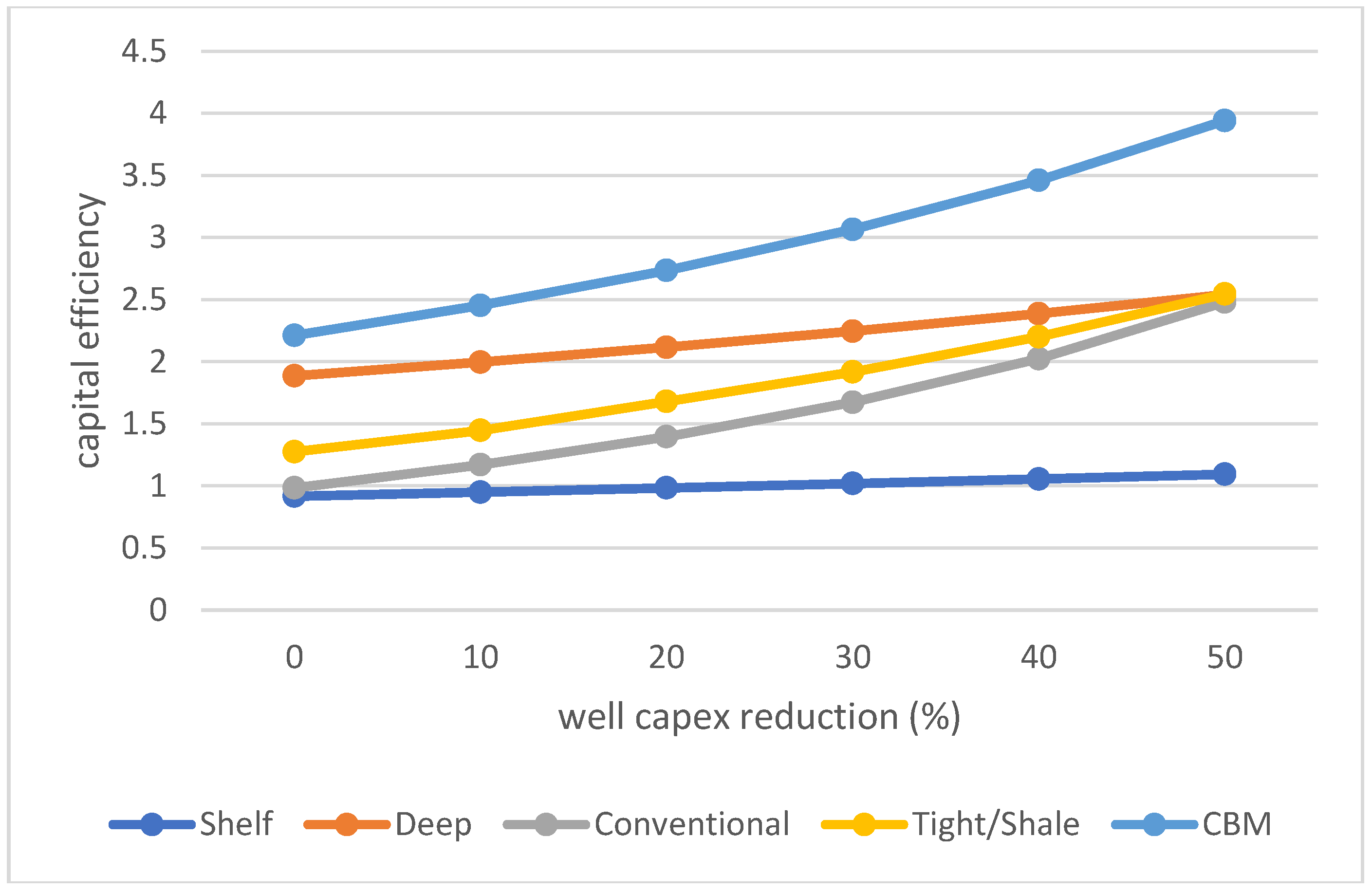
Figure 11.
Wellhead breakeven price as a function of cumulative 2P reserves held in producing fields in the US. For clarity, the breakeven is volume-weighted over all asset classes belonging to a given field environment. The business-as-usual scenario (full drilling costs) is shown in light shades and a CD50 scenario (representing a 50% reduction in drilling costs) is shown in dark shades. The CD50 scenario shows a reduction in breakeven prices across all field environments (the darker blocks are lower than the light blocks), as well as reserve additions in shale/tight and CBM field environments (the supply curve of darker blocks is shifted to the right).

Table 1.
Definitions of field environments.
| Field Environment | Definition | |
|---|---|---|
| 1 | Shelf | Offshore sandstone reservoirs in water depths <125 m |
| 2 | Deep offshore | Offshore sandstone reservoirs in water depths >125 m |
| 3 | Onshore conventional | Onshore sandstone reservoirs that do not rely upon hydraulic fracturing to achieve economically viable production rates |
| 4 | Tight/shale | Onshore sandstone and shale reservoirs that require horizontal wells with extensive hydraulic fracturing to achieve production rates that are economically viable |
| 5 | Coal bed methane (CBM) | Natural gas extracted from coal seams |
© 2018 by the authors. Licensee MDPI, Basel, Switzerland. This article is an open access article distributed under the terms and conditions of the Creative Commons Attribution (CC BY) license (http://creativecommons.org/licenses/by/4.0/).
Share and Cite
MDPI and ACS Style
Crow, D.J.G.; Anderson, K.; Hawkes, A.D.; Brandon, N. Impact of Drilling Costs on the US Gas Industry: Prospects for Automation. Energies 2018, 11, 2241. https://doi.org/10.3390/en11092241
AMA Style
Crow DJG, Anderson K, Hawkes AD, Brandon N. Impact of Drilling Costs on the US Gas Industry: Prospects for Automation. Energies. 2018; 11(9):2241. https://doi.org/10.3390/en11092241
Chicago/Turabian StyleCrow, Daniel J. G., Kris Anderson, Adam D. Hawkes, and Nigel Brandon. 2018. "Impact of Drilling Costs on the US Gas Industry: Prospects for Automation" Energies 11, no. 9: 2241. https://doi.org/10.3390/en11092241
Note that from the first issue of 2016, this journal uses article numbers instead of page numbers. See further details here.