Design and Experimental Implementation of a Hysteresis Algorithm to Optimize the Maximum Power Point Extracted from a Photovoltaic System

Abstract

In the several last years, numerous Maximum Power Point Tracking (MPPT) methods for photovoltaic (PV) systems have been proposed. An MPPT strategy is necessary to ensure the maximum power efficiency provided to the load from a PV module that is subject to external environmental perturbations such as radiance, temperature and partial shading. In this paper, a new MPPT technique is presented. Our approach has the novelty that it is a MPPT algorithm with a dynamic hysteresis model incorporated. One of the most cited Maximum Power Point Tracking methods is the Perturb and Observer algorithm since it is easily implemented. A comparison between the approach presented in this paper and the known Perturb and Observer method is evaluated. Moreover, a new PV-system platform was properly designed by employing low cost electronics, which may serve as an academical platform for further research and developments. This platform is used to show that the proposed algorithm is more efficient than the standard Perturb and Observer method.

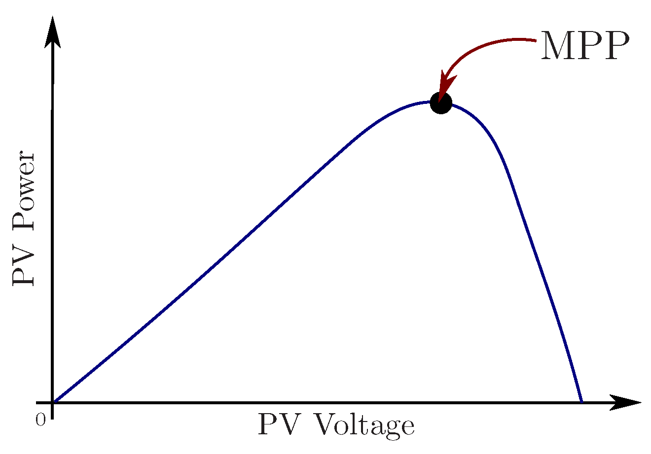
1. Introduction

Nowadays, the electrical energy extracted from green sources is considered an effective and necessary solution for today’s new development efforts since conventional energies (petroleum and natural gas) have had an enormous negative environmental impact on life on earth. Among the main available green resources (solar, wind, biomass, hydro and geothermal), sunlight is one of the most promising renewable energy sources due to it being estimated that the incidence of solar energy at the Earth’s surface is much greater than the world energy consumption [1]. In fact, if a PV system were developed by just covering only 0.1% of the Earth’s surface with an efficiency of 10%, it would suffice to satisfy our current energetic needs [2]. For instance, in the southeast of Spain, the current energy consumption of the greenhouses and the current CO${}_2$ emission produced by this sector would completely disappear if solar energy were used [3]. Moreover, solar energy is a unique available resource in the field of spacial solar system exploration, which is currently an important research topic. For these reasons, the use of solar energy has seen exponential growth in the last few decades. Furthermore, solar energy requires less maintenance, and it is implemented easier than other renewable energies [1]. However, the main disadvantage of photovoltaic systems is its low conversion efficiency of sunlight into electrical energy. Additionally, the proper energy storage provided by the solar panels is still an important challenge to deal with [4,5]. Hence, it becomes necessary to develop new techniques to extract, as well as possible, the maximum power from PV panels to achieve its maximum efficiency conversion.

Essentially, photovoltaic modules directly convert the sunlight into electric energy. The PV modules are traditionally made of several cells connected in series and in parallel arrangements. The type of connection depends on the voltage and current levels at which it is desired for the power system to work. The sunlight to energy conversion process requires only the use of semiconductors’ devices, where moving parts are not required, which is an important advantage with respect to, for instance, wind energy systems. Additionally, other positive characteristics of PV panels are related to its long effective life, high reliability, low maintenance-cost, and rapid response at its output [6].

In general, PV systems may be classified into three classes [7]: (1) the grid-connected configuration, (2) the stand-alone architecture, and (3) the hybrid systems. Most of the stand-alone PV systems have been employed to feed electrical power to isolation loads without access to the distribution lines [8]. Related to the grid-connected system, for instance, in 2014, the total installed PV modules in the main countries reached the capacity of 177 GW [9]. PV systems are able to accomplish oil energy independence and to encourage new economic and job opportunities [10]. For instance, the photovoltaic industry in the global market has achieved continuous growth since 2016 [11]. According to [12], these systems will soon become one of the main components of electrical power plants and smart grids. Many researchers are open to this topic, such as the development of new MPPT algorithms to PV system arrays operating under partial shading and exhibiting multiple local maximum power points [13,14], appropriate updating of the current grid coded [15,16], modeling and analysis of utility-scale photovoltaic units in hybrid energy storage devices [12], and so on [17,18,19]. Finally, the hybrid systems take advantage of the appropriate mixing combination between the grid-connected configuration and the stand-alone architecture. The approach presented in this paper is oriented to PV system stand-alone applications.

Ideally, under invariant irradiance conditions and fixed temperature, there is a unique operating point where the PV supplies its maximum power (see Figure 1). This is the maximum peak that can be found in the characteristic PV panel Power–Voltage curve and it is known as Maximum Power Point (MPP). The value of this Maximum Power Point depends on the current irradiance and the cell temperature and it is then necessary for an MPPT algorithm to ensure that the PV system operates with its maximum power conversion efficiency, or as close as possible, even when these conditions change. However, in real operating conditions, the influence of a temperature variation on the PV panel may be negligible compared to the irradiation changes [20,21]. In general, the MPPT is an important challenge because the condition that determines the amount of energy into the PV module may change at any time [22]. The principle of the MPPT requires a dynamical optimizator, which usually consists of a switching converter that is auto adjustable in terms of the voltage, current or power of the PV panel at its terminals. In consequence, the load seen by the panel is manipulated to achieve the MPPT objective [23,24].

Previously, numerous MPPT techniques have been proposed, developed and efficiently implemented [1,6,22,23,25,26,27,28,29,30,31,32,33,34]. Some of them are based on the PV model; for instance, those methods that fit in this branch are the Fractional Open-Circuit Voltage and Short-Circuit Current [24]. However, these techniques have the primary disadvantage of periodically requiring disconnection or realizing short-circuits in the PV module and then inducing a significant power loss [22]. On the other hand, the most simple methods are known by their easy implementation and control structure. Methods situated in this category are the Hill Climbing (HC) method [35], the Incremental Conductance (IndCond) technique [26] and the well known Perturb and Observer (P&O) algorithm [6,25,27,35]. Additionally, varied versions of conventional MPPTs, such as the modified version of the most popular techniques (HC, P&O, IndCond) have been developed to mitigate the drawbacks resulting from using the traditional algorithms [36,37]. Moreover, extremum seeking control techniques have also been implemented to realize the MPPT [20,21,30,38]. Finally, there are other control techniques that have been applied to extract the MPP from a PV cell by improving the behavior of classic techniques previously mentioned. For instance, some methods are based on artificial intelligence tools [39,40]. In this field, the most common are Artificial Neural Networks (ANNs), Genetic Algorithm (GA), Particle Swarm Optimization (PSO) and Fuzzy Logic Controller (FLC) [28,41]. A very deep discussion and a comparison of the different techniques have been studied in detail, for instance, in [1,6,7,24,27,29,30,35,42]. On the other hand, there exists a modified P&O algorithm with a fixed perturbation step that was developed to directly control the converter stage by eliminating the Proportional-Integral/hysteresis component from the main MPPT structure controller [7]. In contrast, some reports, for instance, the one presented in [8], employs a hysteresis strategy directly applied to the DC bus converter. Hence, if hysteresis is adequately implemented, it may be useful to increase the performance of a MPPT strategy. Based on the above discussed literature and for the best knowledge of the authors, there is no MPPT method that employs hysteresis directly in its algorithm. For this reason, the technique proposed here, which employs a dynamic hysteretic model as an MPPT algorithm, may be a novel technique in the PV panels’ field.

This paper presents two main objectives. The first one is to propose a novel MPPT approach. This suggested technique includes a dynamic hysteretic system, which is defined to evaluate the PV voltage and PV power to fulfill the MPPT aim. The second objective is to design and build a low cost PV-MPPT experimental evaluation platform to test new MPPT algorithms. The platform employs a motorized potentiometer that replaces the conventional DC/DC converter commonly used in many MPPT methods. In addition, the proposed hysteretic MPPT method is implemented in this platform to evaluate its performance. A well-known P&O algorithm is also implemented to have a comparison between both methods.

The rest of this paper is organized as follows. Section 2 gives the PV modeling, and Section 3 presents an equivalent model of the typical DC/DC converters used in MPPT methods. Section 4 describes the usual Perturb and Observer algorithm. In Section 5, the proposed MPPT approach is presented. Section 6 describes our experimental platform design. Section 7 gives the experimental results and discussions. Finally, conclusions are stated in Section 8.

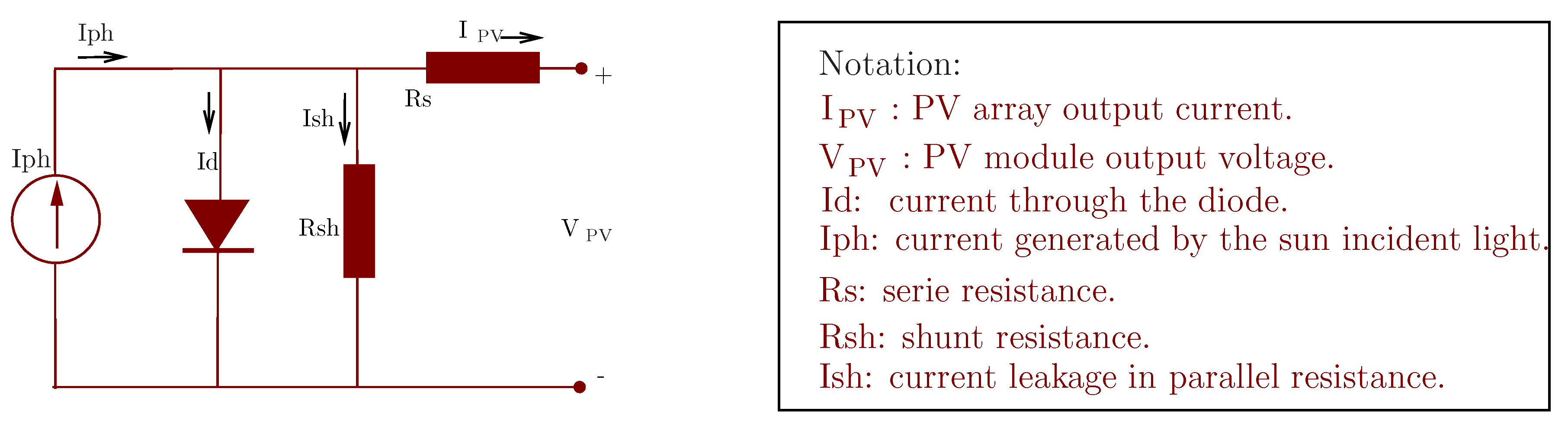
2. Photovoltaic Modeling

The PV modeling has been a remarkable topic in the solar energy area since some MPPT methods are based on the knowledge of the PV model [1,24,25]. Some other MPPT techniques do not require the PV model, as is the case of the algorithm proposed in this paper. However, it is necessary to have a basic knowledge of the PV panel operation. For this reason, a simple based current model is presented next.

The most common PV panel models basically consist of series and parallel resistors connected to a single diode. This can be seen as a current source in parallel with a diode, a shunt resistance $R_{sh}$ and a serial resistance $R_s$ as shown in Figure 2. The serial resistance mainly affects the slope of the Current–Voltage (I–V) characteristic curve at the high voltage levels approaching the open-circuit voltage. On the other hand, the shunt resistance affects the I–V curve slope at current levels close to the short-circuit current [24]. Additionally, the diode takes into account the physical effects at the silicon P-N junction of the PV cell. Finally, the current source generator corresponds to the photo-induced current that depends on the semiconductor’s characteristics. From Figure 2, the equation of the PV output current ($I_{PV}$) of the solar cell yields:

$$I_{PV}=I_{ph}-I_d-I_{sh},$$

(1)

where $I_{ph}$, $I_d$ and $I_{sh}$ are described in the notation given in Figure 2. Furthermore, $I_d$ is given by [24]:

$$I_d=I_0·(e^{q\frac{(V+I{R}_s)}{nKT}}-1),$$

(2)

where $I_0$ is the saturation current, q represents the electron charge, and K is the Bolzman constant. Moreover, n is the diode factor and T is the temperature on the P-N junction of the diode. The current $I_{ph}$ can be expressed as follows [24]:

$$I_{ph}=\frac{G}{Gstc}·(I_{sc,ref}+{\mu }_{sc}(T-T_{stc})),$$

(3)

where ${\mu }_{sc}$ is the temperature coefficient of the short circuit current, G is the irradiation effect, $G_{stc}$ is the irradiation effect in specific operating conditions (defined as standard conditions [24]), and $I_{sc,ref}$ is the short circuit current at a given reference temperature. On the other hand, the saturation current is given by:

$$I_0=C·T^3·e^{(-\frac{E_{gap}}{kT})},$$

(4)

where $E_{gap}$ is the band gap of the semiconductor material and C is the temperature coefficient [24]. Therefore, the PV current can be rewritten as:

$$I_{PV}=I_{ph}-I_0·[e^{q\frac{(V+I{R}_s)}{nKT}}-1]-\frac{V+R_s{I}_{PV}}{R_{sh}}.$$

(5)

The model shown in Figure 2 is the representation for a single PV cell. A set of single PV cells can be connected in a serial/parallel arrangement in order to be used as a PV module that can also be named as a panel, string or a whole PV field.

3. An Equivalent Model of the DC/DC Converter in PV-MPPT Systems

In order to achieve the maximum power point tracking in PV systems, it is necessary an electronic conversion stage between the PV module and the load that will acquire the electrical power produced by the PV panel. This intermediate stage must be able to manipulate its output in accordance with the changes in PV voltage and current, which are sensitive to irradiance and temperature variations. By monitoring these changes, a parameter in the converter must be adjusted to satisfy the MPPT objective. Usually, this conversion stage is realized by a DC/DC converter that manipulates its output through the control law generated by the MPPT algorithm. The common block diagram of a MPPT in PV systems is depicted in Figure 3a.

The external load of the PV panel is imposed onto it, and then the DC/DC converter drives the current to the load according to the MPPT objective. In other words, the converter is used to perform impedance matching [20]. This means that the duty cycle of the converter has a direct effect in the load seen by the PV panel when the load is connected to the output of the converter. The scheme in Figure 3b realizes the same task as the common structure; however, it is more simple to implement. Hence, the diagram in Figure 3b, which employs a manipulable potentiometer, emulates the system in Figure 3a.

The most common DC/DC converters used in a PV panel area are the Boost converter and the Buck converter. Both converters accomplish the objective to adjust the equivalent impedance seen by the PV module at its terminals by using the relation between the PV module and the load voltage [20,23,24].

Based on the scheme shown in Figure 3b, this paper develops an MPPT implementation by controlling a DC motor mechanically connected to a potentiometer. The potentiometer terminals are connected to the PV panel terminal connections. In this way, the load, $rl$, seen by the PV panel is automatically actuated to the track as well as possible, the maximum power point (see Figure 3b) [20]. The control signal acquired by the DC motor will be generated by the instrumentation stage of the signal produced by the MPPT algorithm.

Regarding how to tune the output resistance $rl$ related to a specific application (see Figure 3), it can be realized, for instance, by using the equivalent resistance formula. For example, in Buck DC-DC converters, it is well known that [32]:

$$rl=\frac{\eta Rl}{D^2},$$

where $\eta$ is the converter efficiency, D is the converter duty cycle and $Rl$ is the load of the original application. For more options to calculate the equivalent resistance according to a given application, see [43].

In summary, in contrast with the typical DC/DC converter used in MPPT implementations, the MPPT control objective in this paper is to properly manipulate the load via the DC motor, such that the available maximum electrical power of the PV panel can be transferred to the load, as close as possible.

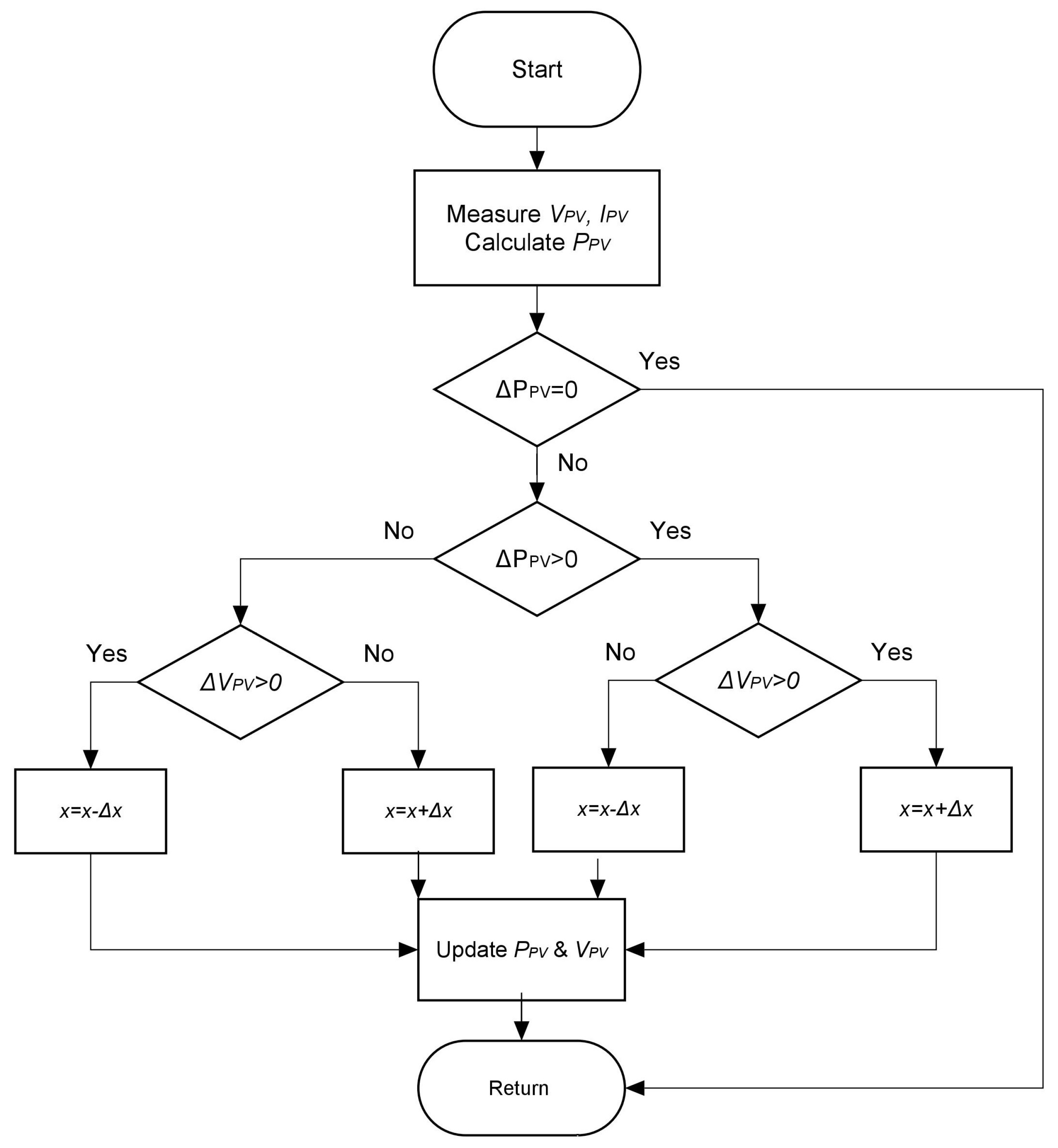
4. The MPPT Perturb and Observer Method

Among all MPPT techniques, the P&O algorithm is one of the most popular techniques. Actually, its first use goes back to the 1970s [24,44]. The Perturb and Observer algorithm is essentially based on continuously monitoring the voltage and current of the PV panel to estimate its output power. Hence, the variation in PV voltage ($\Delta V_{PV}$) and PV power ($\Delta P_{PV}$) are used by the algorithm and it produces a controlled perturbation command (the reference command) to change the PV operation point [29]. Lately, the maximum power point is achieved by adequately adjusting the perturbation. This algorithm is described as follows [6,29,31]:

• If both the power and voltage increase ($\Delta P_{PV}>0$ and $\Delta V_{PV}>0$), it means that the operating point has been moved forward and the search of the MPP continues in the same direction.
• On the other hand, if power decreases and voltage decreases ($\Delta P_{PV}<0$ and $\Delta V_{PV}<0$), it indicates that the MPP search is oriented in the wrong direction.
• The third possible case is when the power increases ($\Delta P_{PV}>0$), but the voltage decreases ($\Delta V_{PV}<0$). This indicates that the search of the MPP is oriented in the right direction.
• Finally, the last possible situation is presented when the power decreases ($\Delta P_{PV}<0$) and the voltage increases ($\Delta V_{PV}>0$). This case indicates that the MPP search is incorrectly oriented.

According to the four possible scenarios above, the MPPT P&O algorithm redefines the state of the controlled perturbation and manipulates the load seen by the PV panel at its terminal connections through the conversion stage. This algorithm can be captured through the following discrete-time dynamic model (for more details see [24]):

$$x(k+1)=x\left(k\right)+(V_{PV}\left(k\right)-V_{PV}(k-1))·\mathrm{sgn}(P_{PV}\left(k\right)-P_{PV}(k-1)),$$

(6)

where sgn is the signum function and $x\left(k\right)$ represents an internal "perturbation" variable and it may be further processed to generate the required MPPT control signal. This perturbation signal could be a Pulse Width Modulation (PWM) duty cycle depending on the P&O implementation. The time perturbation period is established according to the digital device in solving the above discrete-time system. Finally, Figure 4 shows the classical flowchart of the standard P&O algorithm [6,35,42].

To conclude, the P&O method is an algorithm of low complexity and is easy to implement [6]. However, due to its nature of constantly perturbation, when the MPP is closely reached, the PV output power oscillates around its maximum power point. It implies important power loss in the PV system [29].

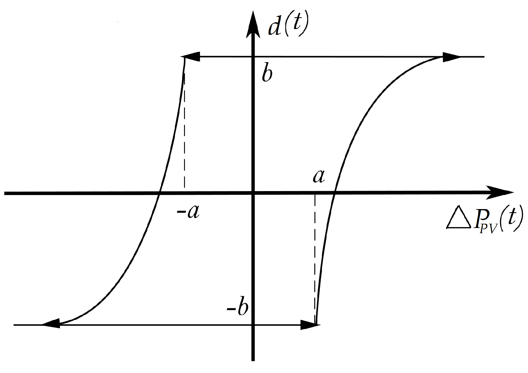
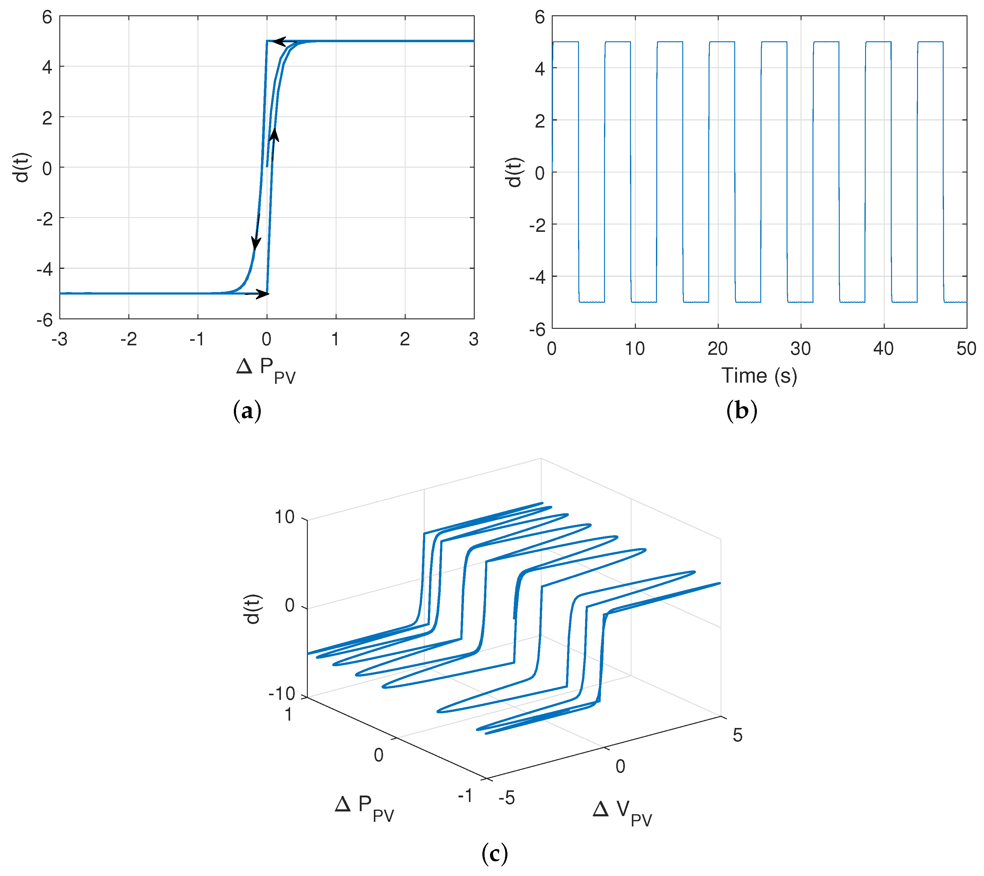
5. The Proposed MPPT Algorithm by Using a Dynamic Hysteresis Model

This approach incorporates a dynamic hysteresis model, which employs information from PV voltage and PV current and then calculates the PV power, in the same framework as the Perturb and Observer method. Our design essentially uses the PV power and PV voltage as inputs to a dynamic hysteretic system. In this way, an adequate reference command signal is generated to optimize the tracking of the maximum power point. It is well known that the hysteresis behavior can be recognized as a system with memory, exhibiting dependence of the current state on its past history [45]. Hence, hysteresis adjusts its output depending on the past state of its internal variable and its inputs. Precisely, our design takes advantage of this main property.

The proposed hysteresis model as a MPPT algorithm arises from the use of a signum function as a representation of a memory action or memory device, as in previous works by the authors [45,46,47]. Just as the P&O algorithm uses signum function to evaluate the direction of the voltage and power (see Equation (6)), the proposed hysteresis MPPT algorithm employs this function, but with the contrasting difference that, in our approach, the past voltage and current are taken into account. In this manner, our hysteresis based MPPT algorithm is:

$$\dot{d}\left(t\right)=\alpha [-d\left(t\right)+b\mathrm{sgn}(\Delta V_{PV}+a\mathrm{sgn}(\Delta P_{PV})],$$

(7)

where a and b $\in R^{+}$ are the hysteresis loop parameters and $d\left(t\right)$ is the internal variable of the model. For instance, Figure 5 shows a characteristic hysteresis behavior by varying $\Delta P_{PV}$ and keeping constant $\Delta V_{PV}$ with respect to $d\left(t\right)$. In Equation (7), the transition time-rate between b and $-b$ is governed by the real positive parameter $\alpha$. Hence, these parameters can be properly adjusted in order to set the response time or the hysteresis width. Actually, in our design, $\Delta V_{PV}$ and $\Delta P_{PV}$ are invoked as the inputs to the hysteresis system. Then, $\Delta P_{PV}$ and $\Delta V_{PV}$ collaborate jointly to drive the hysteresis loop behavior to fulfill the MPPT objective. Therefore, Equation (7) is presented as a new MPPT technique where the output $d\left(t\right)$ is directly used as the MPPT reference command signal.

To illustrate and validate the hysteresis behavior of system Equation (7), consider the following scenario: $\Delta P_{PV}=\sin \left(0.1t\right)$, $\Delta V_{PV}=5\sin \left(t\right)$, $a=1$, $b=5$ and $\alpha =50$. The obtained hysteretic loop $d\left(t\right)$ vs. $\Delta P_{PV}$ is shown in Figure 6a. On the other hand, the hysteresis loop in three dimensions is depicted in Figure 6c and the time response of the variable $d\left(t\right)$ is reproduced in Figure 6b. This figure represents a train of pulses that will be adapted to be the MPPT reference command signal. Naturally, in the implementation, since the PV panel is sensitive to environment changes, the width pulse will change depending on the changes in voltage and current. In this way, the PV maximum power point tracking will be, as close as possible, achieved.

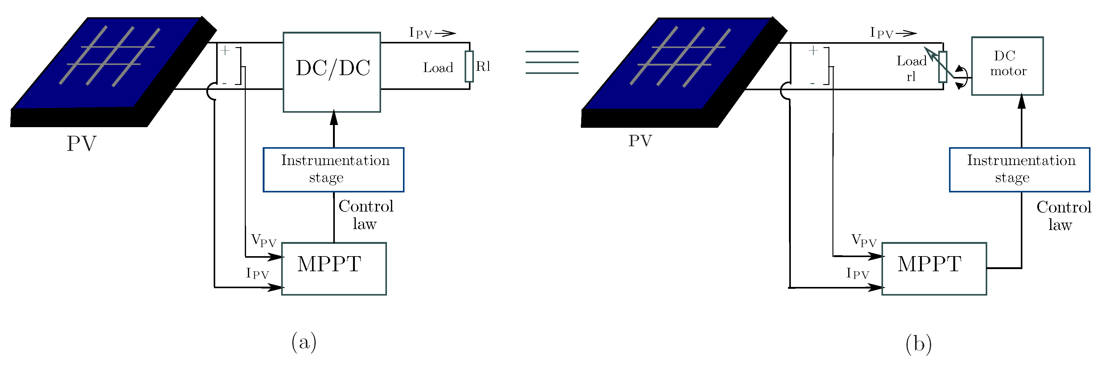
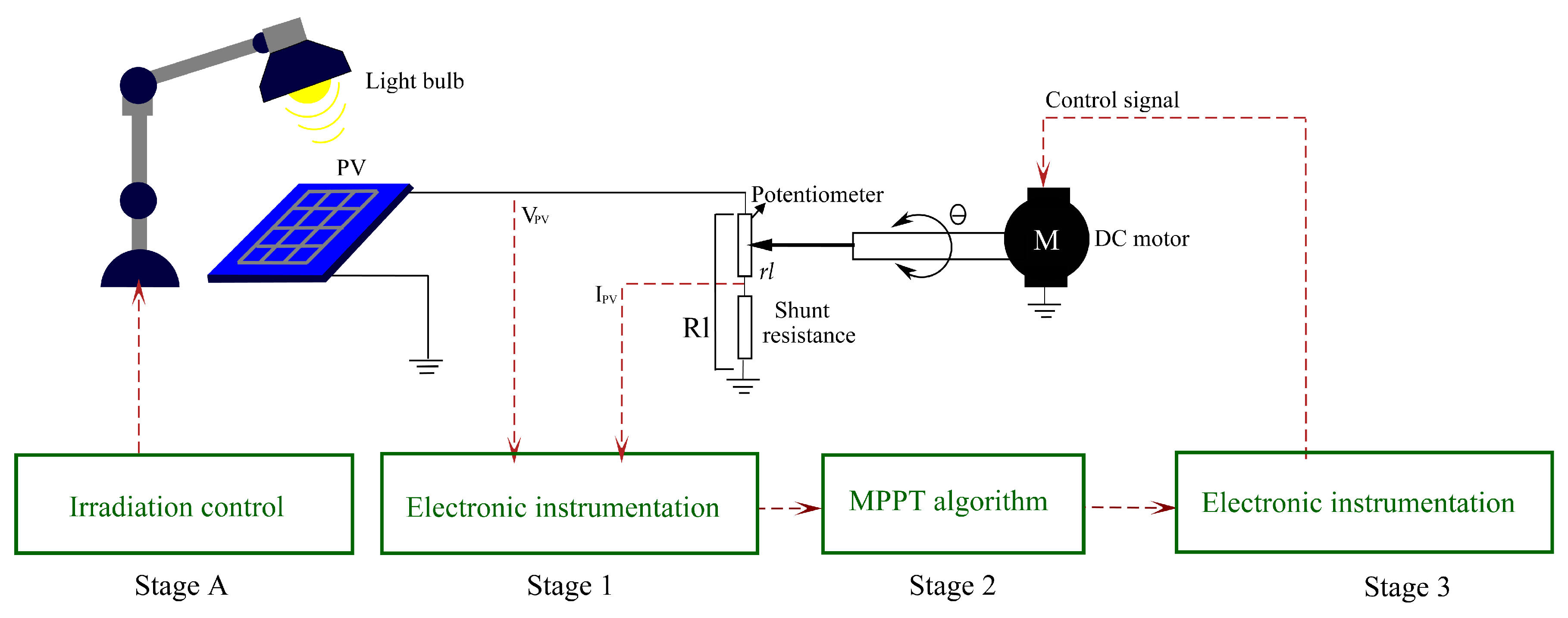
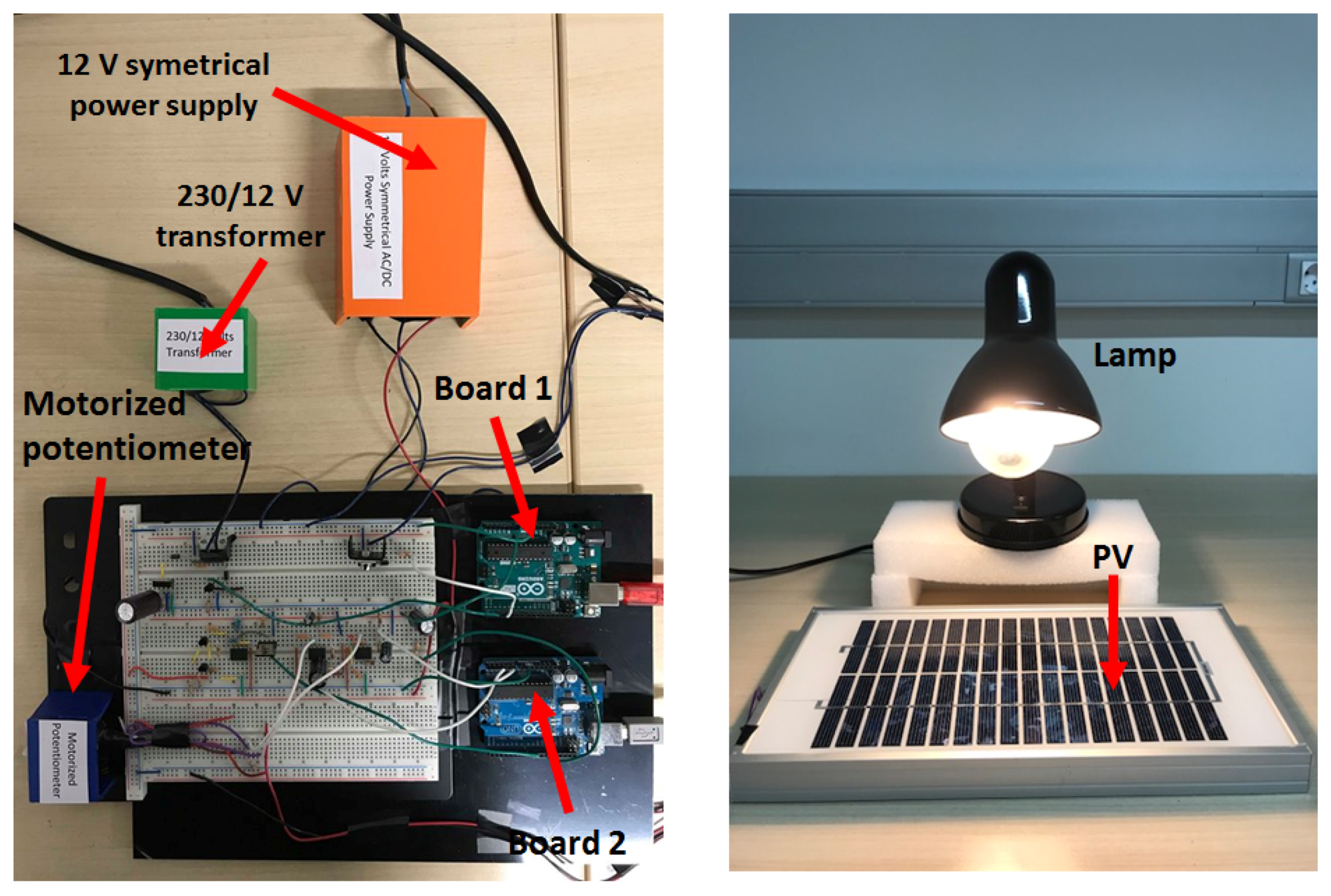
6. A PV-MPPT Experimental Platform

This section presents our designed platform set up in CoDAlab (Control, Dynamics and Aplications laboratory, Mathematics Department, Universitat Politècnica de Catalunya-UPC, https://codalab.upc.edu/en), where the two MPPT algorithms described in previous sections are implemented and validated. An overview of this platform is depicted in Figure 7. This is constituted by the following devices:

• A 5 W photovoltaic module Intertek IP65-IEC61215 (Intertek, London, UK) supplying a maximum voltage in close-circuit of 17 V and 21 V in open-circuit.
• An Arduino Uno board (labeled here as Board 1) to automatically control the intensity light of the bulb.
• A lamp with a 100 W bulb to emulate the irradiation variation and shading conditions.
• A 22 $\Omega$ shunt resistance used to instrument the supplied PV current to the load.
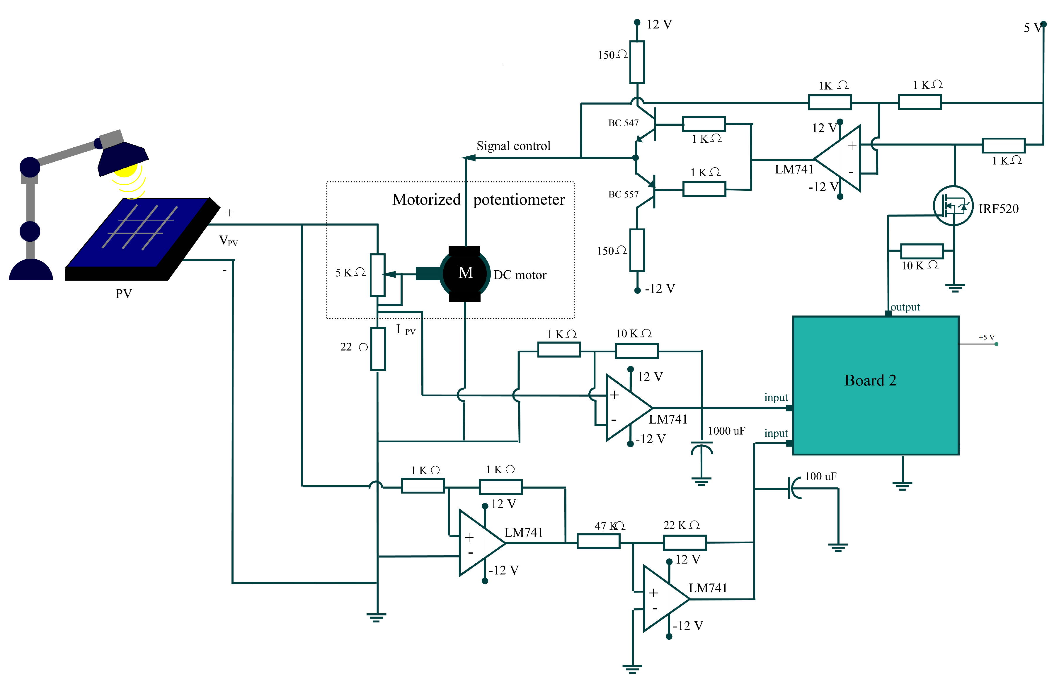
• A motorized-potentiometer constituted by a DC motor mechanically linked to a 5 k$\Omega$ potentiometer. This potentiometer emulates the load seen by the PV panel.
• A second Arduino Uno board (labeled here as Board 2) where the MPPT control algorithm is implemented.
• An electronic instrumentation development to couple the inputs and output signals to/from Board 2.

6.1. Technical Specifications

Some necessary technical specifications to properly realize the MPPT experiments are explained next. These specifications are divided into four stages labeled as depicted in Figure 7:

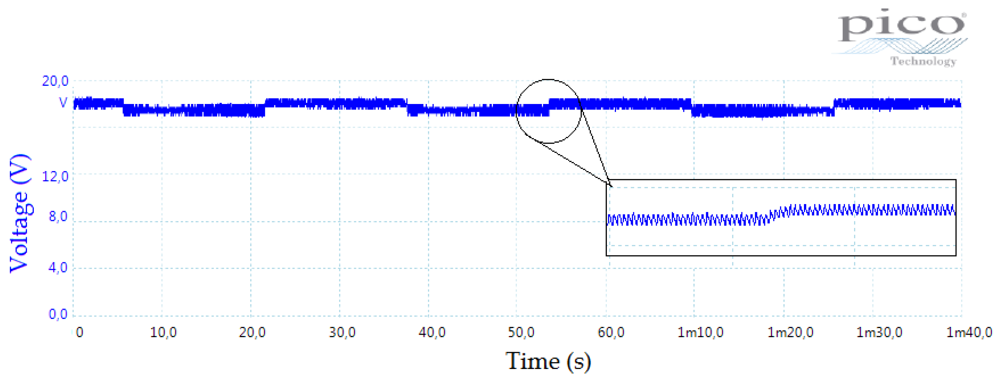
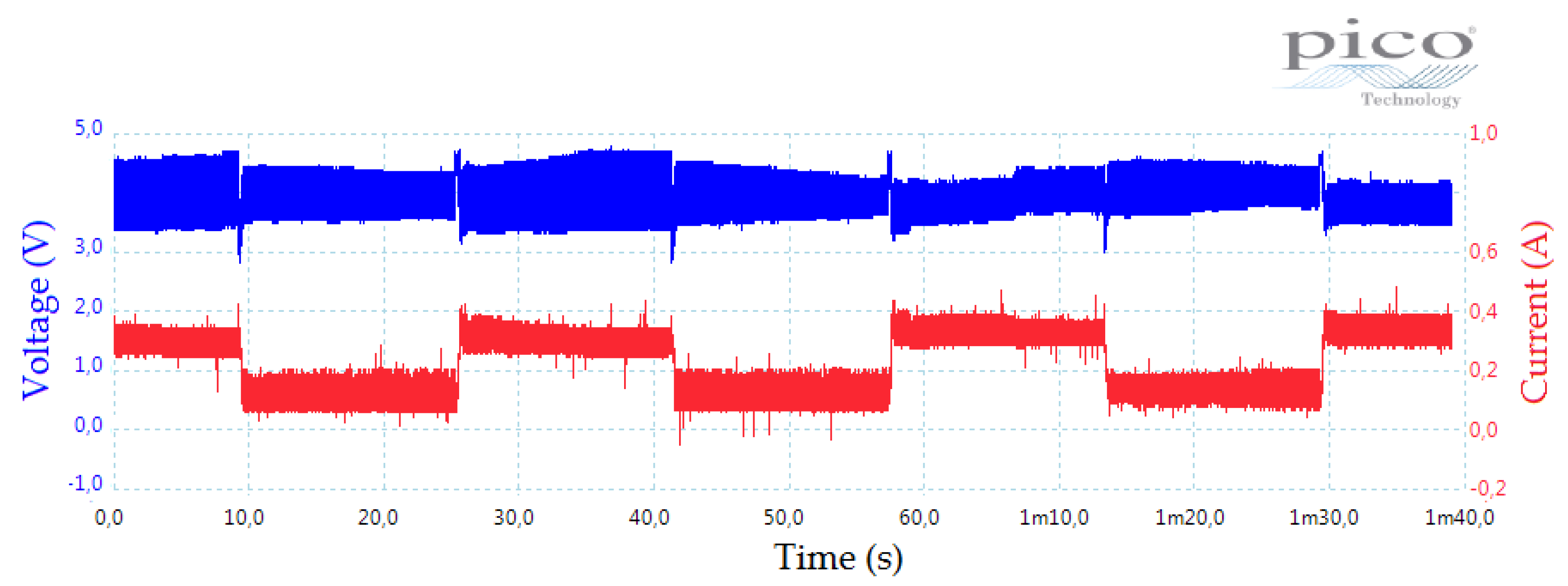
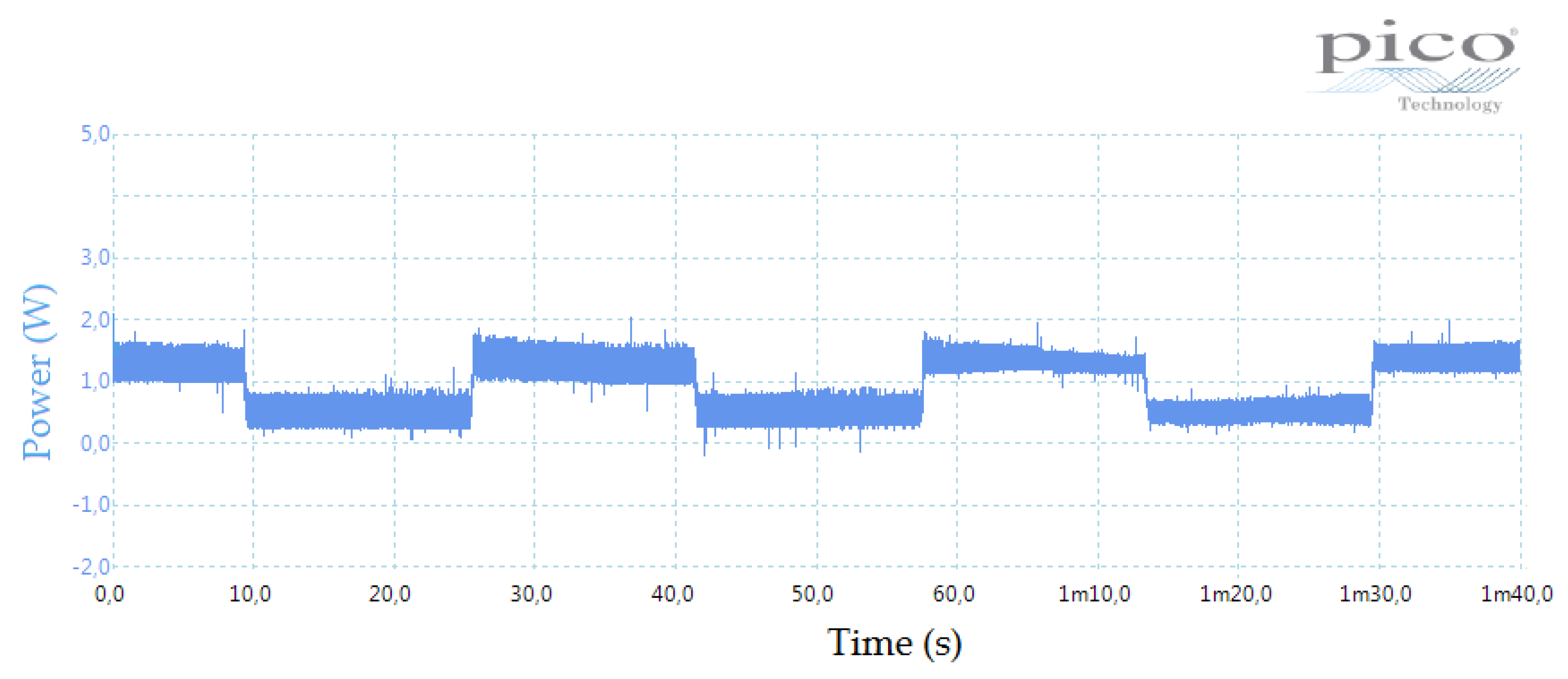
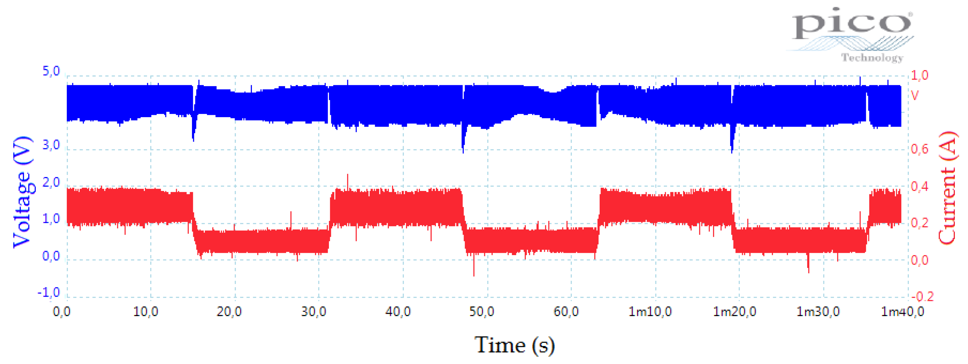
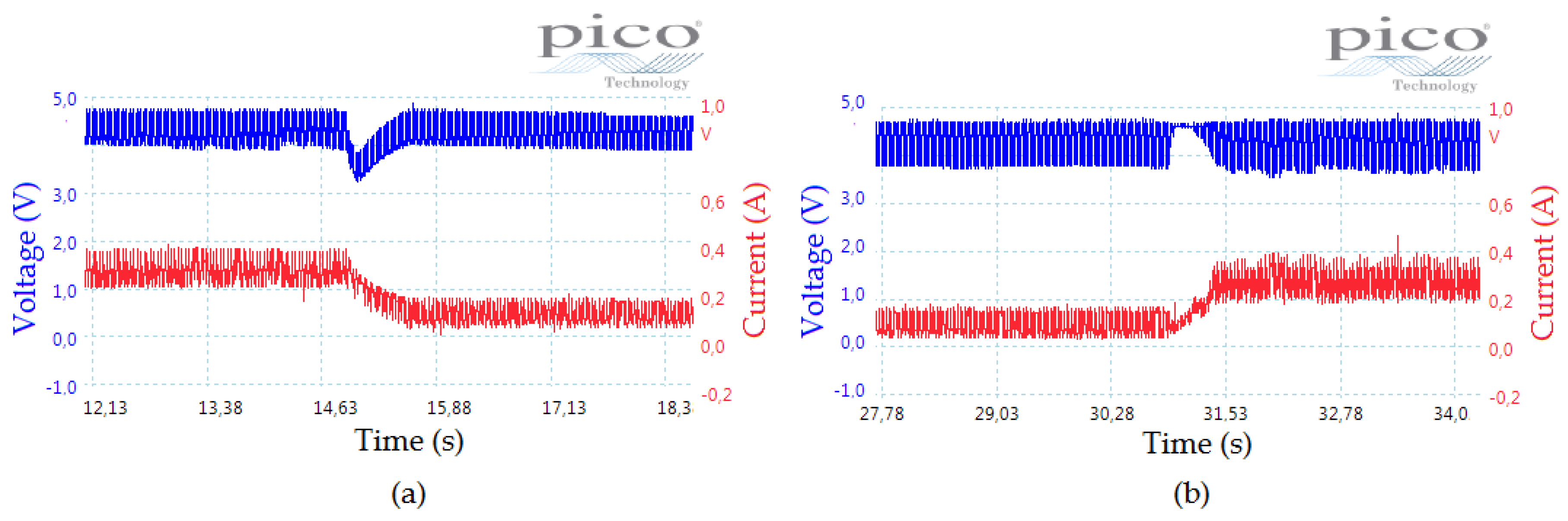
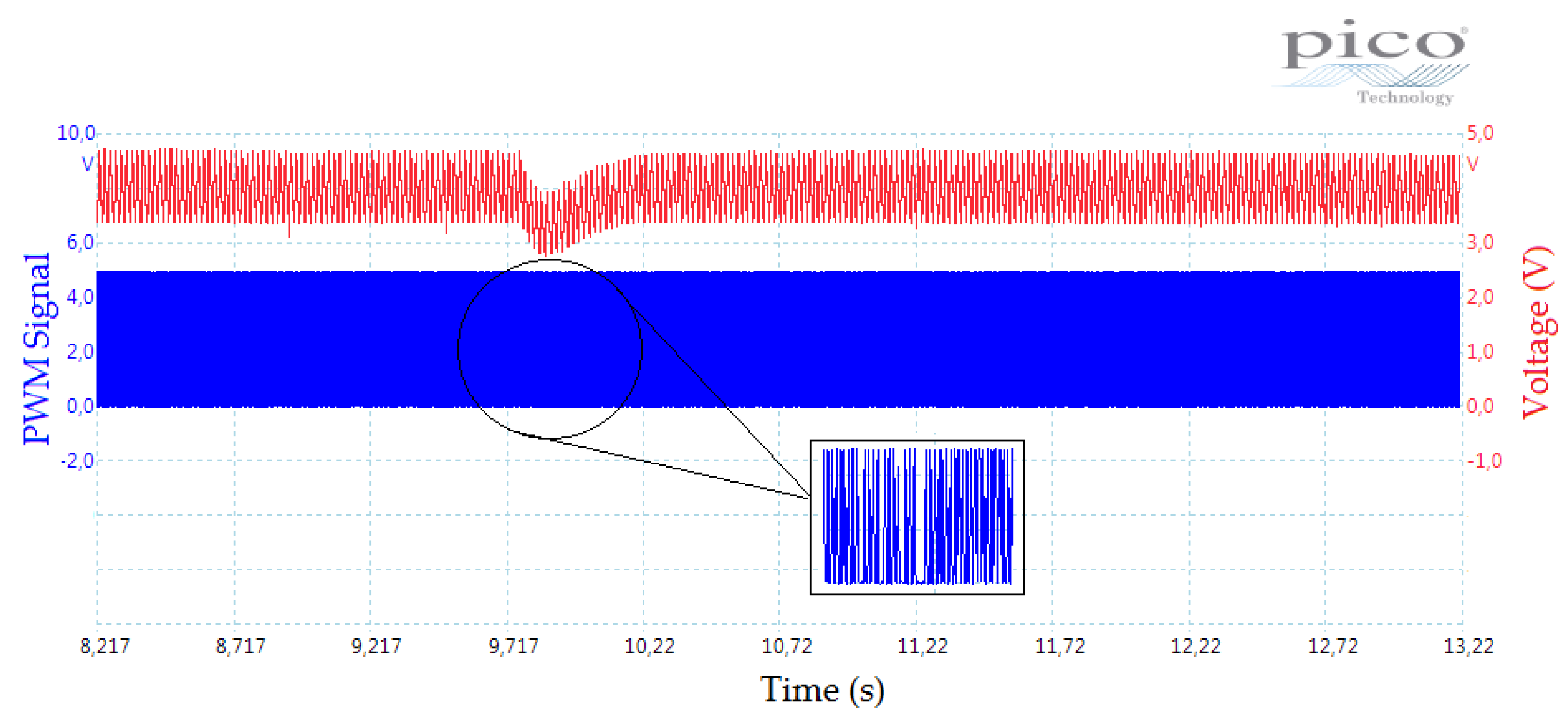
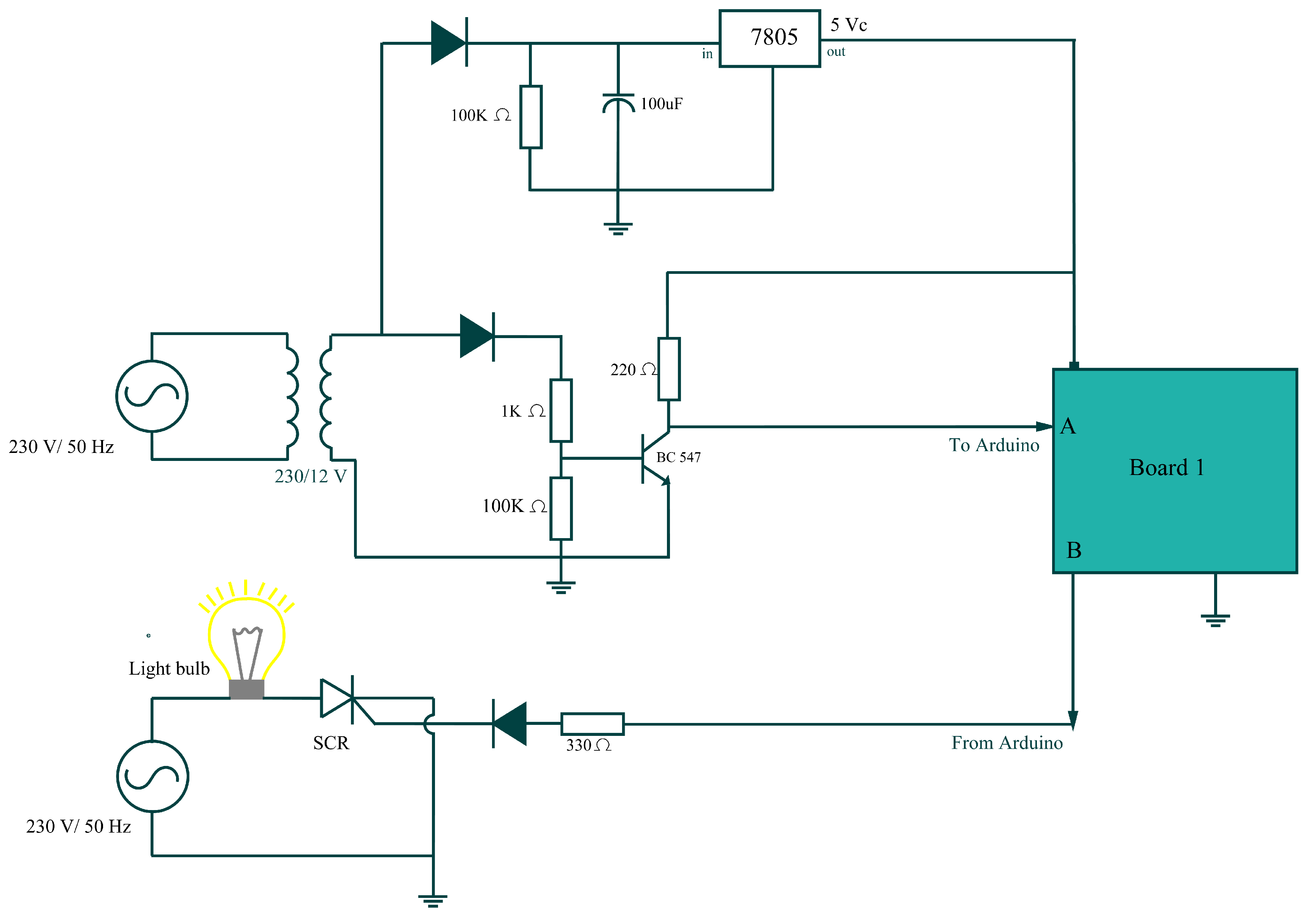
• Stage A: The irradiation control stage consists of Board 1 and an electronic instrumentation system. The general electronic circuit of this stage is presented in Appendix B, Figure A1. In this stage, an intentionally repetitive blinking light phenomenon was induced. Because of a PV panel being too sensitive to this kind of light perturbation, our experiment platform is able to emulate, for instance, a fast shading light condition [25,48]. Specifically, for the experiments shown in this paper, two levels of light intensity were programmed. The PV voltage in open-circuit under the effect of the irradiation changes is shown in Figure 8. Here, the automatic change of these two light intensity levels is made evident. In addition, the effect induced by the blinking phenomenon in the light bulb is clearly perceived. Note that this stage is independently designed from the other stages that integrate our PV-MPPT system.
• Stage 1: This stage consists of an electronic circuit, shown in Appendix B, Figure A2, which allows the PV voltage and PV current signals to be readable by the Arduino (Board 2). This is because the Arduino board reads voltages in the range of 0–5 V and our PV panel can produce up to 17 V.
• Stage 2: This stage involves the Arduino Uno (Board 2) where the MPPT algorithms are coded. The programed codes for experimental implementation are presented in Appendix C. Both algorithms, the P&O method and our hysteresis approach, generate a reference command signal (named here $X:=X\left(t\right)$), which assists with accomplishing the maximum power point tracking. Moreover, in this stage, a classic controller was implemented to stabilize the DC motor [20]. In this case, a proportional-controller (P-controller) that stabilizes the position of the motor around a set point value is employed. Thus, the P-controller was developed in terms of the position of the motor ($\theta$) captured by the potentiometer (see Figure 7). Since the position of the motor is directly related to the resistance of the potentiometer, the P-controller is obtained from the voltage point of view:

  $$V_{PV}=R_l·I_{PV};R_l:=R_l\left(\theta \right).$$

  (8)
  Therefore, our P-controller is expressed as: $u=k_p·(V_{PV}-V_{sp})$, where $k_p$ is the proportional gain and $V_{sp}$ is the set point established by the user. The P-controller coupled to the reference command signal (X) obtained from the MPPT algorithm can then be captured in the following control law (From the closed-loop system stability point of view, it is well known that a DC motor is controllable by a proportional controller):

  $$u_T=k_p·(V_{PV}-V_{sp}+X).$$

  (9)
  Since the Arduino analog outputs employ a PWM format according to the instrumentation stage, the above control law requires being translated into a PWM signal by using the Arduino instruction analogWrite (version 1.8.5-Windows, Arduino, Turin, Italy). Hence, the Equation (9) is rewritten as follows:

  $$u_{PWM}=k_p·(V_{PV}-V_{sp}+X)+V_{offset},$$

  (10)

  where $V_{offset}$ is selected here as the medium value of the Arduino PWM duty cycle range (255/2) since the DC motor must turn both left and right. On the other hand, $u_{PWM}$ is actually the duty cycle used by Arduino to generate the PWM output signal. Then, this signal will drive the DC motor through the electronic stage. In consequence, Equation (10) has the following objectives:

  – 

  to stabilize the motor around the $V_{sp}$ value through the P-controller,

  – 

  to navigate the DC motor position by following the MPPT reference command signal X from the $V_{sp}$ reference.

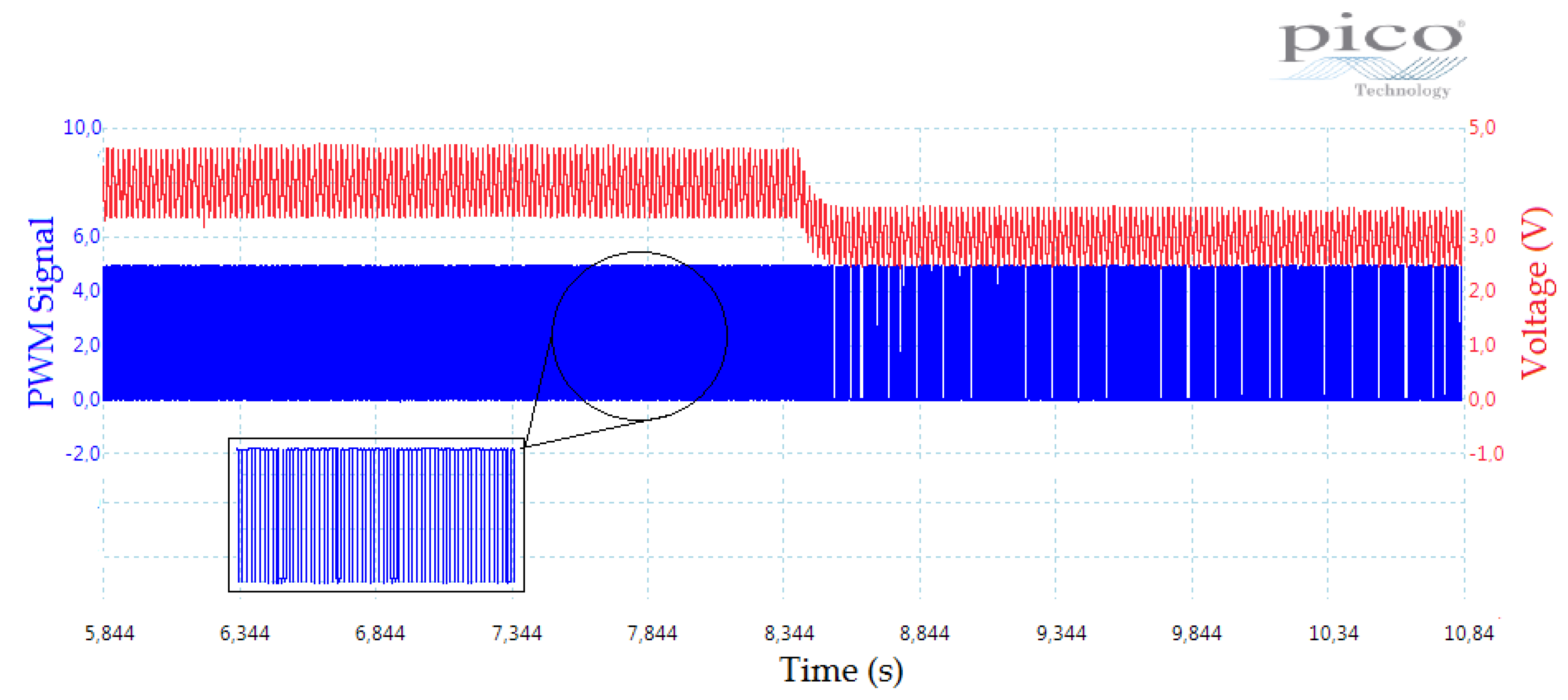
  To successfully complete this stage, it was necessary to modify the Arduino PWM output frequency from 490 Hz to 40 kHz by editing the # PWM Arduino library because of the DC motor dynamics.
• Stage 3: This phase consists of an electronic instrumentation to correctly drive the DC motor (see Figure 7). The PWM control signal generated in Stage 2 ($u_{PWM}$) is a unipolar one since Arduino outputs are limited to positive voltage values. Nevertheless, the DC motor must be able to turn in both senses to increase or decrease the potentiometer resistance linked mechanically to it. For this reason, this stage converts the unipolar signal to a bipolar one without losing the original control signal information.
  Figure 9 shows the final developed platform. Clearly, our experimental platform has notable advantages with respect to other experimental realizations [1,6,20,23,37], such as:
  • It uses low cost electronic components (about 100 Euros).
  • The hardware deployment requires a small area.
  • It is easy to build.
  • It uses an open-source software.

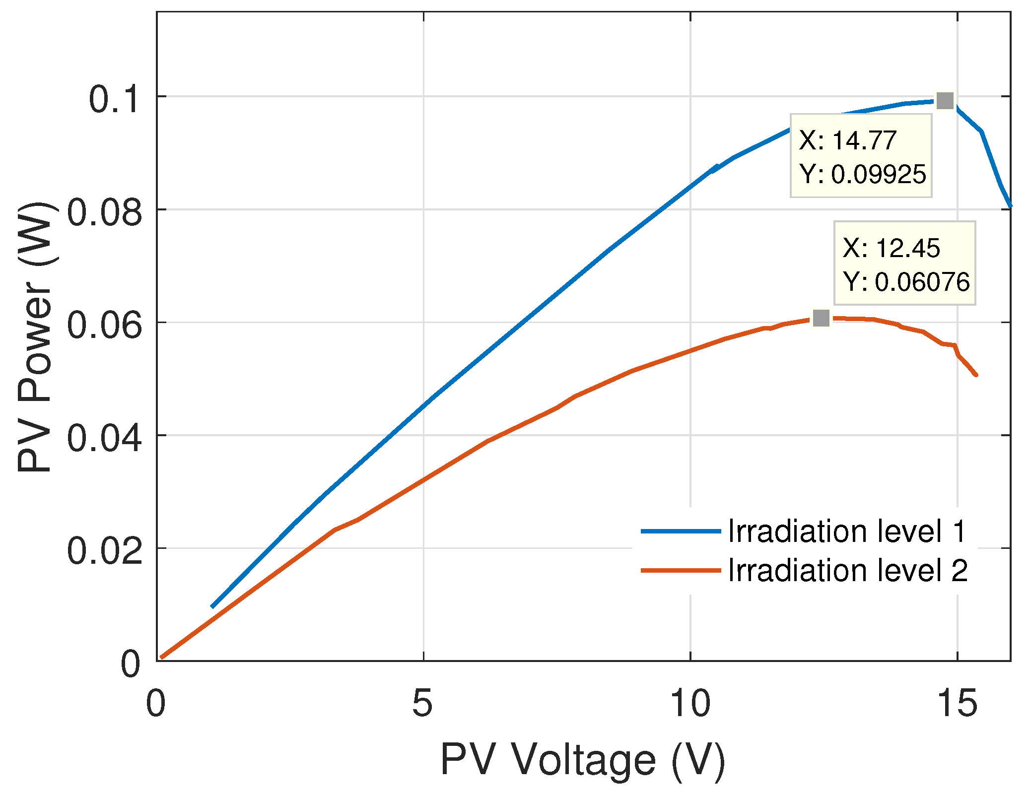
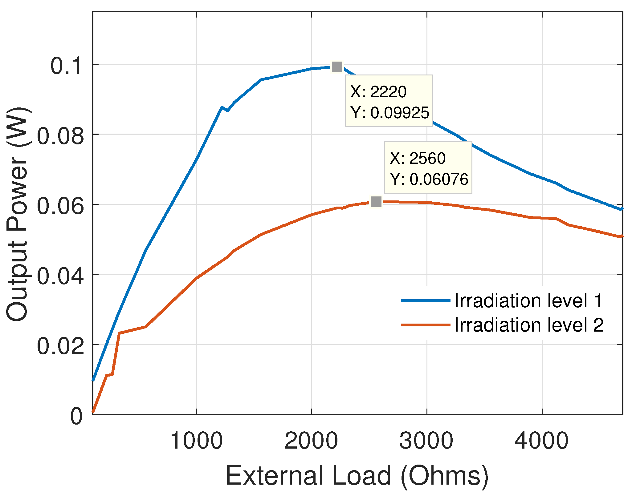
6.2. PV-Panel Characterization

In order to experimentally observe the irradiation effect on the PV panel power, a variation in the load at the PV terminals from 100 $\Omega$ to 4.7 k$\Omega$ was performed for each level of radiation presented in Figure 8. The Tables given in Appendix A summarize the experimental measured values of voltage, current and power for each irradiation level. This experiment allows us to obtain the characteristic curves Voltage-Current, Voltage-Power and Resistance-Power shown in Figure 10, Figure 11 and Figure 12, respectively.

The graphic Voltage-Power in Figure 11 and the curve Resistance-Power in Figure 12 provide evidence that the optimal power point varies for each irradiation condition. In this maximum power point, it is supposed that the external load seen by the PV is similar to the internal resistance in the PV panel [20].

7. Results and Discussion

This section presents the experimental results of the two mentioned MPPT algorithms, the P&O algorithm and the proposed hysteretic MPPT method. Both strategies are implemented in the platform previously described in Section 5. The objective of these experiments is to test the MPPT algorithms and to perform a comparative study between them. These experiments are realized by using the two intensity light levels depicted in Figure 8. Then, the aim is to track, as close as possible, the PV maximum power point corresponding to each light condition (see Figure 12). A PicoScope 2000 Series digital Oscilloscope (PicoScope, Cambridgeshire, UK) is employed to capture the electrical PV waveforms, current, voltage, power and the control signal, at the Board 2 terminals. The experiments are realized in the CoDAlab laboratory at constant temperature (about 22 ${}^{\circ }$C). The parameters for our hysteresis MPPT algorithm were selected by the trial and error strategy. These values were finally set to $\alpha =10$, $a=1$ and $b=1$. For more details, see Appendix C.2.

7.1. Experimental Results by Using the MPPT Perturb and Observer Method

The first result is exposed in Figure 13 where the plots of the PV voltage (blue plot) and the PV current (red plot) signals are shown. The objective of this result is to emphasize that both voltage and current are affected by the light perturbation. A zoomed in version of the above graphic is presented in Figure 14. Here, it is possible to observe an overshoot caused by the control law, the time response and the stabilization time of the PV voltage and PV current, which is approximately one second. Both measured voltage and current signals are the inputs to Arduino; that is, the signals were manipulated to be interpreted by Arduino through the electronic stage with operational amplifiers (see Figure A2). To recover the true PV voltage and PV current values, it is necessary to use the gain factors provided by the operational amplifiers in the circuit previously described in Section 6.1, Stage 1. Then, the gain factors of the PV voltage and PV current values in Figure 13 are 0.468 and 36.96, respectively. Moreover, the corresponding control signal $u_{PWM}$ induced by the P&O algorithm is presented in Figure 15. This figure is representative since it shows the time evolution of the PWM signal produced by the control algorithm in response to the light intensity variation.

Finally, and recalling that the control objective is to achieve, as close as possible, the maximum power point of the PV panel, the PV power plot is exhibited in Figure 16. Note that the power value must be scaled with a factor of 0.057 due to the electronic stage. From this result, the maximum power extracted in the lowest irradiance level is approximately 0.0541 W and the maximum power extracted in the higher irradiance level is approximately 0.0912 W. Both values are close to the maximum power values stated in

Table A1. Measured values for the high irradiation level.

External Load ($\Omega$)	PV Voltage (V)	PV Current (mA)	PV Power (W)
100	1.03	0.0092	0.0095
220	2.14	0.0094	0.0201
270	2.58	0.0094	0.0243
330	3.14	0.0093	0.0294
560	5.20	0.0090	0.0469
1000	8.47	0.0085	0.0728
1220	10.5	0.0083	0.0877
1270	10.41	0.0083	0.0867
1330	10.8	0.0082	0.0891
1560	12.17	0.0078	0.0955
2000	14	0.0070	0.0987
2220	14.77	0.0067	0.0993
2227	14.92	0.0066	0.0989
2330	15.01	0.0065	0.0976
2560	15.45	0.0060	0.0938
3000	15.81	0.0053	0.0843
3270	16.05	0.0049	0.0794
3330	16.03	0.0048	0.0781
3560	16.16	0.0045	0.0739
3900	16.23	0.0042	0.0687
4120	16.34	0.0040	0.0660
4230	16.34	0.0039	0.0641
4460	16.42	0.0037	0.0612
4680	16.48	0.0035	0.0585
4700	16.47	0.0035	0.0590

and

Table A2. Measured values for the low irradiation level.

External Load ($\Omega$)	PV Voltage (V)	PV Current (mA)	PV Power (W)
100	0.0775	0.0071	0.0006
220	1.59	0.0069	0.0111
270	1.63	0.0069	0.0114
330	2.33	0.0069	0.0232
560	3.77	0.0066	0.0250
1000	6.19	0.0062	0.0389
1220	7.28	0.0060	0.0438
1270	7.52	0.0059	0.0450
1330	7.83	0.0059	0.0468
1560	8.90	0.0057	0.0514
2000	10.64	0.0053	0.0570
2220	11.38	0.0051	0.0589
2270	11.5	0.0051	0.0589
2330	11.74	0.0050	0.0596
2560	12.45	0.0048	0.0608
3000	13.42	0.0041	0.0605
3270	13.89	0.0042	0.0596
3330	13.95	0.0042	0.0591
3560	14.36	0.0040	0.0583
3900	14.71	0.0038	0.0562
4120	14.95	0.0037	0.0559
4230	15.02	0.0036	0.0541
4460	15.19	0.0034	0.0524
4680	15.35	0.0033	0.0507
4700	15.30	0.0033	0.0511

.

7.2. Experimental Results by Using the Hysteresis MPPT Method

As in the previous section, the PV voltage and PV current for the two irradiance levels are presented in Figure 17. A close up of voltage and current is presented in Figure 18 where the overshoot seen in the current response in the P&O case was attenuated. In addition, the control signal obtained from Board 2 through the algorithm is shown in Figure 19. This figure is representative since it shows the time evolution of the PWM signal produced by our control algorithm in response to the light intensity variation.

The experimental evaluation is then concluded by showing the PV power graphic depicted in Figure 20. The maximum power extracted with our method in the lowest light level is approximately 0.0556 W and the maximum power extracted in the higher irradiation level is approximately 0.1083 W. Both values are higher than those obtained from the P&O case (see Figure 16). Moreover, they are closer to the maximum power values in Table A1 and Table A2. Observe that the power signal range dynamics in the case with our technique is bigger in comparison to the power signal with the P&O method. However, the peak value is the most important part in some RC-load applications. Note that the graphics in Figure 16 and Figure 20 show negative power raw atypical data introduced by the data acquisition system. This may also be observed, for instance, in [43].

Additionally, to conclude this section, some comments may be drawn from the experimental point of view. First, it is notable that the P&O algorithm is functional as was expected since it is a popular technique in the PV-systems field. However, the results obtained with the proposed MPPT method present an advantage with respect to the P&O results. This is made evident because the proposed method better approaches the optimal maximum PV power as seen in Figure 16 and Figure 20. In addition, it is worth highlighting that the experiments were realized under a repetitive blinking phenomenon, showing that both methods are robust against this light perturbation. This is now an important topic to deal with in the recent literature [25,48,49]. Moreover, our design is exclusively based on a dynamic hysteresis that uses both measurements, the voltage and current of the PV panel. In this way, our algorithm results are efficient enough to extract the maximum power from a PV panel by using low cost electronic realization under the irradiance perturbation. Furthermore, since it uses the voltage and power information from our PV panel, it is able to react to any change in these two variables due to the external light perturbation. Consequently, the new hysteretic model has been crucial in fulfilling our MPPT objective. The proposed algorithm can be interpreted as a hill-climbing method; however, the principal difference between this kind of method and our approach is that the hysteresis provides a memory effect to take into account past states of the variables involved in the system. In addition, our method allows for fixing the response time and other parameters that guarantee a better performance. Summarizing, our MPPT algorithm presents some important advantages with respect to those in the actual state of the art. First, the proposed algorithm employs a dynamic hysteretic equation that takes into account small changes in the PV power and PV voltage measurements. These values jointly work to achieve, as close as possible, the maximum power point. On the other hand, the designed platform is a low cost implementation that allows for testing MPPT algorithms and infer how it works in comparison to other methods. Finally, in our platform, the implementation of our algorithm provides more possibilities of control via software, since the DC-motor controller is directly coded in the programming platform software. This is, in comparison, for instance, to the platform given in [20], our system is an open source for control programming.

8. Conclusions

From the experimental results made evident above, it is concluded that the proposed hysteretic MPPT algorithm provides a better performance than the standard P&O method in PV power regulation under a repetitive blinking phenomenon. This is due to the fact that the hysteresis model produces a smooth behavior with memory effect. Moreover, the proposed algorithm is robust to the light perturbation. To the best knowledge of the authors, this kind of light perturbation is an important topic to study in PV-systems. Additionally, the experimental platform developed in this work presents a novelty because it has a good balance between its low cost electronic design (for instance, the estimated total electronics cost of our design is around 100 Euros) and its adequate performance to test MPPT techniques. Our solution may be instructional for a complete closed-loop design on MPPT by using any programmable digital device and analog electronics. In comparison to the research in the state of the art, our strategy has the novelty of directly employing a dynamic hysteresis equation as the MPPT algorithm. In consequence, the only similitude with other methods, specifically with the different versions of P&O methods, is that it uses information of voltage and current to calculate the supplied PV electrical power. However, in our proposed algorithm, not only is the PV power directly employed in the MPPT algorithm but also the measured PV voltage. This is an important advantage of our method since it is sensitive to any temperature and irradiance change in the PV module that, in collaboration with the smooth hysteresis system, allows for accomplishing the MPPT objective. On the other side, the designed platform has the advantage of being an economical and simple way to test MPPT algorithms. Nevertheless, due to its technical characteristics, it would not be an adequate option to implement in real PV operations’ systems. We believe that our approach may have a positive environmental and economic impact due to its low cost requirement and the possibility to improve the energy conversion efficiency in PV systems. Finally, this paper presents an application-oriented work of a proposed functional MPPT algorithm to extract maximum power from PV panels.

References

- De Brito, M.A.G.; Galotto, L.; Sampaio, L.P.; Melo, G.D.A.; Canesin, C.A. Evaluation of the main MPPT techniques for photovoltaic applications. IEEE Trans. Ind. Electron. 2013, 60, 1156–1167. [Google Scholar] [CrossRef]
- Grätzel, M. Solar energy conversion by dye-sensitized photovoltaic cells. Inorg. Chem. 2005, 44, 6841–6851. [Google Scholar] [CrossRef] [PubMed]
- Carreño-Ortega, A.; Galdeano-Gómez, E.; Pérez-Mesa, J.C.; Galera-Quiles, M.D.C. Policy and environmental implications of photovoltaic systems in farming in southeast Spain: Can greenhouses reduce the greenhouse effect? Energies 2017, 10, 761. [Google Scholar] [CrossRef]
- Hassan, A.S.; Cipcigan, L.; Jenkins, N. Optimal battery storage operation for PV systems with tariff incentives. Appl. Energy 2017, 203, 422–441. [Google Scholar] [CrossRef]
- Vieira, F.M.; Moura, P.S.; de Almeida, A.T. Energy storage system for self-consumption of photovoltaic energy in residential zero energy buildings. Renew. Energy 2017, 103, 308–320. [Google Scholar] [CrossRef]
- Boukenoui, R.; Ghanes, M.; Barbot, J.P.; Bradai, R.; Mellit, A.; Salhi, H. Experimental assessment of Maximum Power Point Tracking methods for photovoltaic systems. Energy 2017, 132, 324–340. [Google Scholar] [CrossRef]
- Karami, N.; Moubayed, N.; Outbib, R. General review and classification of different MPPT Techniques. Renew. Sustain. Energy Rev. 2017, 68, 1–18. [Google Scholar] [CrossRef]
- Schwertner, C.D.; Bellinaso, L.V.; Hey, H.L.; Michels, L. Supervisory control for stand-alone photovoltaic systems. In Proceedings of the 2013 Brazilian Power Electronics Conference (COBEP), Gramado, Brazil, 27–31 October 2013; pp. 582–588. [Google Scholar]
- Yang, Y.; Blaabjerg, F.; Wang, H.; Simoes, M.G. Power control flexibilities for grid-connected multi-functional photovoltaic inverters. IET Renew. Power Gener. 2016, 10, 504–513. [Google Scholar] [CrossRef] [Green Version]
- Cucchiella, F.; D’Adamo, I.; Gastaldi, M. Economic analysis of a photovoltaic system: A Resource for residential households. Energies 2017, 10, 814. [Google Scholar] [CrossRef]
- Liu, J.; Long, Y.; Song, X. A study on the conduction mechanism and evaluation of the comprehensive efficiency of photovoltaic power generation in China. Energies 2017, 10, 723. [Google Scholar]
- Hernández, J.C.; Bueno, P.G.; Sanchez-Sutil, F. Enhanced utility-scale photovoltaic units with frequency support functions and dynamic grid support for transmission systems. IET Renew. Power Gener. 2017, 11, 361–372. [Google Scholar] [CrossRef]
- Koutroulis, E.; Blaabjerg, F. A new technique for tracking the global maximum power point of PV arrays operating under partial-shading conditions. IEEE J. Photovolt. 2012, 2, 184–190. [Google Scholar] [CrossRef]
- Hemandez, J.; Garcia, O.; Jurado, F. Photovoltaic devices under partial shading conditions. Int. Rev. Model. Simul. 2012, 5, 414–425. [Google Scholar]
- Rodrigues, E.; Osório, G.; Godina, R.; Bizuayehu, A.; Lujano-Rojas, J.; Catalão, J. Grid code reinforcements for deeper renewable generation in insular energy systems. Renew. Sustain. Energy Rev. 2016, 53, 163–177. [Google Scholar] [CrossRef]
- Cabrera-Tobar, A.; Bullich-Massagué, E.; Aragüés-Peñalba, M.; Gomis-Bellmunt, O. Review of advanced grid requirements for the integration of large scale photovoltaic power plants in the transmission system. Renew. Sustain. Energy Rev. 2016, 62, 971–987. [Google Scholar] [CrossRef]
- Orchi, T.F.; Mahmud, M.A.; Oo, A.M.T. Generalized dynamical modeling of multiple photovoltaic units in a grid-connected system for analyzing dynamic interactions. Energies 2018, 11, 296. [Google Scholar] [CrossRef]
- Ni, Q.; Zhuang, S.; Sheng, H.; Wang, S.; Xiao, J. An optimized prediction intervals approach for short term PV power forecasting. Energies 2017, 10, 1669. [Google Scholar] [CrossRef]
- Kim, D.J.; Kim, B.; Ko, H.S.; Jang, M.S.; Ryu, K.S. A novel supervisory control algorithm to improve the performance of a real-time PV power-hardware-in-loop simulator with Non-RTDS. Energies 2017, 10, 1651. [Google Scholar] [CrossRef]
- Kebir, A.; Woodward, L.; Akhrif, O. Extremum-seeking control with adaptive excitation: Application to a photovoltaic system. IEEE Trans. Ind. Electron. 2018, 65, 2507–2517. [Google Scholar] [CrossRef]
- Marinkov, S.; de Jager, B.; Steinbuch, M. Extremum seeking control with data-based disturbance feedforward. In Proceedings of the 2014 American Control Conference (ACC), Portland, OR, USA, 4–6 June 2014; pp. 3627–3632. [Google Scholar]
- Ouoba, D.; Fakkar, A.; El Kouari, Y.; Dkhichi, F.; Oukarfi, B. An improved maximum power point tracking method for a photovoltaic system. Opt. Mater. 2016, 56, 100–106. [Google Scholar] [CrossRef]
- Farhat, M.; Barambones, O.; Sbita, L. A new maximum power point method based on a sliding mode approach for solar energy harvesting. Appl. Energy 2017, 185, 1185–1198. [Google Scholar] [CrossRef]
- Femia, N.; Petrone, G.; Spagnuolo, G.; Vitelli, M. Power Electronics and Control Techniques for Maximum Energy Harvesting in Photovoltaic Systems; CRC Press: Boca Raton, FL, USA, 2017. [Google Scholar]
- Belkaid, A.; Colak, I.; Isik, O. Photovoltaic maximum power point tracking under fast varying of solar radiation. Appl. Energy 2016, 179, 523–530. [Google Scholar] [CrossRef]
- Safari, A.; Mekhilef, S. Simulation and hardware implementation of incremental conductance MPPT with direct control method using cuk converter. IEEE Trans. Ind. Electron. 2011, 58, 1154–1161. [Google Scholar] [CrossRef]
- Elgendy, M.A.; Zahawi, B.; Atkinson, D.J. Assessment of perturb and observe MPPT algorithm implementation techniques for PV pumping applications. IEEE Trans. Sustain. Energy 2012, 3, 21–33. [Google Scholar] [CrossRef]
- Robles Algarín, C.; Taborda Giraldo, J.; Rodríguez Álvarez, O. Fuzzy logic based MPPT controller for a PV system. Energies 2017, 10, 2036. [Google Scholar] [CrossRef]
- Enany, M.A.; Farahat, M.A.; Nasr, A. Modeling and evaluation of main maximum power point tracking algorithms for photovoltaics systems. Renew. Sustain. Energy Rev. 2016, 58, 1578–1586. [Google Scholar] [CrossRef]
- Dochain, D.; Perrier, M.; Guay, M. Extremum seeking control and its application to process and reaction systems: A survey. Math. Comput. Simul. 2011, 82, 369–380. [Google Scholar] [CrossRef]
- Tafticht, T.; Agbossou, K.; Doumbia, M.; Cheriti, A. An improved maximum power point tracking method for photovoltaic systems. Renew. Energy 2008, 33, 1508–1516. [Google Scholar] [CrossRef]
- Dasgupta, N.; Pandey, A.; Mukerjee, A.K. Voltage-sensing-based photovoltaic MPPT with improved tracking and drift avoidance capabilities. Sol. Energy Mater. Sol. Cells 2008, 92, 1552–1558. [Google Scholar] [CrossRef]
- Scarpa, V.V.; Buso, S.; Spiazzi, G. Low-complexity MPPT technique exploiting the PV module MPP locus characterization. IEEE Trans. Ind. Electron. 2009, 56, 1531–1538. [Google Scholar] [CrossRef]
- Hammami, M.; Grandi, G. A single-phase multilevel PV generation system with an improved ripple correlation control MPPT algorithm. Energies 2017, 10, 2037. [Google Scholar] [CrossRef]
- Liu, F.; Kang, Y.; Zhang, Y.; Duan, S. Comparison of P&O and hill climbing MPPT methods for grid-connected PV converter. In Proceedings of the 2008 3rd IEEE Conference on Industrial Electronics and Applications (ICIEA 2008), Singapore, 3–5 June 2008; pp. 804–807. [Google Scholar]
- Liu, F.; Duan, S.; Liu, F.; Liu, B.; Kang, Y. A variable step size INC MPPT method for PV systems. IEEE Trans. Ind. Electron. 2008, 55, 2622–2628. [Google Scholar]
- Loukriz, A.; Haddadi, M.; Messalti, S. Simulation and experimental design of a new advanced variable step size Incremental Conductance MPPT algorithm for PV systems. ISA Trans. 2016, 62, 30–38. [Google Scholar] [CrossRef] [PubMed]
- Leyva, R.; Alonso, C.; Queinnec, I.; Cid-Pastor, A.; Lagrange, D.; Martínez-Salamero, L. MPPT of photovoltaic systems using extremum-seeking control. IEEE Trans. Aerosp. Electron. Syst. 2006, 42, 249–258. [Google Scholar] [CrossRef]
- Mao, M.; Duan, Q.; Duan, P.; Hu, B. Comprehensive improvement of artificial fish swarm algorithm for global MPPT in PV system under partial shading conditions. Trans. Inst. Meas. Control 2018, 40, 2178–2199. [Google Scholar] [CrossRef]
- Mellit, A.; Kalogirou, S.A. MPPT-based artificial intelligence techniques for photovoltaic systems and its implementation into field programmable gate array chips: Review of current status and future perspectives. Energy 2014, 70, 1–21. [Google Scholar] [CrossRef]
- Chen, Y.T.; Jhang, Y.C.; Liang, R.H. A fuzzy-logic based auto-scaling variable step-size MPPT method for PV systems. Sol. Energy 2016, 126, 53–63. [Google Scholar] [CrossRef]
- Faranda, R.; Leva, S. Energy comparison of MPPT techniques for PV systems. WSEAS Trans. Power Syst. 2008, 3, 446–455. [Google Scholar]
- Aranda, E.D.; Galan, J.A.G.; De Cardona, M.S.; Marquez, J.M.A. Measuring the IV curve of PV generators. IEEE Ind. Electron. Mag. 2009, 3, 4–14. [Google Scholar] [CrossRef]
- Verneau, G.; Aubard, L.; Crebier, J.C.; Schaeffer, C.; Schanen, J.L. Empirical power MOSFET modeling: Practical characterization and simulation implantation. In Proceedings of the 37th IAS Annual Meeting, Conference Record of the 2012 IEEE Industry Applications Conference, Pittsburgh, PA, USA, 13–18 October 2002; pp. 2425–2432. [Google Scholar]
- Acho, L.; Vidal, Y. Hysteresis modeling of a class of RC-OTA hysteretic-chaotic generators. In Proceedings of the 5th International Conference on Physics and Control, León, Spain, 5–8 September 2011. [Google Scholar]
- Tutivén, C.; Vidal, Y.; Acho, L.; Rodellar, J. Hysteresis-based design of dynamic reference trajectories to avoid saturation in controlled wind turbines. Asian J. Control 2017, 19, 438–449. [Google Scholar] [CrossRef]
- De León, N.I.P.; Acho, L.; Rodellar, J. Adaptive predictive control of a base-isolated hysteretic system. In Proceedings of the 2017 21st International Conference on System Theory, Control and Computing (ICSTCC), Sinaia, Romania, 19–21 October 2017; pp. 390–395. [Google Scholar]
- Manickam, C.; Raman, G.P.; Raman, G.R.; Ganesan, S.I.; Chilakapati, N. Fireworks enriched P&O algorithm for GMPPT and detection of partial shading in PV systems. IEEE Trans. Power Electron. 2017, 32, 4432–4443. [Google Scholar]
- Das, P.; Mohapatra, A.; Nayak, B. Modeling and characteristic study of solar photovoltaic system under partial shading condition. Mater. Today Proc. 2017, 4, 12586–12591. [Google Scholar] [CrossRef]
© 2018 by the authors. Licensee MDPI, Basel, Switzerland. This article is an open access article distributed under the terms and conditions of the Creative Commons Attribution (CC BY) license (http://creativecommons.org/licenses/by/4.0/).
Share and Cite
Ponce de León Puig, N.I.; Acho, L.; Rodellar, J. Design and Experimental Implementation of a Hysteresis Algorithm to Optimize the Maximum Power Point Extracted from a Photovoltaic System. Energies 2018, 11, 1866. https://doi.org/10.3390/en11071866
Ponce de León Puig NI, Acho L, Rodellar J. Design and Experimental Implementation of a Hysteresis Algorithm to Optimize the Maximum Power Point Extracted from a Photovoltaic System. Energies. 2018; 11(7):1866. https://doi.org/10.3390/en11071866
Chicago/Turabian StylePonce de León Puig, Nubia Ilia, Leonardo Acho, and José Rodellar. 2018. "Design and Experimental Implementation of a Hysteresis Algorithm to Optimize the Maximum Power Point Extracted from a Photovoltaic System" Energies 11, no. 7: 1866. https://doi.org/10.3390/en11071866