Optimization Scheduling Method for Power Systems Considering Optimal Wind Power Intervals


School of Electrical Engineering, Wuhan University, Wuhan 430072, China
*
Author to whom correspondence should be addressed.
Energies 2018, 11(7), 1710; https://doi.org/10.3390/en11071710
Submission received: 7 May 2018
/
Revised: 13 June 2018
/
Accepted: 17 June 2018
/
Published: 1 July 2018
(This article belongs to the Section F: Electrical Engineering)
Abstract
:Wind power intervals with different confidence levels have an impact on both the economic cost and risk of dispatch plans for power systems with wind power integration. The higher the confidence level, the greater the bandwidth of corresponding intervals. Thus, more reserves are needed, resulting in higher economic cost but less risk. In order to balance the economic cost and risk, a unit commitment model based on the optimal wind power confidence level is proposed. There are definite integral terms in the objective function of the model, and both the integrand function and integral upper/lower bound contain decision variables, which makes it difficult to solve this problem. The objective function is linearized and solved by discretizing the wind power probability density function and using auxiliary variables. On the basis, a rolling dispatching model considering the dynamic regulation costs among multiple rolling plans is established. In addition to balancing economic cost and risk, it can help to avoid repeated regulations among different rolling plans. Simulations are carried on a 10-units system and a 118-bus system to verify the effectiveness of the proposed models.
1. Introduction
Due to its inherent intermittency and volatility, the integration of large-scale wind power brings great uncertainty to power systems, and it challenges the formulation of scheduling plans for power systems. Traditional scheduling models use wind power point prediction information to arrange the units’ output and cannot fully take the uncertainty of wind power into account. More reserves are needed to keep power balance in power system, which certainly impose higher operation costs. In order to deal with the wind power uncertainty, a lot of researches have been conducted. Stochastic optimization (SO) [1], chance-constrained optimization (CCO) [2], robust optimization (RO) [3] and interval optimization (IO) [4] are the most commonly used methods.
The main idea of SO is to generate a large set of scenarios by sampling the probability distribution of wind power, and then eliminate the part of these scenarios with low probability. Thus, the remaining typical scenarios along with their probabilities are used to model the wind power uncertainty. The disadvantage of SO is that it depends on the accuracy of probability distribution of wind power uncertainty and the selected scenarios. In the CCO method, the solution can violate the system security constraints to some extent, but the probability that the solution should satisfy the constraints is not less than a certain predefined confidence level. The optimality of a CCO solution also relies on the probability distribution of uncertain variables which is problematic in real-world applications [5]. RO does not require any assumptions about the probability distribution of uncertain variables and allows fluctuations of wind power within a given range. However, its solution tends to be conservative for that its objective is to minimize the cost of the worst-case scenario. IO generates the upper and lower boundaries of generation dispatch. It requires less computation, but the results are still conservative and not precise enough [6].
The above methods have their own advantages and disadvantages, but these methods are all based on given wind power confidence levels. For example, the SO method in [7] generates the scenarios within upper and lower boundaries of the 95% confidence intervals. RO and IO usually only focus on the circumstances that may occur within the interval boundary, regardless of the confidence level, or only consider the interval with a given confidence level [5,8,9]. In summary, these methods usually set the interval boundary with a fixed confidence level such as 90% [10], or set the interval boundary to ±20% [11] of predictive values, or 20% [12] of the installed capacity and so on.
Generally speaking, the wind power forecasting interval with a high confidence level tends to have a greater bandwidth. That is, the possible fluctuation range of wind power is larger, and thus more reserves are needed, but the risks of wind curtailment and load shedding are smaller. In a word, the higher confidence level leads to greater economic cost but smaller risk. How to balance the economic cost and risk of system is a problem that worth studying. A RO dispatch model with adjustable uncertainty sets is established in [13] to reduce the conservativeness, and the dispatch costs along with the wind power confidence levels varying from 60% to 95% are calculated. It can be seen that the economic cost and risk of the solutions vary with the confidence levels. A wind power adjustable interval based model for scheduling the energy and reserve is proposed in [6], and it shows better performance than traditional models based on prediction intervals. However, it is pointed out in [14] that this study regards wind power unschedulable and it uses a Gaussian distribution to simulate wind power uncertainty, which may lead to a more expensive schedule.
Since there exists a complementary relationship between the economic cost and risk of the power system dispatch plan as the wind power confidence level changes, there should be an optimal confidence level that balance the two. Therefore, from the perspective of wind power confidence level, a unit commitment (UC) model based on optimal wind power intervals is proposed in this paper. The results can provide reference for the selection of wind power optimal confidence intervals in the UC problem and the selection of confidence level in wind power interval forecasting.
On the basis of day-ahead UC model, an intra-day rolling dispatch model is established to revise the deviations of the pre-day plan for that the forecast accuracy of wind power increases as the time scale decreases. A look-ahead economic dispatch approach is proposed in [15] with the objective of minimizing the total production cost. For each sub-period, based on the latest forecast information for a prespecified time horizon, the look-ahead dispatch model formulates a dispatch plan in a rolling manner [16], and only the results of the first one or several periods are actually executed. However, the conventional look-ahead dispatch models always aim at the optimal operation cost and lack the overall optimality within the entire scheduling periods. Therefore, this paper introduces the dynamic adjustment costs, which takes into account the man power and material resources required for the regulation of the dispatch plans, and it can help to reduce the regulation quantity among different rolling dispatch plans.
In summary, the major contributions of this paper are as follows:
- (1)
- A UC model considering the optimal wind power confidence intervals is established to balance the economic costs and risk of the dispatch plan for the power system with wind power integration.
- (2)
- The UC model is a mixed integer nonlinear programming (MINLP) problem with integral terms in its objective, and both the integrand function and integral upper/lower bound contain decision variables. The objective function is linearized and solved by discretizing the wind power probability density function and using auxiliary variables.
- (3)
- Based on the UC model, in addition to optimal wind power confidence intervals, the dynamic adjustment cost is introduced into intra-day rolling dispatch model to reduce the amount of adjustments among different rolling dispatch plans.
2. Overall Framework and Representation of Wind Power Uncertainty
2.1. Overall Framework
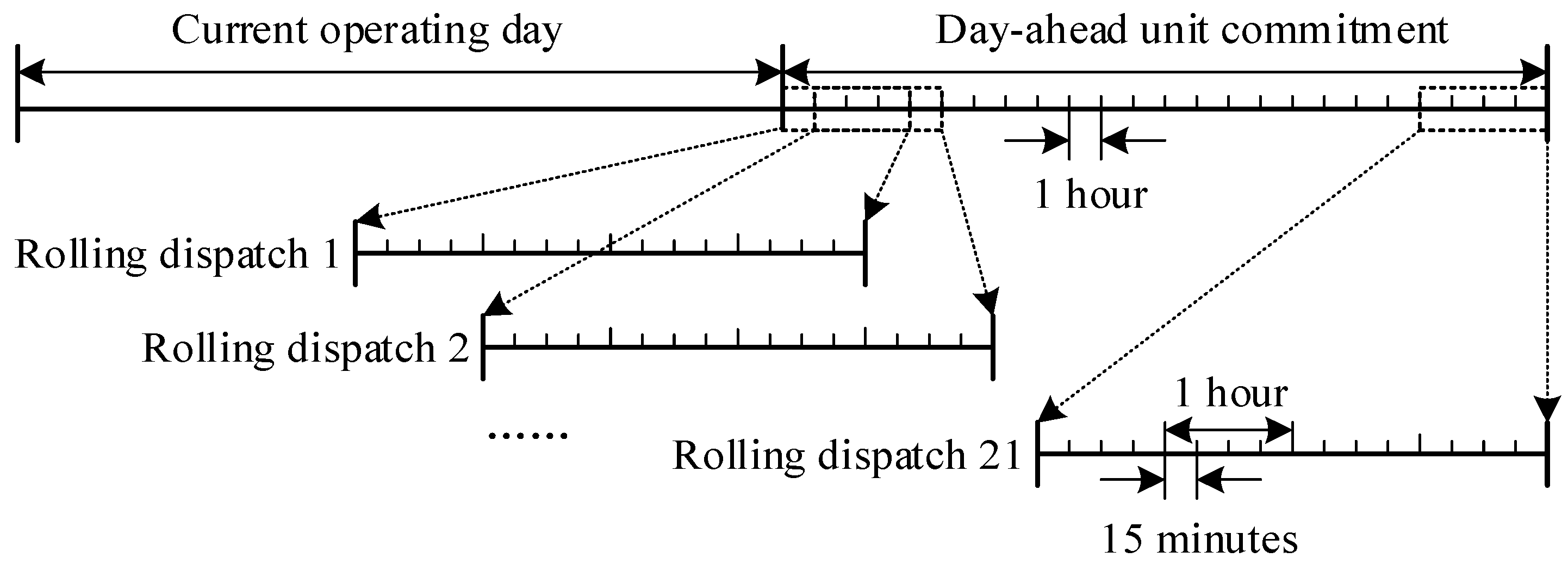
A dispatch strategy with two time-scale modules is developed in this paper, including the day-ahead UC and the intra-day rolling dispatch. The framework of the strategy is shown in Figure 1 and depicted below.
- (1)
- Day-ahead UC. It is a mixed integer nonlinear programming problem with the goal of minimizing the economic cost and risk cost. The UC for the next operating day is performed in current operation day, and it provides the UC plan of 24 h for the next day.
- (2)
- Intra-day rolling dispatch. Based on the latest load and wind power forecasting information, it is activated every 1 h to modify the power generation output of the next 4 h in a rolling manner. In each rolling plan, only the dispatch plan of the first hour is actually executed.
2.2. Representation of Wind Power Uncertainty
At present, most wind power forecasting systems provide predictive results in the form of point forecasting. To estimate the confidence intervals of wind power, it is necessary to obtain the conditional distribution of the wind power output with respect to the point forecasting value, that is, the conditional probability distribution of the possible output under the condition of “known point forecasting value”.
In order to obtain the probability distribution, the idea of “forecast bin” in [17] is used in this paper. At first, the historical wind power data along with its predictive value are formed as a row vector in the form of [predictive value, measured value]. Assuming there are N sets of data, an N × 2 matrix is eventually formed. The matrix is normalized, and all the row vectors are ranked in ascending order in accordance with the predictive values. Then the wind power forecast domain (i.e., [0, 1] p.u.) is divided into M evenly distributed bins which are called forecast bins (FB). The value of M is determined by the size of N, and it is set as 50 in this paper. The width of each FB is 0.02 p.u., that is, the range of the forecast values in the first FB is [0, 0.02] p.u., and that in the FB m (m = 1, 2, …, M) is [(m − 1)/50, m/50] p.u.. Thus, the values of the predictive values in each FB are similar, while the actual values are generally quite different. Then the probability distribution of the possible wind power output in each FB can be obtained by counting the actual measured values. When the predictive value is known, it is compared with the range of each FB. If it falls within a certain FB, it’s in accordance with the probability distribution of the FB.
In the distribution statistics of the data, there are two kinds of models: parameter distribution models and non-parameter distribution models. The parameter distribution models include normal distribution, beta distribution, etc. However, in reality, it is difficult to find a reasonable parameter distribution for that different prediction methods are applied on different wind farms, and the distribution of prediction errors are different as well. Therefore, it is not reasonable to simply assume that the measured values in the FB obey a certain probability distribution. A non-parametric empirical distribution model is used to simulate the distribution of the measured values. The main advantage of this method is that it is not necessary to assume any specific distribution of random variables. Sufficient historical data are needed to approximate the probability distribution.
If the measured values in a FB are ranked in ascending order as , then the empirical probability distribution function (PDF) of the wind power in the FB is as follows[17]:
When the number of samples n in Equation (1) is large enough, the empirical distribution function is close to the theoretical distribution. Based on the empirical probability distribution, the intervals with different confidence levels can be calculated. For example, the quantiles corresponding to 0.025 and 0.975 in the PDF are the lower and upper interval boundaries with 95% confidence level. Thus, the intervals with confidence levels from 1% to 99% can be obtained.
3. The Proposed Model
3.1. UC Model Based on Optimal Conficence Level
3.1.1. Objective
The objective function of the UC model which does not consider the wind power confidence interval is to minimize fuel cost, on-off cost and reserve cost, etc. In addition to the plan for wind power point predictive value, the UC scheme based on optimal wind power confidence level needs to consider any circumstances that may occur in the interval, as well as the risk that the actual value falls outside the interval. Taking into account the impact of wind power intervals with different confidence levels on the UC scheme, an objective function is proposed and shown in Equation (3):
where i is the number of thermal power units. j is the number of wind farms. t is the period number. NT is the total number of the periods. NG is the total number of thermal power units. NW is the number of wind farms. is the fuel cost of thermal power units i in period t and its expression is shown in Equation (4). is the reserve cost of unit i in period t, and the expression is shown in Equation (5). is the start-up cost of unit i in period t, and the expression is shown in Equation (6). is the cost incurred by wind farm j in period t, and the expression is shown in Equation (9):
where ai, bi and ci are the cost coefficients of the thermal power unit i. Pi,t is the dispatching power of the thermal power unit i in period t. and are the upward and downward reserve cost coefficient for unit i. and are the upward and downward reserves provided by unit i in period t, is the starting cost constant for unit i, Ii,t is a binary variable which indicates the unit’s on/off status.
in Equation (4) is a nonlinear term, and it is linearized by piecewise linearization. The expression is as follows:
where Nm is the number of segments. is the fuel cost corresponding to the minimum output of the unit i. Ki,t,m is the slope of the unit i at the segment m in period t. Pi,t,m is the output of unit i at the segment m in period t. Binary variables ui,t and vi,t are introduced to linearize in Equation (6). ui,t is the start-up status variable, for which 1 means that the unit is in the boost process. For the shut-down status variable vi,t, 1 represents that the unit is in the shut-down process. Thus, Equation (6) can be transformed into the linear expression shown in Equation (8):
Figure 2 shows the probability density distribution curve of wind power, in which , and represent the scheduled wind power, upper and lower bound of confidence interval at time t, respectively.
If the actual output of wind power is located within the boundary of the interval , the wind power prediction error can be compensated by the upward and downward reserves. If the actual output exceeds the boundary, the wind power uncertainty cannot be covered by system reserves, and wind curtailment or load shedding will be used to ensure the safe operation of the system. The wider the confidence interval is, the more reserves are needed for the system, but the smaller the risks of wind curtailment and load shedding. Therefore, the cost of actual reserves and risk cost caused by wind power uncertainty are introduced into the objective function in this paper.
It can be seen from the figure that the three variables divide the probability density curve into four parts, the first part is [0, ], the area of the shaded part represents the expected load shedding probability due to wind power under estimation. The second part is [, ], and the wind power errors in this part which is caused by under estimation can be covered by upward reserves of system. The third part is [, ], and the uncertainties in this part caused by the wind power overestimation can be covered by downward reserves. The fourth part is [, 1], the area of the shaded part represents the expected wind curtailment probability caused by wind power overestimation. Therefore, the cost caused by wind power uncertainty can be expressed as follows:
where f(x) is the probability density distribution function. , , and are the expected load shedding caused by wind power overestimation (OVLS), the expected overestimation wind power that can be covered by upward reserve (OVUR), the expected underestimation wind power that can be covered by downward reserve (UNDR), the expected wind curtailment caused by wind power underestimation (UNWC), respectively. , , and are their corresponding cost coefficients.
It is worth noting that the OVUR include both [, ] part and [0, ] part. Since the uncertainty in [0, ] is also covered by upward reserve, and the upward reserve is used up so that partial load has to be cut to maintain the power balance of power system. Similarly, the UNDR also include the [, 1] part.
3.1.2. Constraints
The constraints are as follows:
- (1)
- Supply-demand balance constraints:where Pi,t is the active output of unit i in period t. wj,t is the schedule value of wind farm j in period t. is the load forecast value in period t.
- (2)
- Thermal power plants output constraints:where and are the upper and lower limits of the output of unit i.
- (3)
- Unit segment output constraints:where is the maximum output of unit i on segment m.
- (4)
- Unit ramping up and down constraints:where URi, DRi are the maximum up and down ramp rate of unit i.
In addition to Equations (15) and (16), it is necessary to consider any circumstances where the wind power output changes within the confidence intervals. For example, when wind power jumps from the confidence interval boundary of the current time period to the boundary of next time period, it is also necessary to ensure that the conventional units have sufficient adjustment capability to ensure the safe operating of the system. Therefore, Equations (17)–(20) are also considered in this model, representing the two extreme cases shown in Figure 3:
- (5)
- Unit minimum ON and OFF time limits:where and are the minimum start-up time and shut-down time for unit i, respectively.
- (6)
- Unit upward and downward reserves constraints:
The wind power uncertainty within the lower and upper boundaries of the confidence intervals is considered to be covered by system reserves, so that Equations (25) and (26) are also included:
3.2. Rolling Dispatch Model
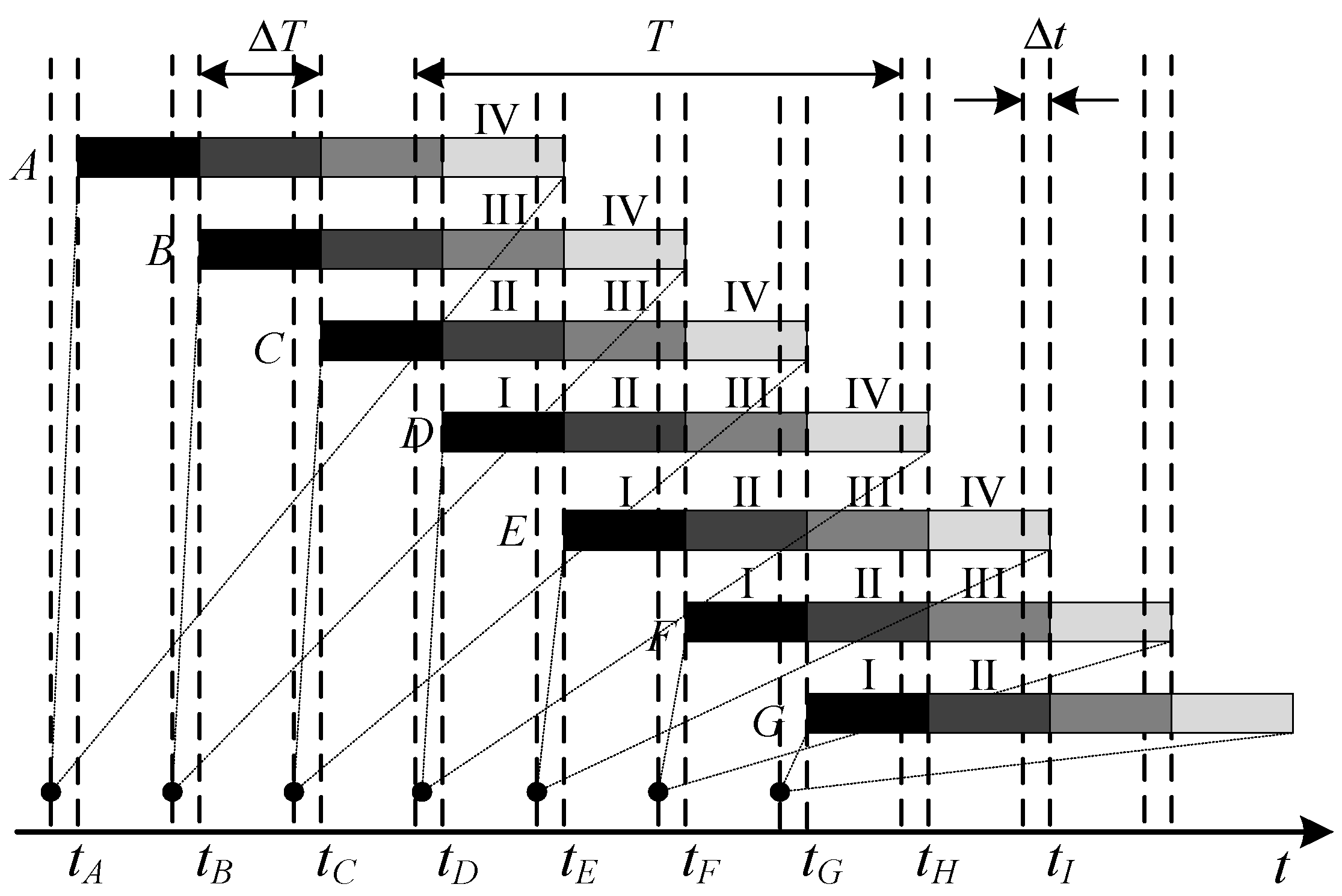
As the wind power prediction accuracy increases with decreasing time scale, the intra-day rolling schedule based on the latest wind power forecasting value can help to reduce the deviation of the day-ahead plan. As shown in Figure 4, = 15 min, T = 4 h, = 1 h. The rolling plan is formulated every 15 min before the scheduled time, and a plan for 4 h is formulated. The plan is executed every 1 h, and the plan for the first 1 h out of 4 h will be actually executed every time.
Generally, the rolling dispatch model only optimizes the cost of each rolling plan, and lacks the consideration of coordination among multiple rolling plans, which affects the global optimality in the overall scheduling periods. Therefore, the coordination among various rolling plans is considered in this paper. Taking tD–tE period as an example, when formulating the first rolling plan at time , the wind power prediction accuracy for this period is not high enough so that the confidence level is not strictly required. When formulating the fourth rolling plan at time , the confidence level needs to be strictly met. In addition to the fuel cost and risk cost, the regulation cost is also introduced in the objective function of the model. The purpose is to reduce the overall amount of regulations and avoid repeated regulations among the rolling plans.
3.2.1. Objective
Taking tD–tH periods as an example, the objective function of this rolling plan includes the regulation costs of CII to DI, CIII to DII, CIV to DIII, and the day-ahead plan of tG–tH period to DIV, in addition to the fuel costs and risk costs of DI, DII, DIII, and DIV periods. Similarly, the objective function of the next rolling plan includes the fuel costs and risk costs of the EI, EII, EIII, and EIV periods, the regulation costs of DII-EI, DIII-EII, DIV-EIII, and the day-ahead plan of tH–tI period to EIV. It is worth noting that this is only the cost of the objective function, rather than the actual scheduling cost within the overall scheduling periods. At the time tD, only the wind power and load forecasting values in DI, DII, DIII, and DIV periods are known, the fuel cost and risk costs of these four periods are included in the objective function. However, the actual total cost within tD–tH includes the fuel costs and risk costs of DI, EI, FI, and GI periods, and the corresponding regulation costs for each period, such as the tD–tE period with four regulation costs (day-ahead plan of tD–tE period to AIV, AIV to BIII, BIII to CII, CII to DI). Therefore, there are 16 regulations in the tD–tH periods.
The intra-day rolling plan does not change the day-ahead unit commitment, and it is essentially a dynamic economic dispatch problem. The objective function includes the fuel cost, reserve cost, risk cost, and regulation cost, and it is expressed as follows:
where is the regulation cost of the unit i in period t, and its expression is shown in Equation (28). The expression of in Equation (27) is different from Equation (9) for that a penalty factor μ is introduced to coordinate the risks among different rolling plans, and it is shown in Equation (29):
where is the cost coefficient of output regulation, l = 1, 2, 3, 4 which represent the I, II, III, IV periods in a rolling plan. is the output regulation amount of the unit I at time t in the k-th rolling plan. is the output of the unit i at time t in the k-th rolling plan. is the output of the last rolling plan at time . is the day-ahead output corresponding to the time t in the k-th rolling plan. This formula reflects that the regulation amount for each rolling plan is the output of this plan minus the output of the previous plan, and if there is no plan for the previous time, the minuend is the output of day-ahead plan.
3.2.2. Constraints
Considering that the scheduled power of the rolling plan is related to the daily plan and the previous rolling plan, the regulation quantity of the rolling plan should not be too large, and the deviation of the correction value needs to be controlled within a certain range:
where , are the maximum values of the upward regulation and the downward regulation in the k-th rolling plan of unit i at the time t. and are the amounts of maximum upward and downward regulation allowed for the unit i.
The penalty factor needs to satisfy the following constraint:
Other constraints can refer to the content of the UC model which is shown in Equations (9)–(24). The decision variables of the model are the output , the upward/downward reserve , and the wind power dispatch value .
3.3. Model Transformation and Solution
The decision variables of the proposed UC model are the binary variables Ii,t, ui,t and vi,t which indicate the unit’s on/off, start-up and shut-down status, the scheduled power Pi,t, the upward/downward reserve /, the scheduled wind power , and the upper/lower boundary of confidence interval /. The UC model is a mixed integer nonlinear programming problem (MINLP). There are definite integral terms in the objective function of the model, and both the integrand function and integral upper/lower bound contain decision variables, which makes it difficult to solve this problem. Therefore, it is necessary to linearize the integral terms of the objective function.
Take the first two terms in Equation (9) as an example, set . Divide the probability density function into S segments, then the following equivalent expression can be obtained:
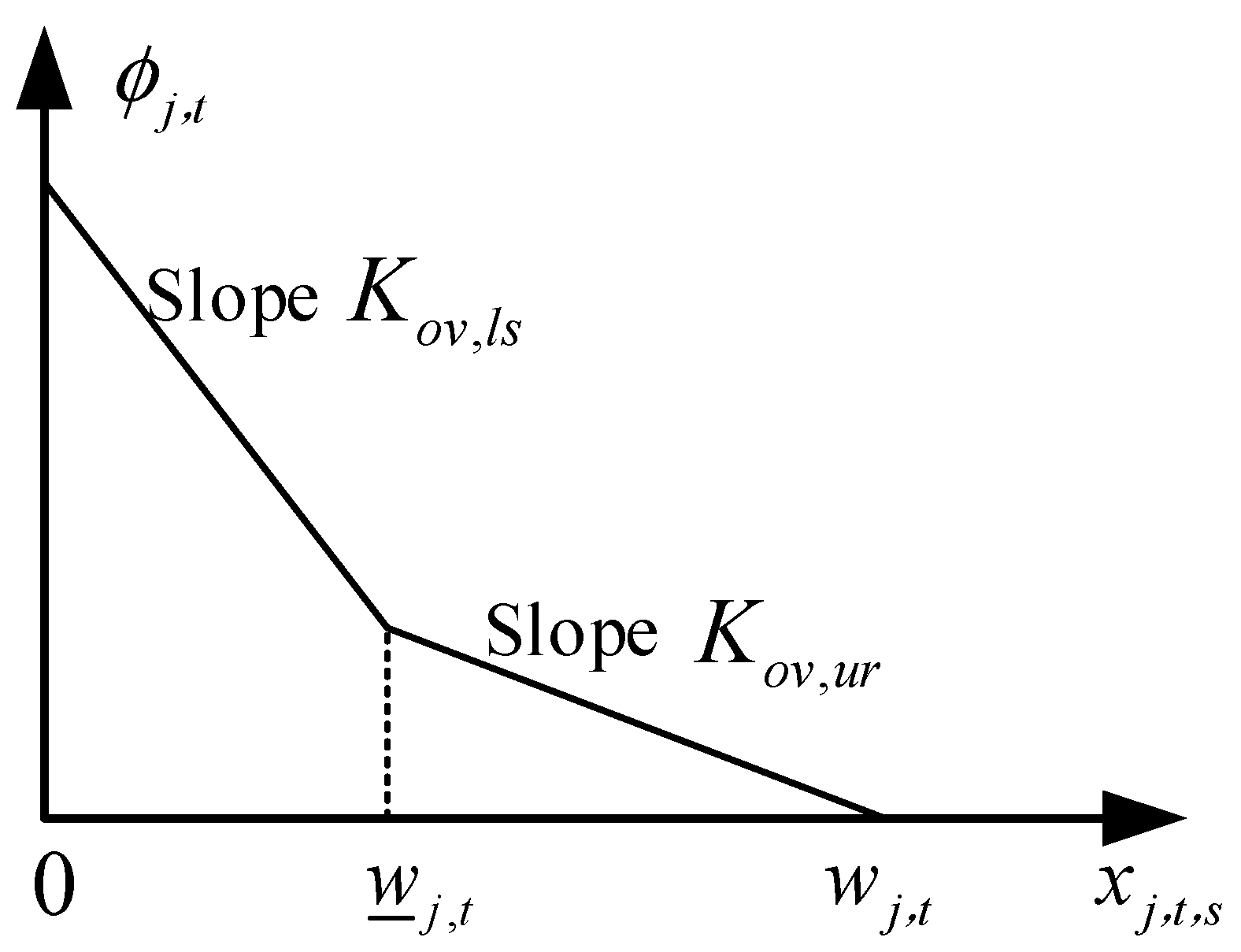
where . is the probability of the s-th segment of discretized probability density function f(x). is the horizontal axis corresponding to the s segment of the probability density function. . is a segmented function, and its function image is shown in Figure 5. The slope of the first segment in Figure 5 is greater than the slope of the second one because the penalty cost for the load shedding is greater than the cost for the upward reserve. Since the objective function is the minimization problem of E, the auxiliary variable can be introduced to convert Equation (33) to Equation (34):
where needs to satisfy the condition shown in Equation (35). Thus, the first two terms in Equation (9) can be expressed by Equations (34) and (35). Similarly, the last two terms in Equation (9) can be expressed by Equations (36) and (37) in which is the corresponding auxiliary variable:
In addition, the decision variables which correspond to the boundaries of 99 different confidence levels are discrete, and a binary variable ICP is introduced to handle them. Set ICP as a 1 × 99 vector, if the 90th element is 1 and the other elements are 0, the confidence level is 90%. Thus, through Equations (38) and (39), the wind power confidence level can be associated with the wind power interval boundaries . That is, the actual decision variable is ICP:
where Wup and Wdn are T × 99 matrices, representing the upper and lower boundaries of wind power intervals with 99 different confidence levels. The calculation method can refer to Section 2.2.
All the nonlinear terms are linearized, and the model established in this paper is converted into a mixed integer linear programming problem (MILP) that can be solved using commercial optimization software CPLEX.
4. Simulation and Discussion
4.1. Data and Parameters Setting
The 10-units system and 118-bus system are tested to verify the effectiveness and superiority of the proposed models. The wind power and load data are shown in Appendix A. The upper and lower limits of the generator output, the minimum start-up and shut-down time, the fuel cost coefficients, the reserve cost coefficients and so on can refer to [6,18]. The wind power data in 2015 and 2016 from [19] is used to simulate the empirical PDF. The capacity of the wind farm is set as 350 MW, and the cost coefficients , , and are 120, 200, 60 and 120 USD/MW, respectively. The simulations are conducted based on Matlab 2013a, and CPLEX 12.6.1.
4.2. Results of UC Model
Simulation of four cases are conducted in this section. Cases 1 and 3 are tested on the 10-units system. Cases 2 and 4 are tested on the 118-bus system. In cases 1 and 2, the confidence levels of the 24 h are set to be the same. In cases 3 and 4, the 24-h wind power confidence levels are different.
4.2.1. Case 1 and Case 2
Table 1 shows the output of conventional units. It can be seen from Table 1 that the output of the units is in accordance with the distribution of the load. Units 1 and 2 are always on because they have the largest capacity and are used to ensure the supply of power to basic load.
The calculated optimal confidence of case 1 is 73%, and the corresponding optimal wind power confidence intervals is shown in Figure 6. The costs are shown in Table 2.
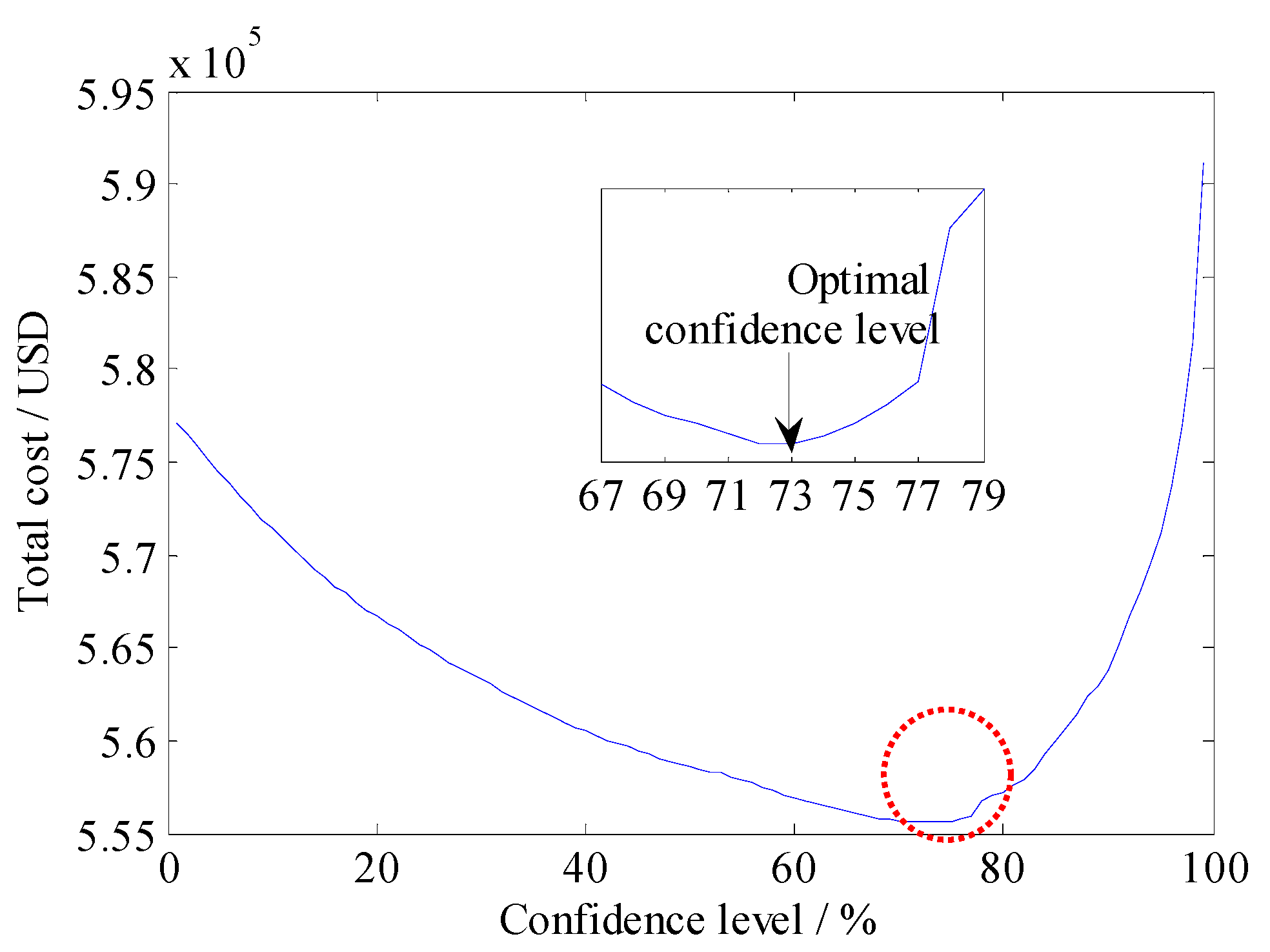
In order to verify the effectiveness of the proposed UC model based on the optimal confidence intervals, the UC model with a specified confidence level is compared with it. The total costs with confidence levels from 1% to 99% is shown in Figure 7.
It can be seen from Figure 7 that the overall cost of the UC model shows a trend of decreasing first and then increasing with the gradual increase of the confidence level. There are few local minimum points in the curve, and it is found that the global minimum point is the confidence level of 73%, which is consistent with the simulation results of the proposed model and proves the effectiveness of the proposed model. In addition, the confidence level of the traditional UC model based on the wind power intervals is usually set to be more than 90%, which will lead an over-conservative scheme, and thereby increase the overall cost of the system.
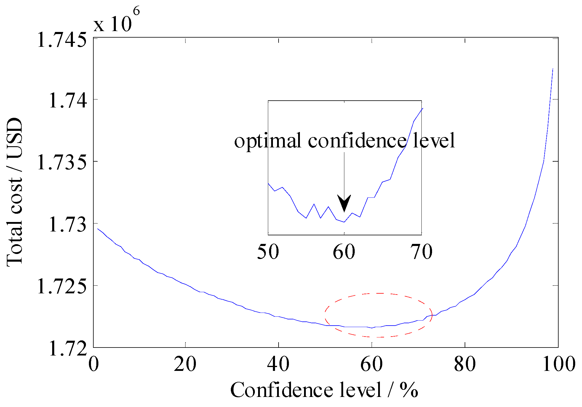
To further verify the effectiveness of the proposed model, the test on 118-bus system is carried out. The optimal confidence level of case 2 is 60% and the costs are shown in Table 2. The total costs under different confidence levels are shown in Figure 8, in which the global minimum point is the confidence level of 60% and it is consistent with the simulation results of the proposed model. Thus, the same conclusions can be drawn.
4.2.2. Case 3 and Case 4
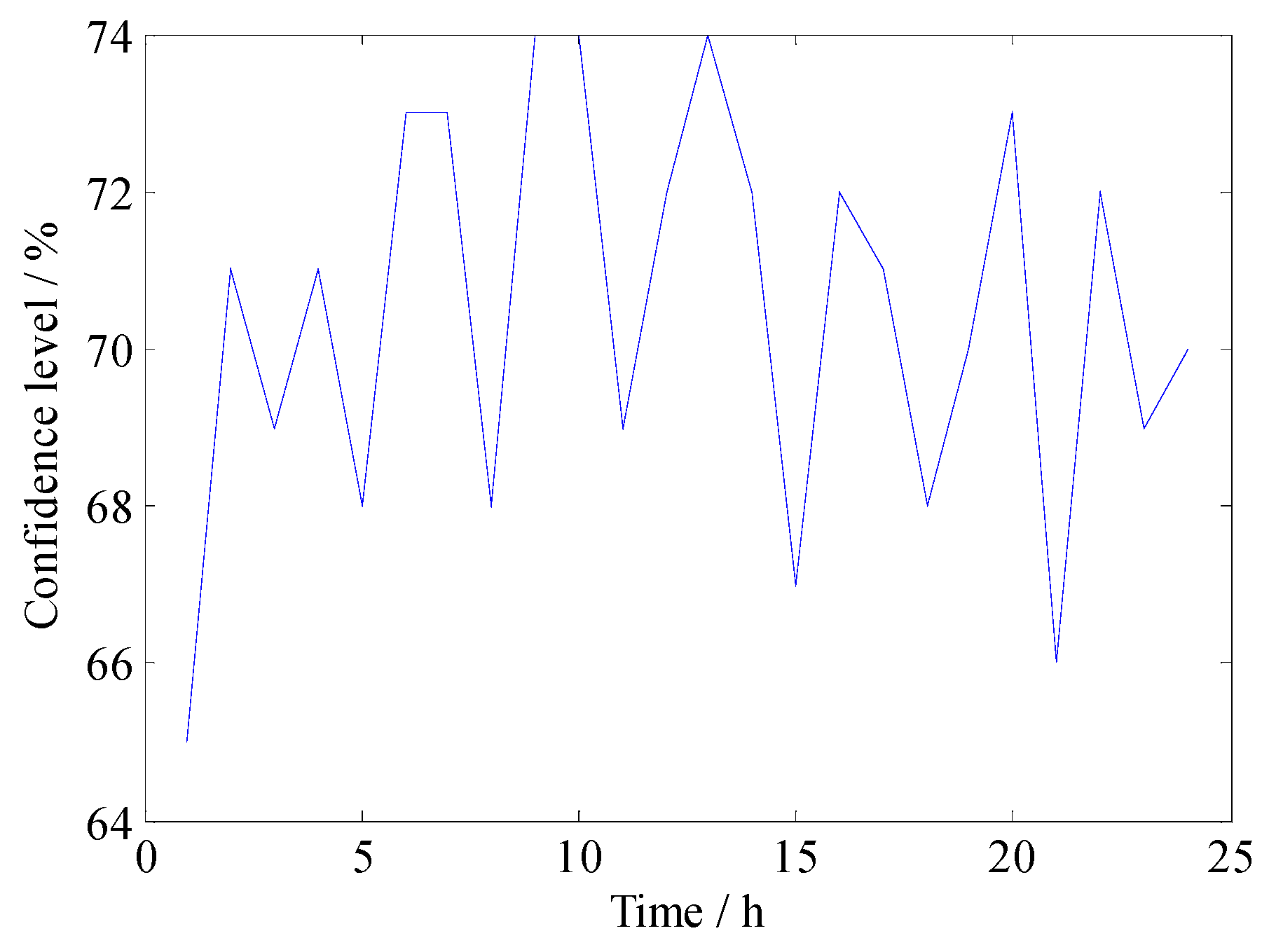
The output results of Case 3 are shown in Table 3. The optimal confidence intervals and optimal confidence levels for Case 3 are shown in Figure 9 and Figure 10.
The costs of Case 3 and Case 4 are shown in Table 4. Compared with Table 2, it can be seen that the total cost of Case 3 is lower than that of Case 1 because Case 3 increases the complexity of the problem on the basis of Case 1, that is, setting the confidence levels for 24 h different from each other, and the solution space is expanded.
In addition, the fuel cost of the thermal power units is 475,488 USD which is less than 491,300 USD of Case 1 and indicates that the overall output of the thermal power units is less than that of the Case 1. Because the scheduled wind power in Case 3 is increased, that is, the capacity of wind power consumption in Case 3 is improved. In conclusion, Case 3 further reduces overall costs and increases the capacity of wind power consumption. Comparing Case 2 and Case 4, the same conclusions can be obtained.
4.3. Rolling Dispatch Model Results
In this section, the rolling plan simulation experiment is carried out on the basis of the day-ahead unit commitment plan. The scheduling time is 4 h. The system parameters and cost coefficients are the same as those in Section 4.2. The values of risk penalty factor and cost coefficient of output regulation can refer to Appendix A.
Three cases are studied in this section. Both Case 5 and Case 6 consider fuel cost, reserve cost, and risk cost, excluding regulation cost. The difference between Case 5 and Case 6 is that the confidence levels in all four periods of Case 5 are limited to more than 90% while in Case 6 this condition is limited only in the first period. Case 7 includes regulation cost on basis of Case 6.
4.3.1. Comparison of Case 5 and Case 6
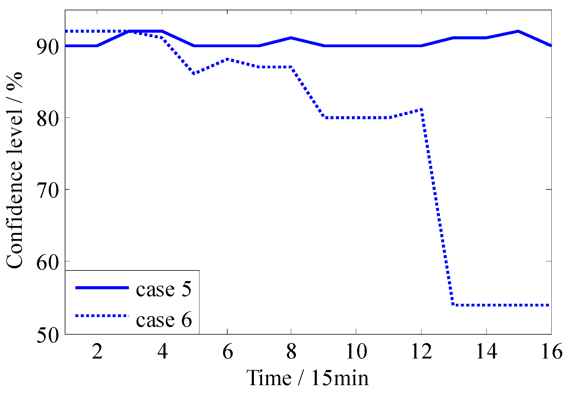
The rolling plan results performed in the 14th to 17th h for Case 5 and Case 6 are shown in Appendix A, corresponding to the outputs of the DI, EI, FI and GI periods in Figure 4. Taking tD–tH periods as an example, when formulating the rolling plan at time , the optimal confidence levels for Case 5 and Case 6 are shown in Figure 11. It can be seen that the confidence levels in 4 h for Case 5 are greater than 90%, and the confidence levels for Case 6 decrease with the time. In order to observe the difference between the results of Case 5 and Case 6, the costs of the actual executed plans for tD–tH periods are shown in Table 5. It can be seen that the total cost of Case 6 is smaller than that of Case 5. The reason for this difference is that Case 5 aims at optimizing the fuel cost and risk cost of each rolling plan, but lacks consideration of the overall optimality within the dispatching periods.
4.3.2. Comparison of Case 6 and Case 7
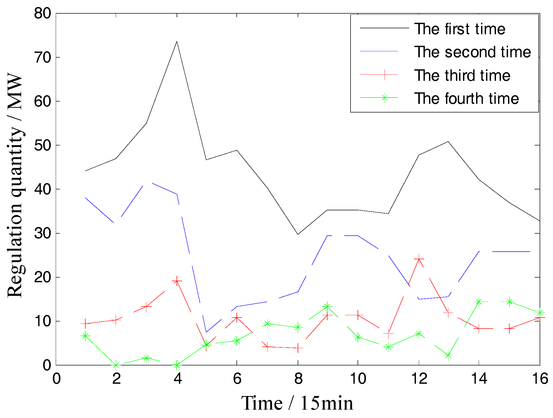
The output regulations for different rolling plans are shown in Figure 12 and Figure 13, in which the quantity of each regulation in Case 7 is greatly reduced compared with that in Case 6.
The first regulation quantity in Figure 13 is greater than the other regulations. This is because the deviation between the day-ahead and intra-day wind power forecast results is larger than that between the intra-day neighboring rolling forecast results, and the regulations are made to correct the deviations. In addition, the regulation quantity is gradually reduced in Case 7, which indicates that the intra-day rolling plans can gradually correct the deviations of day-ahead plan. If all the regulations are executed in advance, it will be difficult and risky. From this perspective, the result of Case 7 is superior to Case 6.
The costs and regulation quantity of Case 6 and Case 7 are shown in Table 6. It can be seen that the regulation quantity of Case 7 is significantly smaller, and the fuel cost is smaller than Case 6. The reason for this difference is that Case 6 lacks consideration of the regulation costs, which leads to repeated regulations among the rolling plans. The lower fuel cost of Case 7 indicates that the total output of thermal power units is less, and thus the wind power output is greater. That is, the capacity of consuming wind power has been improved.
5. Conclusions
A unit commitment model considering the optimal wind power confidence intervals is proposed to balance the economic cost and risk of power system with wind power integration. On the basis, in order to achieve the global optimality of the overall cost, regulation cost is taken into account to establish an intra-day rolling dispatch model based on optimal confidence intervals. Through the simulation of the models, the following conclusions can be drawn:
- (1)
- The simulation results show that as the wind power confidence level changes, there is a tradeoff between the economic cost and risk cost. The global optimal point which balance the economic cost and risk cost of the system can be effectively obtained by the proposed model.
- (2)
- The simulation results of intra-day rolling dispatch model shows that this model can help to reduce the regulation quantity and avoid repeated regulations, thereby reducing the overall cost within the scheduling periods.
Author Contributions
Data curation, M.H.; Methodology, Z.H.; Writing—review & editing, M.H.
Funding
This research received no external funding.
Conflicts of Interest
The authors declare no conflict of interest.
Appendix A

Table A1.
The day-ahead predicted wind power data (p.u.).
| Time Period | 1 | 2 | 3 | 4 | 5 | 6 | 7 | 8 | 9 | 10 | 11 | 12 |
|---|---|---|---|---|---|---|---|---|---|---|---|---|
| Wind power | 0.57 | 0.49 | 0.42 | 0.36 | 0.28 | 0.2 | 0.15 | 0.11 | 0.1 | 0.12 | 0.16 | 0.23 |
| Time period | 13 | 14 | 15 | 16 | 17 | 18 | 19 | 20 | 21 | 22 | 23 | 24 |
| Wind power | 0.32 | 0.43 | 0.52 | 0.59 | 0.68 | 0.74 | 0.68 | 0.64 | 0.57 | 0.49 | 0.41 | 0.33 |
Table A2.
The intra-day rolling predicted wind power data (p.u.).
| Number | Time Period | |||||||||||||||
|---|---|---|---|---|---|---|---|---|---|---|---|---|---|---|---|---|
| 1 | 2 | 3 | 4 | 5 | 6 | 7 | 8 | 9 | 10 | 11 | 12 | 13 | 14 | 15 | 16 | |
| 1 | 0.12 | 0.14 | 0.16 | 0.18 | 0.23 | 0.24 | 0.26 | 0.26 | 0.26 | 0.28 | 0.32 | 0.35 | 0.41 | 0.44 | 0.47 | 0.51 |
| 2 | 0.22 | 0.23 | 0.25 | 0.25 | 0.25 | 0.27 | 0.31 | 0.34 | 0.4 | 0.43 | 0.46 | 0.5 | 0.57 | 0.61 | 0.62 | 0.62 |
| 3 | 0.25 | 0.27 | 0.3 | 0.33 | 0.39 | 0.42 | 0.44 | 0.48 | 0.55 | 0.59 | 0.6 | 0.61 | 0.68 | 0.68 | 0.7 | 0.75 |
| 4 | 0.38 | 0.41 | 0.43 | 0.47 | 0.53 | 0.57 | 0.58 | 0.58 | 0.66 | 0.66 | 0.68 | 0.73 | 0.77 | 0.81 | 0.81 | 0.82 |
| 5 | 0.52 | 0.56 | 0.56 | 0.57 | 0.64 | 0.64 | 0.65 | 0.7 | 0.78 | 0.82 | 0.83 | 0.83 | 0.85 | 0.82 | 0.77 | 0.74 |
| 6 | 0.62 | 0.62 | 0.64 | 0.68 | 0.76 | 0.79 | 0.8 | 0.8 | 0.83 | 0.8 | 0.75 | 0.72 | 0.67 | 0.66 | 0.69 | 0.68 |
| 7 | 0.74 | 0.77 | 0.77 | 0.78 | 0.8 | 0.77 | 0.72 | 0.69 | 0.65 | 0.64 | 0.67 | 0.67 | 0.65 | 0.61 | 0.54 | 0.52 |
Table A3.
The day-ahead predicted load data (MW).
| Time Period | 1 | 2 | 3 | 4 | 5 | 6 | 7 | 8 | 9 | 10 | 11 | 12 |
|---|---|---|---|---|---|---|---|---|---|---|---|---|
| Load | 700 | 750 | 850 | 950 | 1000 | 1100 | 1150 | 1200 | 1300 | 1400 | 1500 | 1550 |
| Time period | 13 | 14 | 15 | 16 | 17 | 18 | 19 | 20 | 21 | 22 | 23 | 24 |
| Load | 1400 | 1300 | 1200 | 1050 | 1000 | 1100 | 1200 | 1400 | 1300 | 1100 | 900 | 800 |
Table A4.
Parameters of rolling dispatch model.
| μ1 | μ2 | μ3 | μ4 | ||||
|---|---|---|---|---|---|---|---|
| 4 | 3 | 2 | 1 | 5 | 1 | 0.5 | 0.1 |
Table A5.
Executed rolling plans for Case 1.
| Period | G1 | G2 | G3 | G4 | G5 | G6 | G7 | G8 | G9 | G10 |
|---|---|---|---|---|---|---|---|---|---|---|
| 1 | 455 | 247.1 | 130 | 130 | 162 | 50.1 | 0 | 0 | 0 | 0 |
| 2 | 455 | 210.2 | 130 | 130 | 162 | 48.8 | 0 | 0 | 0 | 0 |
| 3 | 455 | 270.2 | 60 | 107.5 | 162 | 48.1 | 0 | 0 | 0 | 0 |
| 4 | 455 | 330.2 | 20 | 70 | 144.3 | 43.2 | 0 | 0 | 0 | 0 |
| 5 | 358.4 | 455 | 0 | 0 | 162 | 41.8 | 0 | 0 | 0 | 0 |
| 6 | 314.2 | 455 | 0 | 0 | 162 | 38.1 | 0 | 0 | 0 | 0 |
| 7 | 261.2 | 455 | 0 | 0 | 162 | 44.8 | 0 | 0 | 0 | 0 |
| 8 | 222.2 | 455 | 0 | 0 | 162 | 44.8 | 0 | 0 | 0 | 0 |
| 9 | 168.3 | 455 | 0 | 0 | 162 | 43.1 | 0 | 0 | 0 | 0 |
| 10 | 150 | 451.7 | 0 | 0 | 162 | 42.7 | 0 | 0 | 0 | 0 |
| 11 | 150 | 454.7 | 0 | 0 | 133.6 | 43.1 | 0 | 0 | 0 | 0 |
| 12 | 150 | 455 | 0 | 0 | 73.6 | 74.2 | 0 | 0 | 0 | 0 |
| 13 | 150 | 455 | 0 | 0 | 93.4 | 47.7 | 0 | 0 | 0 | 0 |
| 14 | 150 | 455 | 0 | 0 | 74.4 | 80 | 0 | 0 | 0 | 0 |
| 15 | 150 | 455 | 0 | 0 | 102 | 78.4 | 0 | 0 | 0 | 0 |
| 16 | 154.5 | 455 | 0 | 0 | 162 | 42.9 | 0 | 0 | 0 | 0 |
Table A6.
Executed rolling plans for Case 2.
| Period | G1 | G2 | G3 | G4 | G5 | G6 | G7 | G8 | G9 | G10 |
|---|---|---|---|---|---|---|---|---|---|---|
| 1 | 455 | 455 | 130 | 20 | 43.7 | 70.5 | 0 | 0 | 0 | 0 |
| 2 | 455 | 455 | 107.4 | 20 | 25 | 73.6 | 0 | 0 | 0 | 0 |
| 3 | 455 | 455 | 78.6 | 20 | 25 | 69.2 | 0 | 0 | 0 | 0 |
| 4 | 428.1 | 395 | 70 | 70 | 25 | 74.6 | 0 | 0 | 0 | 0 |
| 5 | 358.4 | 455 | 0 | 0 | 162 | 41.8 | 0 | 0 | 0 | 0 |
| 6 | 314.2 | 455 | 0 | 0 | 162 | 38.1 | 0 | 0 | 0 | 0 |
| 7 | 261.2 | 455 | 0 | 0 | 162 | 44.8 | 0 | 0 | 0 | 0 |
| 8 | 222.2 | 455 | 0 | 0 | 162 | 44.8 | 0 | 0 | 0 | 0 |
| 9 | 168.3 | 455 | 0 | 0 | 162 | 43.1 | 0 | 0 | 0 | 0 |
| 10 | 150 | 451.7 | 0 | 0 | 162 | 42.7 | 0 | 0 | 0 | 0 |
| 11 | 150 | 427.1 | 0 | 0 | 133.6 | 70.7 | 0 | 0 | 0 | 0 |
| 12 | 150 | 455 | 0 | 0 | 73.6 | 74.2 | 0 | 0 | 0 | 0 |
| 13 | 455 | 200.7 | 0 | 0 | 25 | 65.5 | 0 | 0 | 0 | 0 |
| 14 | 455 | 199 | 0 | 0 | 25.4 | 80 | 0 | 0 | 0 | 0 |
| 15 | 455 | 225 | 0 | 0 | 25.4 | 80 | 0 | 0 | 0 | 0 |
| 16 | 455 | 254 | 0 | 0 | 25.4 | 80 | 0 | 0 | 0 | 0 |
References
- Zavala, E.M.V.M.; Rocklin, M. A computational framework for uncertainty quantification and stochastic optimization in unit commitment with wind power generation. IEEE Trans. Power Syst. 2011, 26, 431–441. [Google Scholar]
- Qianfan, W.; Yongpei, G.; Jianhui, W. A chance-constrained two-stage stochastic program for unit commitment with uncertain wind power output. IEEE Trans. Power Syst. 2012, 27, 206–215. [Google Scholar]
- Lorca, Á.; Sun, X.A. Adaptive robust optimization with dynamic uncertainty sets for multi-period economic dispatch under significant wind. IEEE Trans. Power Syst. 2015, 30, 1702–1713. [Google Scholar] [CrossRef]
- Yu, Y.; Luh, P.B.; Litvinov, E. Grid integration of distributed wind generation: Hybrid markovian and interval unit commitment. IEEE Trans. Smart Grid 2015, 6, 3061–3072. [Google Scholar] [CrossRef]
- Wu, W.; Chen, J.; Zhang, B. A robust wind power optimization method for look-ahead power dispatch. IEEE Trans. Sustain. Energy 2014, 5, 507–515. [Google Scholar] [CrossRef]
- Doostizadeh, M.; Aminifar, F.; Ghasemi, H. Energy and reserve scheduling under wind power uncertainty: An adjustable interval approach. IEEE Trans. Smart Grid 2016, 7, 2943–2952. [Google Scholar] [CrossRef]
- Liu, Y.; Nair, N.C. A two-stage stochastic dynamic economic dispatch model considering wind uncertainty. IEEE Trans. Sustain. Energy 2016, 7, 819–829. [Google Scholar] [CrossRef]
- Ding, T.; Guo, Q.L.; Bo, R. Interval economic dispatch model with uncertain wind power injection and spatial branch and bound method. Proc. CSEE 2014, 34, 3707–3714. [Google Scholar]
- Mei, S.; Zhang, D.; Wang, Y. Robust optimization of static reserve planning with large-scale integration of wind power: A game theoretic approach. IEEE Trans. Sustain. Energy 2014, 5, 535–545. [Google Scholar] [CrossRef]
- Du, E.; Zhang, N.; Kang, C. Exploring the flexibility of CSP for wind power integration using interval optimization. In Proceedings of the IEEE Power and Energy Society General Meeting PESGM, Boston, MA, USA, 17–21 July 2016. [Google Scholar]
- Wang, Y.; Xia, Q.; Kang, C. Unit commitment with volatile node injections by using interval optimization. IEEE Trans. Power Syst. 2011, 26, 1705–1713. [Google Scholar] [CrossRef]
- Wu, L.; Shahidehpour, M.; Li, Z. Comparison of scenario-based and interval optimization approaches to stochastic SCUC. IEEE Trans. Power Syst. 2012, 27, 913–921. [Google Scholar] [CrossRef]
- Li, Z.; Wu, W.; Zhang, B. Robust look-ahead power dispatch with adjustable conservativeness accommodating significant wind power integration. IEEE Trans. Sustain. Energy 2015, 6, 781–790. [Google Scholar] [CrossRef]
- Tang, C.; Xu, J.; Sun, Y. Look-ahead economic dispatch with adjustable confidence interval based on a truncated versatile distribution model for wind power. IEEE Trans. Power Syst. 2017, 33, 1755–1767. [Google Scholar] [CrossRef]
- Xie, L.; Carvalho, P.M.S.; Ferreira, L.A.F.M. Wind integration in power systems: Operational challenges and possible solutions. Proc. IEEE 2011, 99, 214–232. [Google Scholar] [CrossRef]
- Xu, T.; Zhang, N. Coordinated operation of concentrated solar power and wind resources for the provision of energy and reserve services. IEEE Trans. Power Syst. 2017, 32, 1260–1271. [Google Scholar] [CrossRef]
- Ma, X.Y.; Sun, Y.Z.; Fang, H.L. Scenario generation of wind power based on statistical uncertainty and variability. IEEE Trans. Sustain. Energy 2013, 4, 894–904. [Google Scholar] [CrossRef]
- Basu, M. Dynamic economic emission dispatch using nondominated sorting genetic algorithm-II. Int. J. Electr. Power Energy Syst. 2008, 30, 140–149. [Google Scholar] [CrossRef]
- EirGrid, Actual and Forecast Wind Power Data. Available online: http://www.eirgridgroup.com/ (accessed on 15 January 2017).
Figure 1.
Diagram representation of the overview framework.

Figure 2.
Wind power probability density function and confidence interval.
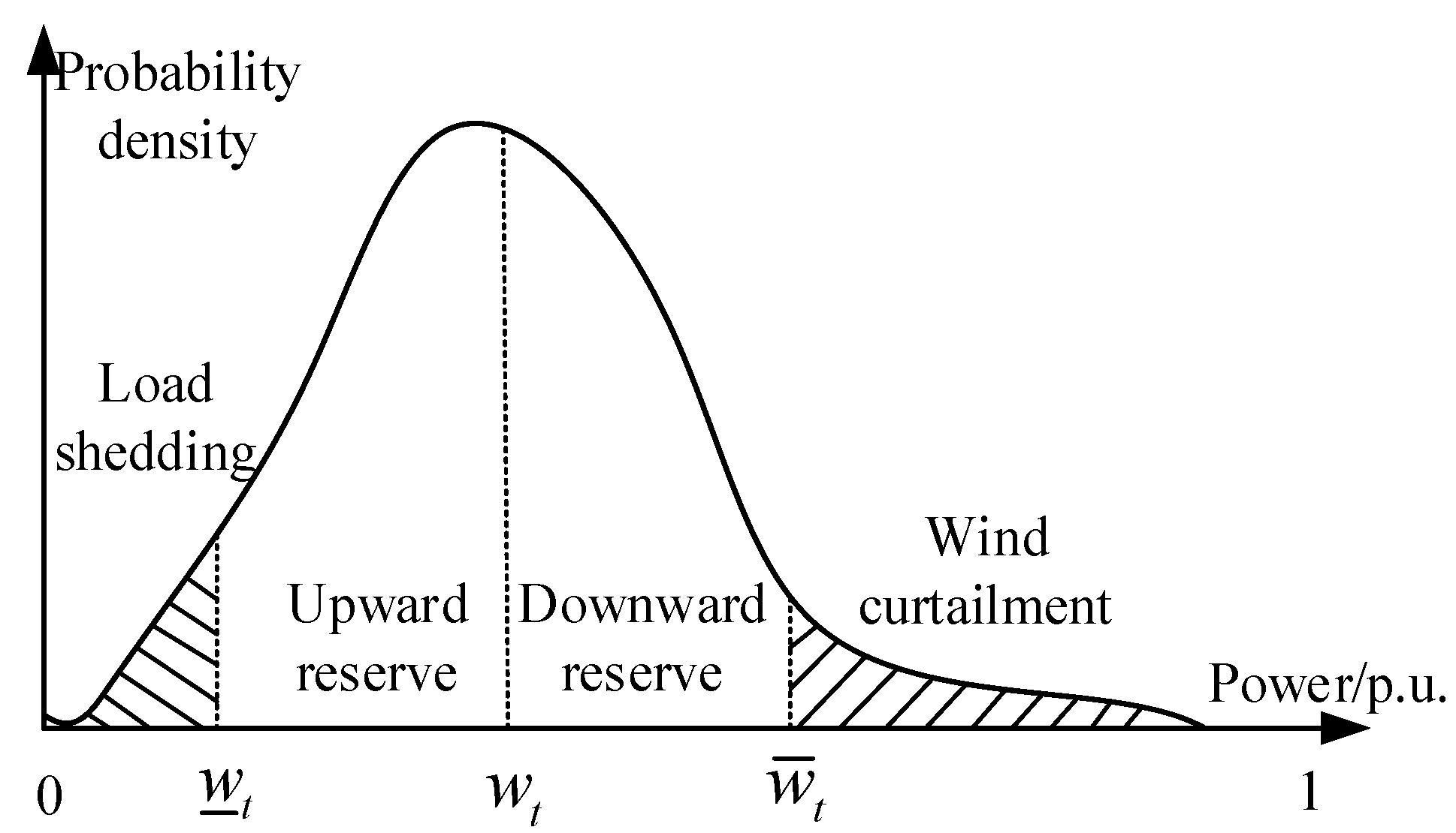
Figure 3.
Schematic diagram of ramp constraints within confidence intervals.
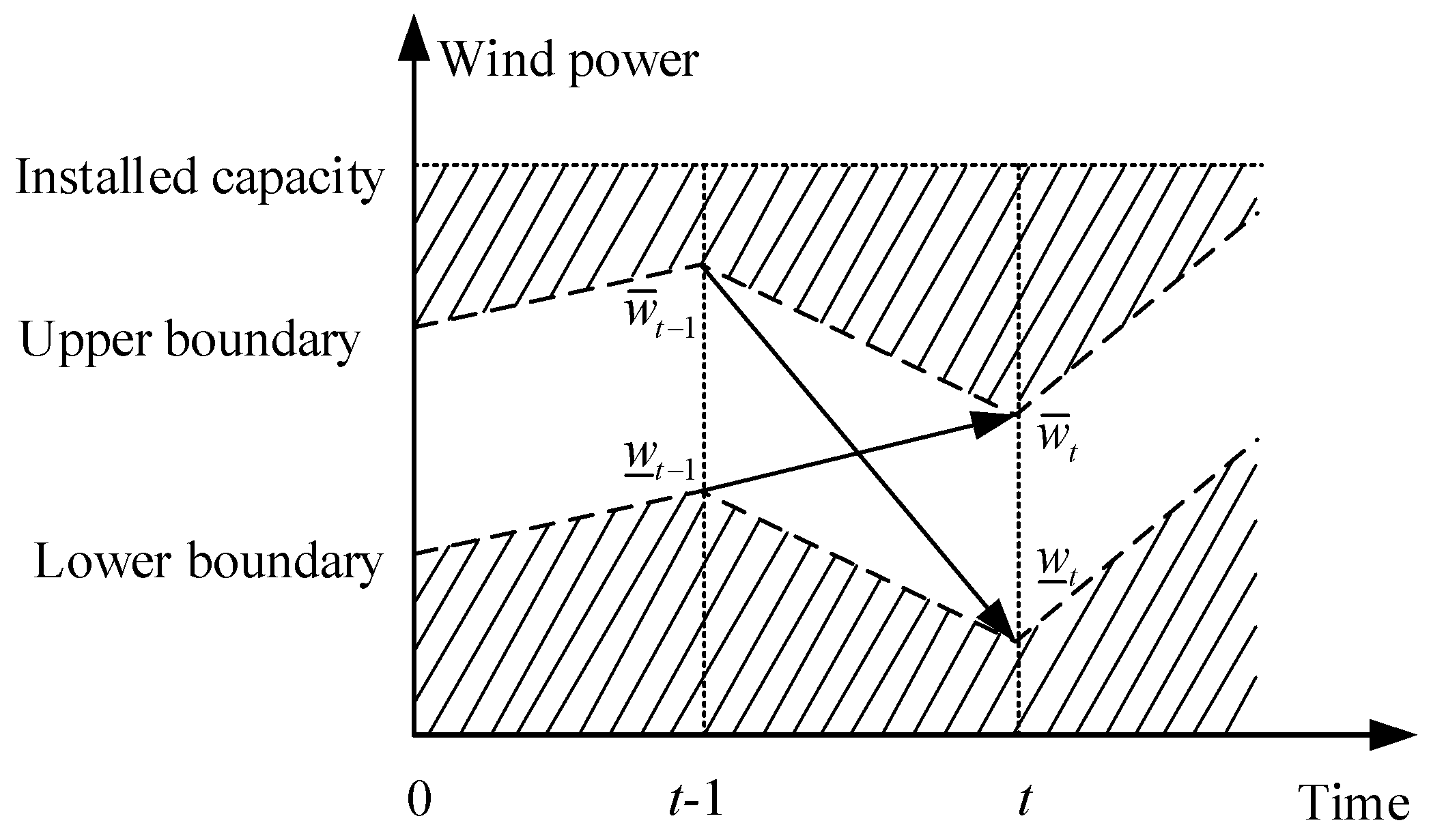
Figure 4.
Overview of the intra-day rolling dispatch.

Figure 5.
Function image of ϕi,t.

Figure 6.
Optimal wind power confidence intervals (Case 1).
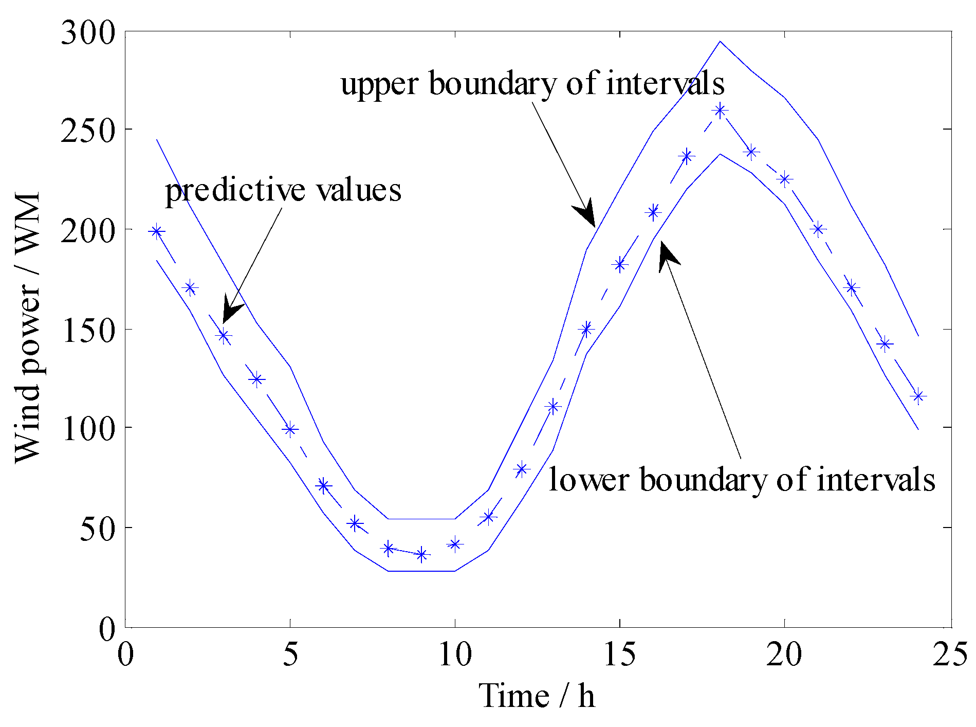
Figure 7.
Total cost under different confidence levels for 10-units system (Case 1).

Figure 8.
Total cost under different confidence levels for 118-bus system (Case 2).

Figure 9.
The optimal wind power confidence levels (Case 3).

Figure 10.
The optimal wind power confidence intervals (Case 3).
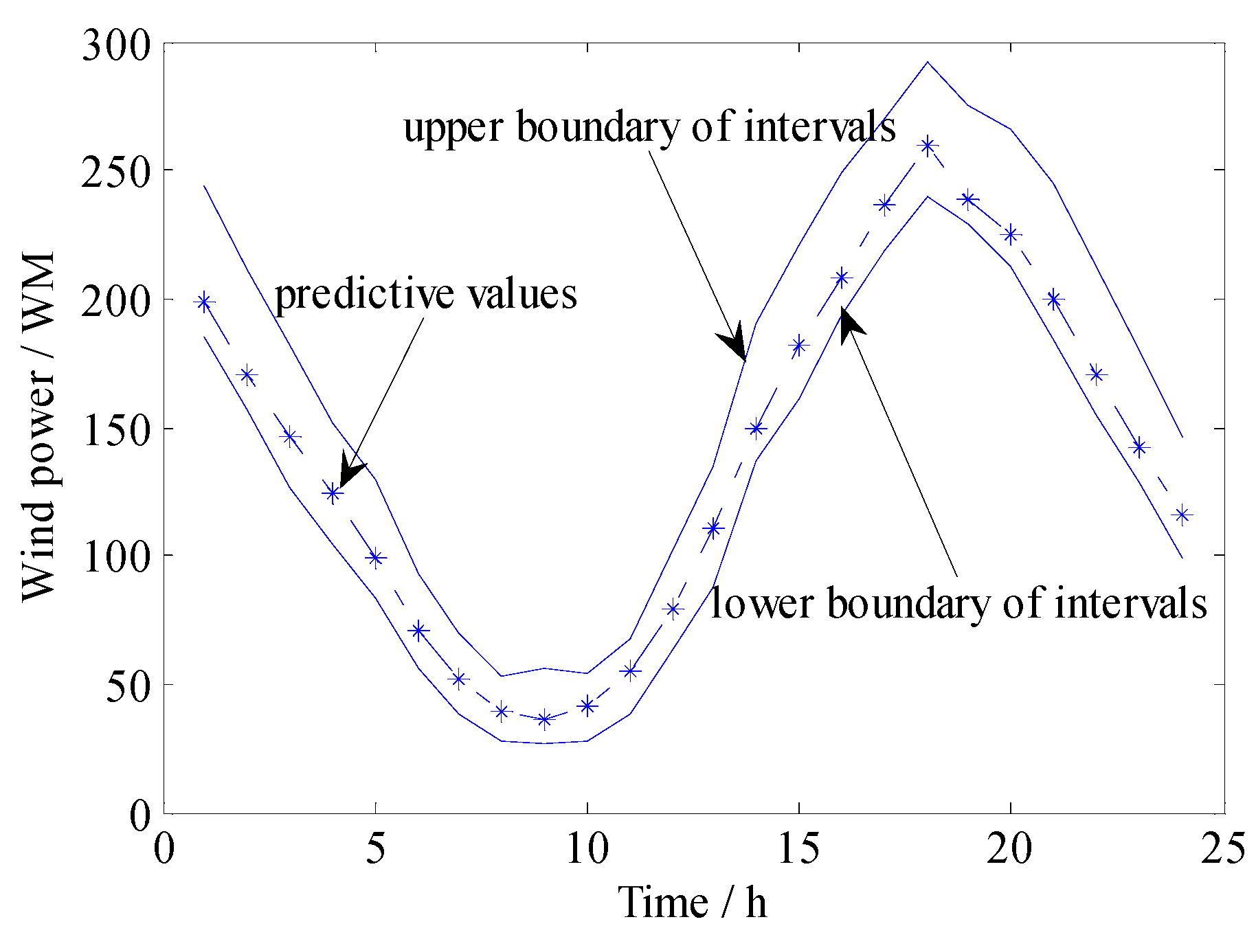
Figure 11.
The optimal wind power confidence levels.

Figure 12.
The output regulations for each period (Case 6).
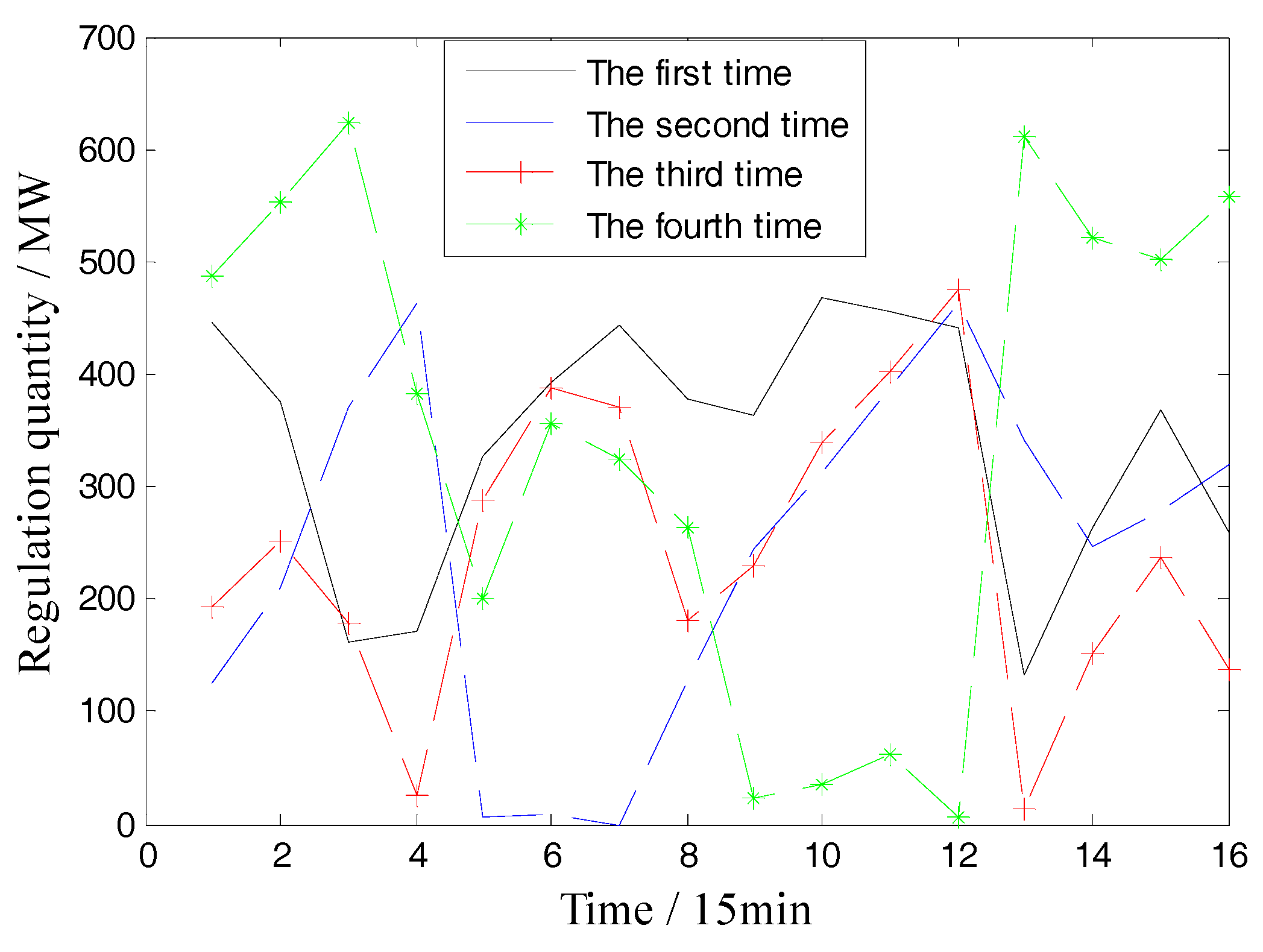
Figure 13.
The output regulations for each period (Case 7).

Table 1.
Conventional units output (Case 1).
| Hour | G1 | G2 | G3 | G4 | G5 | G6 | G7 | G8 | G9 | G10 |
|---|---|---|---|---|---|---|---|---|---|---|
| 1 | 285.7 | 150 | 0 | 0 | 0 | 57.1 | 0 | 0 | 0 | 0 |
| 2 | 316.3 | 202.7 | 0 | 0 | 0 | 49.5 | 0 | 0 | 0 | 0 |
| 3 | 385.5 | 262.7 | 0 | 0 | 0 | 53.1 | 0 | 0 | 0 | 0 |
| 4 | 455 | 322.7 | 0 | 0 | 0 | 51 | 0 | 0 | 0 | 0 |
| 5 | 446.6 | 382.4 | 0 | 20 | 0 | 49.6 | 0 | 0 | 0 | 0 |
| 6 | 455 | 442.4 | 0 | 90 | 0 | 39.9 | 0 | 0 | 0 | 0 |
| 7 | 455 | 455 | 0 | 130 | 0 | 60.8 | 0 | 0 | 0 | 0 |
| 8 | 455 | 455 | 20 | 130 | 25 | 79.2 | 0 | 0 | 0 | 0 |
| 9 | 455 | 455 | 90 | 130 | 85 | 49.2 | 0 | 0 | 0 | 0 |
| 10 | 455 | 455 | 130 | 130 | 145 | 49.2 | 0 | 0 | 0 | 0 |
| 11 | 455 | 455 | 130 | 130 | 162 | 43.8 | 25 | 0 | 0 | 0 |
| 12 | 455 | 455 | 130 | 130 | 162 | 64.4 | 75.1 | 0 | 0 | 0 |
| 13 | 455 | 455 | 90 | 90 | 130.8 | 48.3 | 25 | 0 | 0 | 0 |
| 14 | 455 | 455 | 20 | 20 | 140.4 | 53 | 0 | 0 | 0 | 0 |
| 15 | 455 | 424.6 | 0 | 0 | 80.4 | 53.1 | 0 | 0 | 0 | 0 |
| 16 | 391.5 | 364.6 | 0 | 0 | 25 | 53.3 | 0 | 0 | 0 | 0 |
| 17 | 381.3 | 304.6 | 0 | 0 | 25 | 49.9 | 0 | 0 | 0 | 0 |
| 18 | 408.8 | 335 | 0 | 0 | 42 | 55.8 | 0 | 0 | 0 | 0 |
| 19 | 403.8 | 395 | 0 | 0 | 102 | 54.4 | 0 | 0 | 0 | 0 |
| 20 | 455 | 455 | 0 | 0 | 162 | 80 | 0 | 10 | 0 | 0 |
| 21 | 455 | 455 | 0 | 0 | 115.7 | 57.1 | 0 | 10 | 0 | 0 |
| 22 | 408.2 | 395 | 0 | 0 | 65.8 | 49.5 | 0 | 0 | 0 | 0 |
| 23 | 338.2 | 335 | 0 | 0 | 25 | 53.1 | 0 | 0 | 0 | 0 |
| 24 | 358.4 | 275 | 0 | 0 | 0 | 52.3 | 0 | 0 | 0 | 0 |
Table 2.
The costs for Case 1 and Case 2.
| Case | Total Cost (USD) | Fuel Cost (USD) | Reserve Capacity Cost (USD) | Risk Cost (USD) |
|---|---|---|---|---|
| 1 | 555,574 | 491,300 | 19,158 | 40,516 |
| 2 | 1,721,658 | 1,664,158 | 12,275 | 44,421 |
Table 3.
Conventional units output (Case 3).
| Hour | G1 | G2 | G3 | G4 | G5 | G6 | G7 | G8 | G9 | G10 |
|---|---|---|---|---|---|---|---|---|---|---|
| 1 | 285.6 | 150 | 0 | 0 | 0 | 20 | 0 | 0 | 0 | 0 |
| 2 | 317.1 | 199.4 | 0 | 0 | 0 | 20 | 0 | 0 | 0 | 0 |
| 3 | 387 | 259.4 | 0 | 0 | 0 | 20 | 0 | 0 | 0 | 0 |
| 4 | 454.9 | 319.4 | 0 | 0 | 0 | 20 | 0 | 0 | 0 | 0 |
| 5 | 448.7 | 379.4 | 0 | 20 | 0 | 20 | 0 | 0 | 0 | 0 |
| 6 | 455 | 439.4 | 0 | 90 | 0 | 20 | 0 | 0 | 0 | 0 |
| 7 | 455 | 455 | 0 | 130 | 0 | 36.8 | 0 | 0 | 0 | 0 |
| 8 | 455 | 455 | 20 | 130 | 25 | 59.8 | 0 | 0 | 0 | 0 |
| 9 | 455 | 455 | 90 | 130 | 85 | 27.3 | 0 | 0 | 0 | 0 |
| 10 | 455 | 455 | 130 | 130 | 145 | 27.3 | 0 | 0 | 0 | 0 |
| 11 | 455 | 455 | 130 | 130 | 162 | 72.3 | 25 | 0 | 0 | 0 |
| 12 | 455 | 455 | 130 | 130 | 162 | 34.7 | 77 | 0 | 0 | 0 |
| 13 | 455 | 455 | 90 | 90 | 125.4 | 20 | 25 | 0 | 0 | 0 |
| 14 | 455 | 455 | 20 | 20 | 136.7 | 20 | 0 | 0 | 0 | 0 |
| 15 | 455 | 427.9 | 0 | 0 | 76.7 | 20 | 0 | 0 | 0 | 0 |
| 16 | 386.3 | 367.9 | 0 | 0 | 25 | 20 | 0 | 0 | 0 | 0 |
| 17 | 374.4 | 307.9 | 0 | 0 | 25 | 20 | 0 | 0 | 0 | 0 |
| 18 | 422.6 | 335 | 0 | 0 | 26.8 | 20 | 0 | 0 | 0 | 0 |
| 19 | 416.6 | 395 | 0 | 0 | 86.8 | 20 | 0 | 0 | 0 | 0 |
| 20 | 455 | 455 | 0 | 0 | 146.8 | 61.7 | 0 | 10 | 0 | 0 |
| 21 | 455 | 455 | 0 | 0 | 115.3 | 20 | 0 | 10 | 0 | 0 |
| 22 | 406.5 | 395 | 0 | 0 | 64.9 | 20 | 0 | 0 | 0 | 0 |
| 23 | 336.5 | 335 | 0 | 0 | 25 | 20 | 0 | 0 | 0 | 0 |
| 24 | 356.4 | 275 | 0 | 0 | 0 | 20 | 0 | 0 | 0 | 0 |
Table 4.
The costs for Case 3 and Case 4.
| Case | Total Cost (USD) | Fuel Cost (USD) | Reserve Capacity Cost (USD) | Risk Cost (USD) |
|---|---|---|---|---|
| 3 | 541,554 | 475,488 | 21,365 | 40,101 |
| 4 | 1,720,576 | 1,663,199 | 12,461 | 44,112 |
Table 5.
Comparison of simulation results for Case 5 and Case 6.
| Case | Total Cost (USD) | Fuel Cost (USD) | Upward Reserve Cost (USD) | Downward Reserve Cost (USD) | Risk Cost (USD) |
|---|---|---|---|---|---|
| 5 | 423,525 | 364,359 | 10,749.4 | 18,800.6 | 29,616 |
| 6 | 421,114.3 | 361,927.3 | 12,713.8 | 16,836.2 | 29,637 |
Table 6.
Comparison of simulation results for Case 6 and Case 7.
| Case | Regulation 1 (MW) | Regulation 2 (MW) | Regulation 3 (MW) | Regulation 4 (MW) | Fuel Cost (USD) | Risk Cost (USD) | Reserve Cost (USD) |
|---|---|---|---|---|---|---|---|
| 6 | 6727.2 | 1574.5 | 1987.5 | 2363.3 | 361927.3 | 29637 | 29550 |
| 7 | 699.4 | 392.3 | 166.8 | 109.4 | 359407.1 | 29819 | 28739.6 |
© 2018 by the authors. Licensee MDPI, Basel, Switzerland. This article is an open access article distributed under the terms and conditions of the Creative Commons Attribution (CC BY) license (http://creativecommons.org/licenses/by/4.0/).
Share and Cite
MDPI and ACS Style
Hu, M.; Hu, Z. Optimization Scheduling Method for Power Systems Considering Optimal Wind Power Intervals. Energies 2018, 11, 1710. https://doi.org/10.3390/en11071710
AMA Style
Hu M, Hu Z. Optimization Scheduling Method for Power Systems Considering Optimal Wind Power Intervals. Energies. 2018; 11(7):1710. https://doi.org/10.3390/en11071710
Chicago/Turabian StyleHu, Mengyue, and Zhijian Hu. 2018. "Optimization Scheduling Method for Power Systems Considering Optimal Wind Power Intervals" Energies 11, no. 7: 1710. https://doi.org/10.3390/en11071710
Note that from the first issue of 2016, this journal uses article numbers instead of page numbers. See further details here.