Article

Solving Non-Smooth Optimal Power Flow Problems Using a Developed Grey Wolf Optimizer

1
Department of Electrical Engineering, Faculty of Engineering, Aswan University, Aswan 81542, Egypt
2
State Key Laboratory of Power Transmission Equipment and System Security and New Technology, Chongqing University, Chongqing 400030, China
3
Department of Electrical Engineering, Faculty of Engineering, Sohag University, Sohag 82524, Egypt
4
Department of Electrical Engineering, University of Jaén, EPS Linares, 23700 Jaén, Spain
*
Author to whom correspondence should be addressed.
Energies 2018, 11(7), 1692; https://doi.org/10.3390/en11071692
Submission received: 13 June 2018 / Revised: 25 June 2018 / Accepted: 26 June 2018 / Published: 28 June 2018
(This article belongs to the Special Issue Optimization Methods Applied to Power Systems)

Abstract

:
The optimal power flow (OPF) problem is a non-linear and non-smooth optimization problem. OPF problem is a complicated optimization problem, especially when considering the system constraints. This paper proposes a new enhanced version for the grey wolf optimization technique called Developed Grey Wolf Optimizer (DGWO) to solve the optimal power flow (OPF) problem by an efficient way. Although the GWO is an efficient technique, it may be prone to stagnate at local optima for some cases due to the insufficient diversity of wolves, hence the DGWO algorithm is proposed for improving the search capabilities of this optimizer. The DGWO is based on enhancing the exploration process by applying a random mutation to increase the diversity of population, while an exploitation process is enhanced by updating the position of populations in spiral path around the best solution. An adaptive operator is employed in DGWO to find a balance between the exploration and exploitation phases during the iterative process. The considered objective functions are quadratic fuel cost minimization, piecewise quadratic cost minimization, and quadratic fuel cost minimization considering the valve point effect. The DGWO is validated using the standard IEEE 30-bus test system. The obtained results showed the effectiveness and superiority of DGWO for solving the OPF problem compared with the other well-known meta-heuristic techniques.

1. Introduction

Recently, OPF problems have become a strenuous task for optimal operation of the power systems. The main objective of OPF is finding the best operation, security and economic settings of electrical power systems. In this study, the operating variables of systems are determined optimally for different objective functions such as fuel cost minimization, power loss minimization, emission and voltage deviation minimization, etc., while in addition, enhancing system stability, loadability and voltage profiles. Practically, the solution of OPF problem must satisfy the equality and inequality system constraints [1,2].
OPF is a non-smooth and non-linear optimization problem that is considered a complicated problem. This problem becomes especially more difficult when the equality and inequality operating system constraints are considered. Thus, solving the OPF problem needs more efficient and developed meta-heuristic optimization algorithms. Many conventional methods have been developed in order to solve the OPF problem such as NLP [3], LP [4], QP [5], Newton’s Method [6], IP [7]. However, these methods face some problems in solving nonlinear or non-convex objective functions. In addition, these methods may fall into local minima, hence new optimization algorithms have been proposed to avoid the shortcomings of these methods. From these methods; GA [8,9], MFO [10], DE [11,12], PSO [13], MSA [14], EP [15,16], ABC [17], GSA [18], BBO [19], SFLA [20], forced initialized differential evolution algorithm [21], TS [22], MDE [23], SOS [24], BSA [25] and TLBO [26], decentralized decision-making algorithm [27]. The thermal generation units have multiple valves to control the output generated power. As the valves of thermal generation units are opened in case of steam admission, a sudden increase in losses is observed which leads to ripples in the cost function curve (known as the valve-point loading effect). Several optimization techniques have been employed for solving the OPF considering the valve-point loading effect such as ABC [17], GSA [18], SFLA [20], SOS [24], BSA [25] and Hybrid Particle Swarm Optimization and Differential Evolution [28].
The conventional and some meta-heuristics methods could not efficiently solve the OPF problem, thus several new or modified versions of optimization techniques have been proposed. The GWO algorithm is considered a new optimization technique that proposed by Mirjalili [29]. GWO simulates the grey wolves’ social hierarchy and hunting behavior. The main phases of gray wolf hunting are the approaching, encircling and attacking the prey by the grey wolves [29,30]. It should point out that the conventional GWO technique updates its hunters towards the prey based on the condition of leader wolves. However, the population of GWO is still inclined to stall in local optima in some cases. In addition, the GWO technique is not capable of performing a seamless transition from the exploration to exploitation phases. In this paper, a new developed version of GWO is proposed to effectively solve the OPF problem. The DGWO is based on enhancing the exploration phase by applying a random mutation in order to enhance the searching process and avoid the stagnation at local optima. The exploitation process is improved by updating the populations of GWO in spiral path around the best solution to focus on the most promising regions. DGWO is applied for minimizing the quadratic fuel cost, fuel cost considering the valve loading. The obtained simulation results by the DGWO are compared with those obtained by the classical GWO and other well-known techniques to demonstrate the effectiveness of the proposed algorithm.
The rest of paper is organized as follows: Section 2 presents the optimal power flow problem formulation. Section 3 presents the mathematical formulation of GWO and DGWO techniques. Section 4 presents the numerical results. Finally, the conclusions presented in Section 5.

2. Optimal Power Flow Formulation

Solution of OPF problem aims to achieve certain objective functions by adjustment some control variables with satisfying different operating constraints. Generally, the optimization problem can be mathematically represented as:
M i n F ( x , u )
Subject to:
g j ( x , u ) = 0 j = 1 , 2 , , m
h j ( x , u ) 0 j = 1 , 2 , , p
where, F is a certain objective function, x are the state variables, u is the control variables vector, g j and h j are equality and inequality operating constraints, respectively. m and p are the number of the equality and inequality operating constraints, respectively. The state variables vector (x) can be given as:
x = [ P G 1 , V L 1 V L N P Q , Q G 1 Q G N P V , S T L 1 S T L N T L ]
where, P G 1 is the generated power of slack bus, V L is the load bus voltage, Q G is the generated reactive power, S T L is the power flow in the line, N P Q is the load buses number, N P V is the generated buses number and N T L is the lines number. The independent variables u can be given as:
u = [ P G 2 P G N G , V G 1 V G N G , Q C 1 Q C N C , T 1 T N T ]
where, P G is the generated active power, V G is the generated voltage, Q C is the shunt compensator injected reactive power, T is the transformer tap setting, N G is the generators number, N C is the shunt compensator units and N T is the transformers number.

2.1. Objective Functions

2.1.1. Quadratic Fuel Cost

The first objective function is the quadratic equation of total generation fuel cost which formulated as follows:
F 1 = i = 1 N P V F i ( P G i ) = i = 1 N P V ( a i + b i P G i + c i P G i 2 )
where, F i is the fuel cost. a i , b i and c i are the cost coefficients.

2.1.2. Quadratic Cost with Valve-Point Effect and Prohibited Zones

Practically, the effect of valve point loading for thermal power plants should be considered. This effect occurred as a result of the rippling influence on the unit’s cost curve which produced from each steam admission in the turbine as shown in Figure 1.
The valve point loading effect is considered by adding a sine term to the fuel cost as:
F ( x , u ) = i = 1 N P V F i ( P G i ) = i = 1 N P V ( a i + b i P G i + c i P 2 G i ) + | d i sin ( e i ( P G i m i n P G i ) ) |
where, d i and e i are the fuel cost coefficients considering the valve-point effects.

2.1.3. Piecewise Quadratic Cost Functions

Due to the different fuel sources (coal, natural gas and oil), their fuel cost functions can be considered as a non-convex problem which is given as:
F ( P G i ) = { a i 1 + b i 1 P G i + c i 1 P G i 2 P G i m i n P G i P G 1 a i 2 + b i P G i + c i P G i 2 P G 1 P G i P G 2 a i k + b i k P G i + c i k P G i 2 P G i   k 1 P G i P G i m a x
where, a i k , b i k and c i k are cost coefficients of the ith generator for fuel type k.

2.2. Operating Constraints

2.2.1. Equality Operating Constraints

The operating equality constrains can be represented as:
P G i P D i = | V i | j = 1 N B | V j | ( G i j cos δ i j + B i j sin δ i j )
Q G i Q D i = | V i | j = 1 N B | V j | ( G i j cos δ i j + B i j sin δ i j )
where, P G i and Q G i are the generated power at bus i. P D i and Q D i are load demand at bus i. G i j and B i j are the real and imaginary parts of admittance between bus i and bus j, respectively.

2.2.2. Inequality Operating Constrains

The inequality operating constrains can be given as:
P G i m i n P G i P G i m a x i = 1 , 2 , ,   N G
V G i m i n V G i V G i m a x i = 1 , 2 , ,   N G
Q G i m i n Q G i Q G i m a x i = 1 , 2 , ,   N G
T i m i n T i T i m a x i = 1 , 2 , ,   N T
Q C i m i n Q C i Q C i m a x i = 1 , 2 , ,   N C
S L i S L i m i n i = 1 , 2 , ,   N T L
V L i m i n V L i V L i m a x i = 1 , 2 , ,   N P Q
where, P G i m i n and P G i m a x are the minimum and maximum generated active power limits of ith generator, respectively. V G i m i n and V G i m a x are the lower and upper output voltage limits of ith generator, respectively. Q G i m i n and Q G i m a x are the minimum and maximum generated reactive power limits of ith generator, respectively. T i m i n and T i m a x are the lower and upper limits of regulating transformer i. Q C i m i n and Q C i m a x are the minimum and maximum injected VAR of ith shunt compensation unit. S L i is the apparent power flow in ith line while S L i m i n is the maximum apparent power flow of this line. V L i m i n and V L i m a x are the lower and upper limits of voltage magnitude load bus i, respectively.
The dependent state variables can be considered in OPF solution using the quadratic penalty formulation as:
F g ( x , u ) = F i ( x , u ) + K G ( P G 1 P G 1 l i m ) 2 + K Q i = 1 N P V ( Q G i Q G i l i m ) 2 + K V i = 1 N P Q ( V L i V L i l i m ) 2 + K S i = 1 N T L ( S L i S L i l i m ) 2
where, K G , K Q , K V , K S and K S are the penalty factors. x l i m is the limit value that can be given as:
x l i m = { x m a x ; x > x m a x x m i n ; x < x m i n
where, x m a x and x m i n are the upper and lower limits of the dependent variables, respectively.

3. Developed Grey Wolf Optimizer

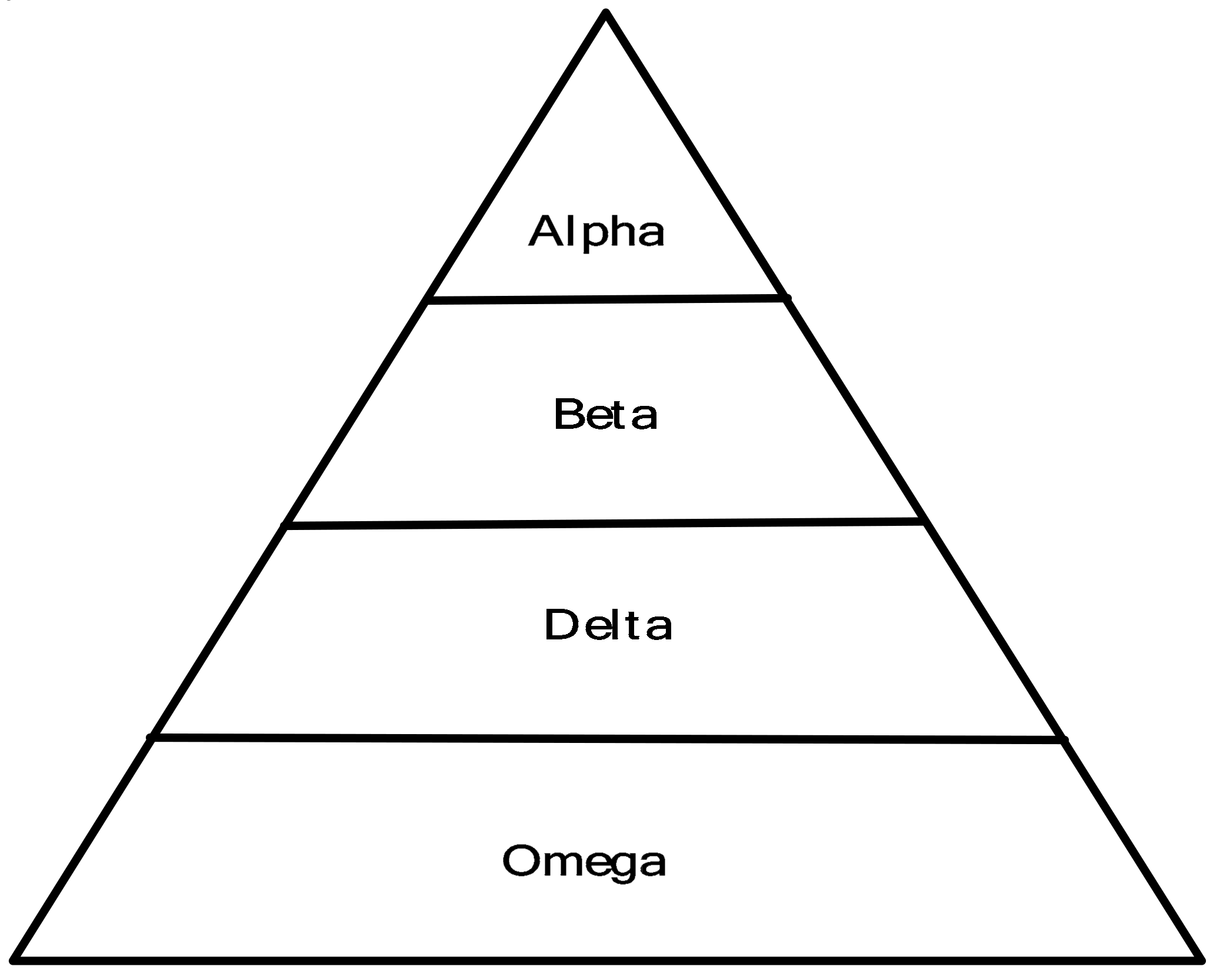
3.1. Grey Wolf Optimizer

GWO is a robust swarm-based optimizer inspired by the social hierarchy of grey wolves [27]. The pack of grey wolves has a special social hierarchy where the leadership in the pack can be divided into four levels; alpha, beta, omega and delta. Alpha wolf (α) is the first level in the social hierarchy hence it is the leader that guides the pack and the other wolves follow its orders. Beta wolf (β) is being in the second level of leadership that helps the alpha wolf directly for the activities of the pack. Delta (δ) wolves come in the third level of hierarchy where, they follow α and β wolves. The rest of wolves are the omegas (ω) that always have to submit to all the other dominant wolves. Figure 2 illustrates the social hierarchy ranking of wolves in GWO. In the mathematical model of GWO, the fittest solution is considered as the alpha (α), where, the second and third best solutions are called beta (β) and delta (δ), respectively. Finally, omega (ω) are considered the rest of the candidate solutions. However, the GWO based on three steps:
  • Encircling prey.
  • Hunting the prey.
  • Attacking the prey.

3.1.1. Encircling Prey

The grey wolves encircle the prey in hunting process that can be mathematically modeled as:
D = | C × X p ( i , j ) ( t ) X ( i , j ) ( t ) |
X ( i , j ) ( t + 1 ) = X p ( i , j ) ( t ) A × D
where, t is the current iteration, X p is the prey position vector, and X indicates the position vector of a grey wolf. A and C are coefficient vectors that can be calculated as:
A = 2 a × r 1 a
C = 2 × r 2
where, a is a value can be decreased linearly from 2 to 0 with iterations. r 1 and r 2 are random numbers in range [0, 1].

3.1.2. Hunting the Prey

In hunting process, the pack is affected by α , β and δ. Hence, the first three best solutions are saved as best agents ( α , β, δ) and the other search agents are updated their positions according to the best agents as:
D = | C × X p ( i , j ) ( t ) X ( i , j ) ( t ) |
D α = | C 1 × X α ( i , j ) X ( i , j ) |
D β = | C 2 × X β ( i , j ) X ( i , j ) |
D δ = | C 3 × X δ ( i , j ) X ( i , j ) |
X 1 ( i , j ) = X α ( i , j ) A 1 × ( D α )
X 2 ( i , j ) = X β ( i , j ) A 2 × ( D β )
X 3 ( i , j ) = X β ( i , j ) A 3 × ( D δ )
X ( i , j ) ( t + 1 ) = X 1 ( i , j ) + X 2 ( i , j ) + X 3 ( i , j ) 3
where, i is number of populations (vectors) and j is number of variables (individuals). A 1 , A 2 and A 3 are random vectors. The step size of the ω wolves is expressed in Equations (25)–(27), respectively. The final location of the ω wolves is formulated in Equations (28)–(31).

3.1.3. Attacking the Prey

The last stage in hunting is attacking the prey when the prey stopped. This can be achieved mathematically by reducing the value of a gradually from 2 to 0, consequently, A is varied randomly in range [−1, 1].

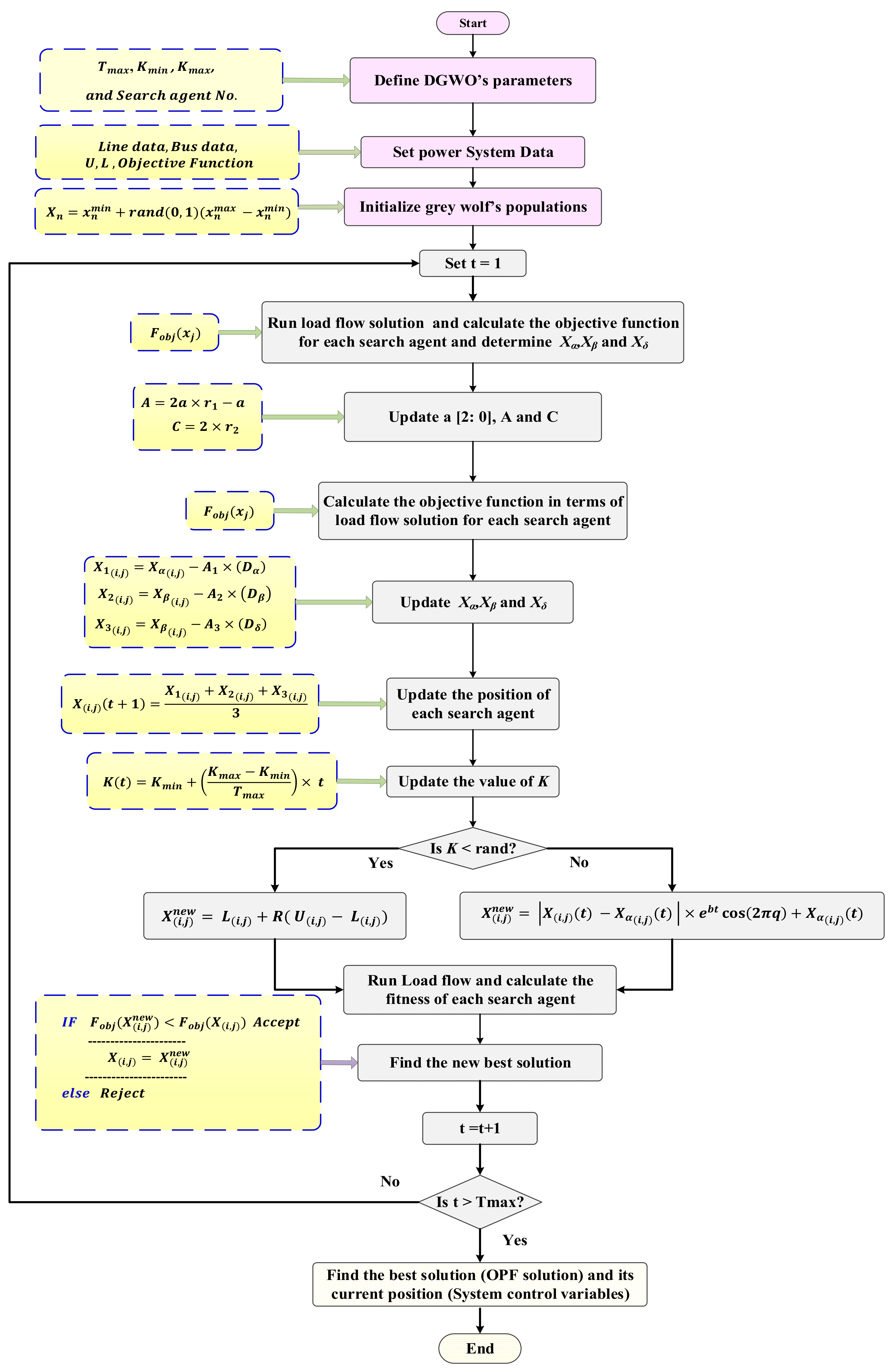
3.2. Developed Grey Wolf Optimizer

DGWO technique is presented as a new version for the conventional GWO. In this technique, the exploration and exploitation processes of GWO is enhanced. The exploration process is enhanced by integration a random mutation to find new searching regions to avoid the local minimum problem. The random mutation is applied as follows:
X ( i , j ) n e w = L ( i , j ) + R ( U ( i , j ) L ( i , j ) )
where, R is a random number over [0, 1]. X ( i , j ) n e w is a new generated vector. L and U are the lower and upper limits of control variables, respectively. In the exploitation of DGWO, the search process is focusing on the promising area by updating the search agents around the best solution ( X α ( i , j ) ) in logarithmic spiral function as:
X ( i , j ) n e w = | X ( i , j ) ( t ) X α ( i , j ) ( t ) | × e b t cos ( 2 π q ) + X α ( i , j ) ( t )
where:
  • X α ( i , j ) : the best position (alpha wolf position).
  • b: is a constant value for defining the logarithmic spiral shape.
  • q : is a random number [−1, 1].
For balancing the exploration during the initial searching process and exploitation in the final stages of the search process, an adaptive operator is used which changed dynamically as:
K ( t ) = K m i n + K m a x K m i n T m a x × t
The procedures of DGWO algorithm for solving the OPF problem can be summarized as follows:
(1)
Initialize maximum number of iterations ( T m a x ) and search agents (N).
(2)
Read the input system data.
(3)
Initialize grey wolf population X as:
X n = x n m i n + r a n d ( 0 , 1 ) ( x n m a x x n m i n )
where, n = 1 , 2 , 3 , j , x n m i n and x n m a x are the minimum and maximum limits of control variables which are predefined values. rand is a random number in range [0, 1].
(4)
Calculate the objective function for all grey wolf population using Newton Raphson load flow method.
(5)
Determine X α ( i , j ) , X β ( i , j ) , X δ ( i , j ) (first, second, and third best search agent).
(6)
Update the location of each search agent according Equations (24)–(31) and calculate the objective function using Newton Raphson load flow for the updated agents.
(7)
Update the values of a [2:0], A and C according Equations (22) and (23).
(8)
Update the adaptive operator, K according to Equation (34)
(9)
IF K < rand, update the position of search agent based on random mutation according to Equation (32)
ELSE IF K > rand, update the position of search agent locally in spiral path using Equation (33)
END
IF Fitness ( X ( i , j ) n e w ) < Fitness ( X ( i , j ) )
X ( i , j ) = X ( i , j ) n e w
ELSE, END
where, Fitness ( X ( i , j ) ) is the objective function of the position vector n while Fitness ( X ( i , j ) n e w ) is the objective function of the updated position vector j.
(10)
Repeat steps from (4) to (9) until the iteration number equals to its maximum value.
(11)
Find the best vector ( X α ( i , j ) ) which include the system control variables and its related fitness function.
However, the OPF solution process using the DGWO is shown in Figure 3.

4. Simulation Results

The DGWO is validated using the IEEE 30-bus test system. More details about this system can be found in [31]. The developed code has been written using MATLAB 2015 and the simulation run on a PC equipped with a core i5 processor, 2.50 GHz and 4 GB RAM. The upper and lower operating ranges and coefficients of generators are given in Table 1. The upper and lower limits of the load bus voltage are 1.05 p.u. and 0.95 p.u., respectively. The upper and lower limits of VAR compensation units are 0.00 p.u. and 0.05 p.u., respectively. The working voltage ranges of PV buses is [0.95, 1.1] p.u while the allowable range of transformer taps is [0.9, 1.1].The limits of transmission line power flows are given in [24]. The parameters of DGWO technique are selected as; number of populations = 50, maximum iteration = 100, b = 1, K m i n = 0.00001 and K m a x = 0.1. In this study, 100 runs have been performed for all the test cases to calculate the best cost, the worst cost and the average cost.

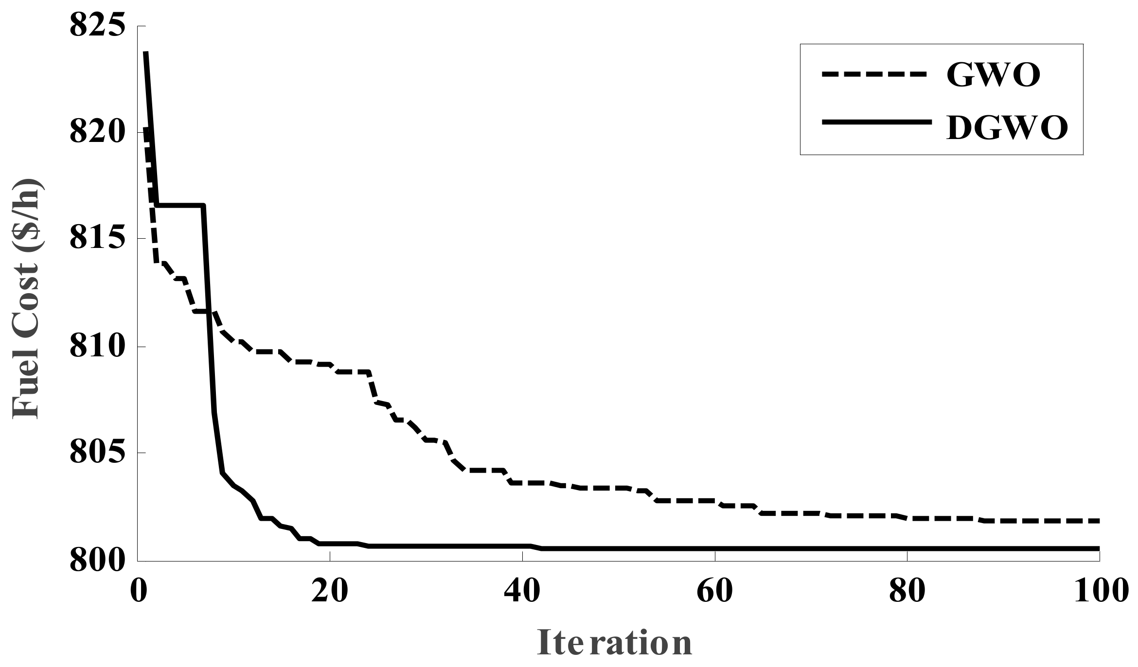
4.1. Case1: OPF Solution without Considering the Valve Point Effects

In this case, the quadratic fuel cost effect is taken as an objective function to be minimized as given in Equation (6). The generator data for this case are listed in Table 1. The optimal control variables for this case obtained by GWO and DGWO techniques are listed in 4th and 5th columns of Table 2, respectively. The obtained fuel cost using GWO and DGWO are 801.259 $/h and 800.433 $/h, respectively. Table 3 gives the fuel costs obtained by GWO, DGWO and other optimization techniques. From Table 3, it can be observed that the obtained results using DGWO are better than those obtained by the others reported optimization techniques in terms of the best, the worst and the average fuel costs. The convergence characteristics of GWO and DGWO for this case are shown in Figure 4. It is clear that DGWO has stable and rapid convergence characteristic.

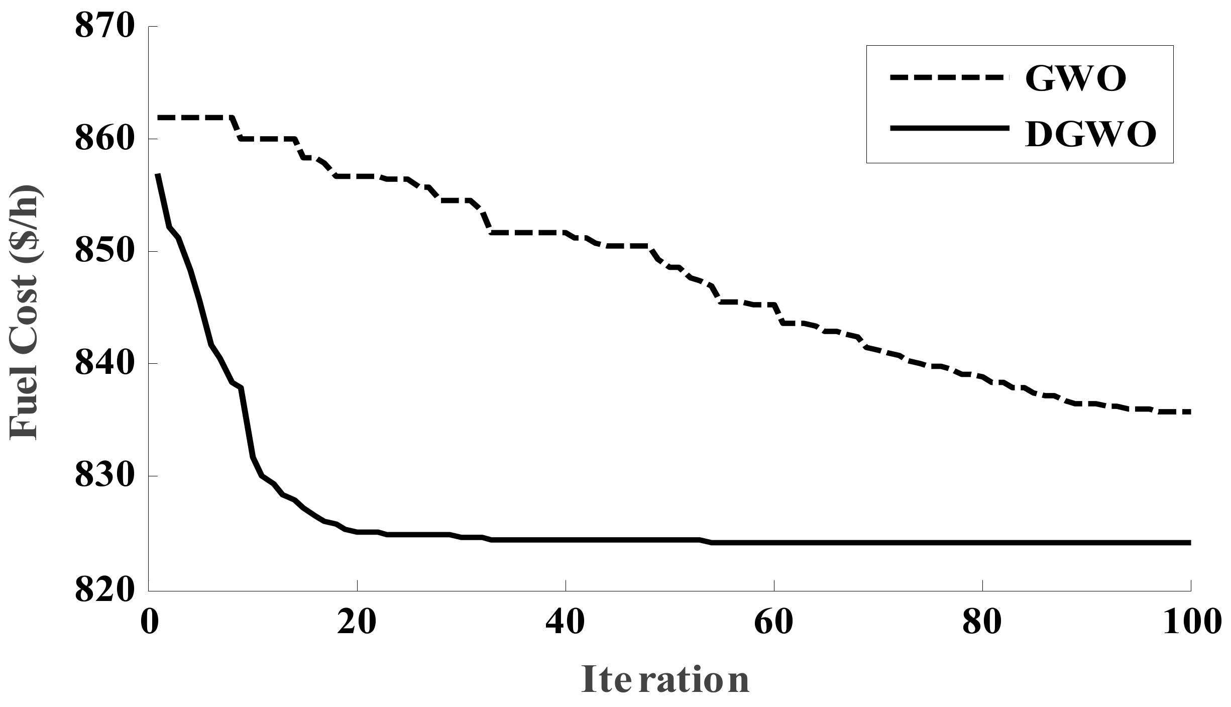
4.2. Case 2: OPF Solution Considering the Valve Point Effects

In this case, the OPF problem is solved considering the valve point effect as given in Equation (7). The optimal control variables obtained by the DGWO are given in 6th and 7th columns of Table 2, respectively. The minimum fuel costs obtained by GWO and DGWO are 830.028 $/h and 824.132 $/h, respectively. Table 4 gives the fuel costs obtained by DGWO, GWO, and other techniques under the same conditions (control variable boundaries, dependent variables limits and system constraints).
From Table 4, it can be observed that the obtained results from DGWO are better than those obtained by GWO and the other techniques. Figure 5 shows the convergence characteristics of the minimum fuel cost of the GWO and DGWO. From this figures, it can be observed that the DGWO is converged faster than GWO.
Table 2 gives the active power losses, voltage stability index and summation of voltage deviations. From this table, it can be observed that some values are increased for DGWO compared with GWO, this due to these values are not considered as objective functions. As it is well known that the optimization of single objective function probably not lead to enhance the other functions.

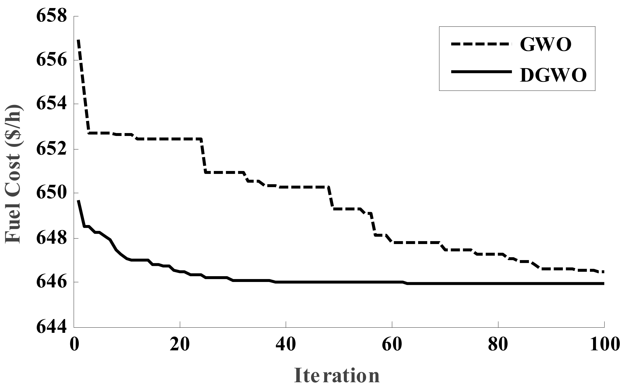
4.3. Case 3: OPF Solution Considering Piecewise Quadratic Fuel Cost Function

In this case, piecewise fuel cost function is taken as an objective function as given in Equation (8). In this case, two generation units at buses 1 and 2 are represented by piecewise quadratic cost functions [16]. The generated active power and the generation unit coefficients for this case are given in Table 5. The optimal control variables obtained by GWO and DGWO are listed in 8th and 9th columns of Table 2, respectively. The minimum piecewise fuel costs obtained by GWO and DGWO are 646.426 $/h and 645.913 $/h, respectively. The piecewise fuel costs obtained by DGWO, GWO, and other techniques given in Table 6. From Table 6, it can be observed that the obtained results from DGWO are better than those obtained by GWO and the other techniques in terms of the best, the worst and the average piecewise fuel costs. Figure 6 shows the convergence characteristics of the minimum fuel cost of the GWO and DGWO for this case. It is clear that DGWO has fast and stable convergence characteristic compared with GWO.

5. Conclusions

In this paper, DGWO has been proposed to efficiently solve the OPF problem and avoid the stagnation problems of the traditional GWO. This technique is based on modifying the grey wolf optimizer by employing a random mutation for enhancing its exploration process. This modification provides a flexibility to search in new areas. Moreover, the new generated populations are updated around the best solution in a spiral path to enhance the exploitation process and focus on the most promising areas. In the proposed technique, two equations should be added to the traditional GWO, the first equation is related to the random mutation and the second one for the spiral path updating process. The results obtained by the proposed algorithm have been compared with those obtained by the conventional GWO and other well-known optimization techniques. From the results obtained, it can be concluded that:
-
The proposed technique has successfully performed to find the optimal settings of the control variables of test system.
-
Different objective functions (quadratic fuel cost minimization, piecewise quadratic cost minimization, and quadratic fuel cost minimization considering the valve point effect) have been achieved using the proposed algorithm.
-
The superiority of DGWO compared with the conventional GWO and other well-known optimization techniques has been proved.
-
DGWO has a fast and stable convergence characteristic compared with the conventional GWO.
In the future work, the proposed algorithm will be applied in other planning and expansion studies in power systems with thermal and renewable generation units considering the uncertainties of load.

Author Contributions

M.A., S.K. and M.E. proposed the idea, obtained the results, and wrote the paper. J.Y. and F.J. contributed by drafting and critical revisions. All authors together organized and refined the manuscript in the present form.

Funding

This work was supported in part by the Project Supported by the National Key Research and Development Program of China under grant 2017YFB0902200, the Basic and Frontier Research Project of Chongqing under grant cstc2017jcyjBX0056, the Academician Lead Science and Technology Innovation Guide Project of Chongqing under grant cstc2017jcyj-yszxX0011 and the Fundamental Research Funds for the Central Universities 2018CDQYDQ0006.

Conflicts of Interest

The authors declare no conflict of interest.

Nomenclature

ABCArtificial bee colony algorithm
BSABacktracking search algorithm
DGWODeveloped grey wolf optimizer
GAGenetic algorithm
GWOGrey wolf optimizer
LPLinear programming
MSAMoth swarm algorithm
OPFOptimal power flow
QPQuadratic programming
TS Tabu search
MFOMoth-flame algorithm
ITSImproved Tabu Search
A 1 ,   A 2 ,   A 3 Random vectors
xThe state variables vector
L , U The lower and upper boundary of control variables
QGThe reactive power output of generators
tThe current iteration
T max The maximum number of iterations
P D i , Q D i The active and reactive load demand at bus i
δ i j Phase difference of voltages
VLThe voltage of load bus
VGThe voltage of generation bus
NPQNumber of load buses
di, eiThe fuel cost coefficients of the ith generator unit with valve-point effects
NTLNumber of transmission lines
RRandom number
rand Random value
G Transmission line conductance
B Transmission line susceptance
X p The prey position vector
kAdaptive operator
bConstant value
K G , K Q , K V , K S , K S Penalty factors
X α , X β , X δ First, second, and third best search agents
max, minSuperscript refers to maximum and minimum values
BBOBiogeography-based optimization
DEDifferential evolution
EPEvolutionary programming
GSAGravitational search algorithm
MDEModified differentia evolution
NLPNonlinear programming
PSOParticle swarm optimization
SFLAShuffle frog leaping algorithm
SOSSymbiotic organisms search
TLBOTeaching–learning-based optimization
IPInterior point
FThe objective function
gi, hjThe equality and inequality constraints
uThe control variables vector
m, pNumber of equality and inequality constraints
QCThe injected reactive power of shunt compensator
PG1The generated power of slack bus
PGThe output active power of generator
SLThe apparent power flow in transmission line
TTap setting of transformer
NGNumber of generators
NCNumber of shunt compensator
NT Number of transformers
NPVNumber of generators PV buses
ai, bi, ciThe cost coefficients of ith generator.
NPVNumber of generation buses
ICurrent
VMagnitude of node voltage
R, X, ZResistance, reactance, impedance
P, Q, SActive, reactive, apparent powers
X The location of the present solution
q A random number
X n e w New generated vector
α , β , δ , ω Alpha, beta, delta, omega fittest solutions
C , C 1 , C 2 , C 3 Random vectors

References

  1. Lee, K.; Park, Y.; Ortiz, J. A united approach to optimal real and reactive power dispatch. IEEE Trans. Power Appar. Syst. 1985, PER-5, 1147–1153. [Google Scholar] [CrossRef]
  2. Zhu, J. Optimization of Power System Operation; John Wiley & Sons: Hoboken, NJ, USA, 2015; Volume 47. [Google Scholar]
  3. Dommel, H.W.; Tinney, W.F. Optimal power flow solutions. IEEE Trans. Power Appar. Syst. 1968, PAS-87, 1866–1876. [Google Scholar] [CrossRef]
  4. Mota-Palomino, R.; Quintana, V. Sparse reactive power scheduling by a penalty function-linear programming technique. IEEE Trans. Power Syst. 1986, 1, 31–39. [Google Scholar] [CrossRef]
  5. Burchett, R.; Happ, H.; Vierath, D. Quadratically convergent optimal power flow. IEEE Trans. Power Appar. Syst. 1984, PAS-103, 3267–3275. [Google Scholar] [CrossRef]
  6. Santos, A.J.; da Costa, G. Optimal-power-flow solution by Newton’s method applied to an augmented Lagrangian function. IEE Proc. Gener. Transm. Distrib. 1995, 142, 33–36. [Google Scholar] [CrossRef]
  7. Yan, X.; Quintana, V.H. Improving an interior-point-based OPF by dynamic adjustments of step sizes and tolerances. IEEE Trans. Power Syst. 1999, 14, 709–717. [Google Scholar]
  8. Chung, T.; Li, Y. A hybrid GA approach for OPF with consideration of FACTS devices. IEEE Power Eng. Rev. 2000, 20, 54–57. [Google Scholar] [CrossRef]
  9. Paranjothi, S.; Anburaja, K. Optimal power flow using refined genetic algorithm. Electr. Power Compon. Syst. 2002, 30, 1055–1063. [Google Scholar] [CrossRef]
  10. Ebeed, M.; Kamel, S.; Youssef, H. Optimal setting of STATCOM based on voltage stability improvement and power loss minimization using Moth-Flame algorithm. In Proceedings of the 2016 Eighteenth International Middle East Power Systems Conference (MEPCON), Cairo, Egypt, 27–29 December 2016; pp. 815–820. [Google Scholar]
  11. Varadarajan, M.; Swarup, K.S. Solving multi-objective optimal power flow using differential evolution. IET Gener. Transm. Distrib. 2008, 2, 720–730. [Google Scholar] [CrossRef]
  12. Abou El Ela, A.A.; Abido, M.; Spea, S. Optimal power flow using differential evolution algorithm. Electr. Power Syst. Res. 2010, 80, 878–885. [Google Scholar] [CrossRef]
  13. Abido, M. Optimal power flow using particle swarm optimization. Int. J. Electr. Power Energy Syst. 2002, 24, 563–571. [Google Scholar] [CrossRef]
  14. Mohamed, A.-A.A.; Mohamed, Y.S.; El-Gaafary, A.A.; Hemeida, A.M. Optimal power flow using moth swarm algorithm. Electr. Power Syst. Res. 2017, 142, 190–206. [Google Scholar] [CrossRef]
  15. Ongsakul, W.; Tantimaporn, T. Optimal power flow by improved evolutionary programming. Electr. Power Compon. Syst. 2006, 34, 79–95. [Google Scholar] [CrossRef]
  16. Yuryevich, J.; Wong, K.P. Evolutionary programming based optimal power flow algorithm. IEEE Trans. Power Syst. 1999, 14, 1245–1250. [Google Scholar] [CrossRef]
  17. Adaryani, M.R.; Karami, A. Artificial bee colony algorithm for solving multi-objective optimal power flow problem. Int. J. Electr. Power Energy Syst. 2013, 53, 219–230. [Google Scholar] [CrossRef]
  18. Duman, S.; Güvenç, U.; Sönmez, Y.; Yörükeren, N. Optimal power flow using gravitational search algorithm. Energy Convers. Manag. 2012, 59, 86–95. [Google Scholar] [CrossRef]
  19. Bhattacharya, A.; Chattopadhyay, P. Application of biogeography-based optimisation to solve different optimal power flow problems. IET Gener. Transm. Distrib. 2011, 5, 70–80. [Google Scholar] [CrossRef]
  20. Niknam, T.; Narimani, M.R.; Azizipanah-Abarghooee, R. A new hybrid algorithm for optimal power flow considering prohibited zones and valve point effect. Energy Convers. Manag. 2012, 58, 197–206. [Google Scholar] [CrossRef]
  21. Shaheen, A.M.; El-Sehiemy, R.A.; Farrag, S.M. Solving multi-objective optimal power flow problem via forced initialised differential evolution algorithm. IET Gener. Transm. Distrib. 2016, 10, 1634–1647. [Google Scholar] [CrossRef]
  22. Abido, M. Optimal power flow using tabu search algorithm. Electr. Power Compon. Syst. 2002, 30, 469–483. [Google Scholar] [CrossRef]
  23. Sayah, S.; Zehar, K. Modified differential evolution algorithm for optimal power flow with non-smooth cost functions. Energy Convers. Manag. 2008, 49, 3036–3042. [Google Scholar] [CrossRef]
  24. Duman, S. Symbiotic organisms search algorithm for optimal power flow problem based on valve-point effect and prohibited zones. Neural Comput. Appl. 2017, 28, 3571–3585. [Google Scholar] [CrossRef]
  25. Kılıç, U. Backtracking search algorithm-based optimal power flow with valve point effect and prohibited zones. Electr. Eng. 2015, 97, 101–110. [Google Scholar] [CrossRef]
  26. Ghasemi, M.; Ghavidel, S.; Gitizadeh, M.; Akbari, E. An improved teaching–learning-based optimization algorithm using Lévy mutation strategy for non-smooth optimal power flow. Int. J. Electr. Power Energy Syst. 2015, 65, 375–384. [Google Scholar] [CrossRef]
  27. Mohammadi, A.; Mehrtash, M.; Kargarian, A. Diagonal quadratic approximation for decentralized collaborative TSO+ DSO optimal power flow. IEEE Trans. Smart Grid 2018. [Google Scholar] [CrossRef]
  28. Naderi, E.; Azizivahed, A.; Narimani, H.; Fathi, M.; Narimani, M.R. A comprehensive study of practical economic dispatch problems by a new hybrid evolutionary algorithm. Appl. Soft Comput. 2017, 61, 1186–1206. [Google Scholar] [CrossRef]
  29. Mirjalili, S.; Mirjalili, S.M.; Lewis, A. Grey wolf optimizer. Adv. Eng. Softw. 2014, 69, 46–61. [Google Scholar] [CrossRef]
  30. Azizivahed, A.; Narimani, H.; Fathi, M.; Naderi, E.; Safarpour, H.R.; Narimani, M.R. Multi-objective dynamic distribution feeder reconfiguration in automated distribution systems. Energy 2018, 147, 896–914. [Google Scholar] [CrossRef]
  31. IEEE 30-Bus Test System Data. Available online: https://www.ee.washington.edu/research/pstca/pf57/pg_tca30bus.hm (accessed on 26 June 2018).
Figure 1. Cost function with and without valve point effect.
Energies 11 01692 g001
Figure 2. Social hierarchy of wolves in GWO.
Energies 11 01692 g002
Figure 3. The solution process of OPF problem using DGWO.
Energies 11 01692 g003
Figure 4. Convergence characteristics of fuel cost (Case 1).
Energies 11 01692 g004
Figure 5. Convergence characteristics of fuel cost (Case 2).
Energies 11 01692 g005
Figure 6. Convergence characteristics of fuel cost (Case 3).
Energies 11 01692 g006
Table 1. Generator data coefficients.
Bus No. P G m a x   ( M W ) P G m i n   ( M W ) Q G m i n   ( M V a r ) Cost CoefficientsProhibited Zones
abc
125050−2002.00.00375(55–66), (80–120)
28020−2001.750.0175(21–24), (45–55)
55015−1501.00.0625(30–36)
83510−1503.250.00834(25–30)
113010−1003.000.025(25–28)
134012−1503.000.025(24–30)
Table 2. Optimal control variables for different cases obtained by GWO and DGWO.
VariablesLimitCase 1Case 2Case 3
Min.Max.GWODGWOGWODGWOGWODGWO
P1 (MW)50250171.094176.949212.633219.801140.00140.00
P2 (MW)208048.61548.51925.68428.35854.99255.000
P5 (MW)155021.12321.32617.61215.04734.93024.105
P8 (MW)103522.06821.57114.18510.00025.00835.000
P11 (MW)103015.47912.02610.65110.00016.93418.239
P13 (MW)124013.66512.00113.75112.00018.22317.664
V1 (p.u)0.951.11.0801.0831.0871.0901.0771.073
V2 (p.u)0.951.11.0621.0631.0621.0651.0641.060
V5 (p.u)0.951.11.0301.0311.0231.0321.0351.032
V8 (p.u)0.951.11.0361.0351.0351.0351.0441.040
V11 (p.u)0.951.11.0801.0601.0511.0991.0621.049
V13 (p.u)0.951.11.0541.0501.0601.0371.0361.060
T110.901.10.9820.9771.01280.9481.0230.994
T120.901.11.0261.0130.9081.0251.0080.978
T150.901.10.9890.9340.9860.9701.0190.971
T360.901.10.9810.9750.9760.9810.9590.975
Q10 (MVar)0.005.002.1441.6953.1703.2770.9861.251
Q12 (MVar)0.005.002.9293.3942.1432.3673.9963.157
Q15 (MVar)0.005.001.4004.7771.9591.2282.9782.433
Q17 (MVar)0.005.003.5264.1531.1264.6602.1484.831
Q20 (MVar)0.005.002.9543.7382.3693.5854.1394.462
Q21 (MVar)0.005.003.5884.9412.0163.6032.8784.653
Q23 (MVar)0.005.002.9743.5671.5323.5603.6033.043
Q24 (MVar)0.005.003.6884.9961.6754.6031.3774.467
Q29 (MVar)0.005.003.2592.2002.3783.2323.6282.439
PLoss(MW)NANA8.64288.992111.115111.8056.68606.6079
VD (p.u)NANA0.72850.87840.70550.85890.61700.8825
Lmax (p.u)NANA0.12990.12790.13280.12810.13070.1280
Fuelcost ($/h)NANA801.259800.433830.028824.132646.426645.913
Computational time (s)NANA53.637.841.7041.552.447.2
PLoss: Power losses, Lmax: Voltage stability index, VD: Summation voltage deviations.
Table 3. Simulation results of Case 1.
AlgorithmBest CostAverage CostWorst Cost
DGWO800.433800.4674800.4989
GWO801.259802.663804.898
MSA [14]800.5099NANA
SOS [24]801.5733801.7251801.8821
ABC [17]800.6600800.8715801.8674
TS [22]802.290NANA
MDE [23]802.376802.382802.404
IEP [15]802.465802.521802.581
TS [15]802.502802.632802.746
EP [16]802.62803.51805.61
TS/SA [15]802.788803.032803.291
EP [15]802.907803.232803.474
ITS [15]804.556805.812806.856
GA [9]805.937NANA
Table 4. Comparison of the simulation results of Case 2.
AlgorithmBest CostAverage CostWorst Cost
DGWO824.132824.295824.663
GWO830.028844.639852.388
SOS [24]825.2985825.4039825.5275
BSA [25]825.23827.69830.15
SFLA-SA [20]825.6921NANA
SFLA [20]825.9906NANA
PSO [20]826.5897NANA
SA [20]827.8262NANA
Table 5. Cost coefficients of generators (Case 3).
Bus No.Output Power Limit (MW)Cost Coefficients
Min.Max.abc
15014055.00.700.0050
14020082.51.050.0075
2205540.00.300.0100
558080.00.600.0200
Table 6. Comparison of the simulation results of Case 3.
AlgorithmBest CostAverage CostWorst Cost
DGWO645.9132645.993646.095
GWO646.426647.432648.681
GSA [18]646.8480646.8962646.9381
Lévy LTLBO [26]647.4315647.4725647.8638
PSO [13]647.69647.73647.87
BBO [19]647.7437647.7645647.7928
TLBO [26]647.8125647.8335647.8415
MDE [23]647.846648.356650.664
ABC [17]649.0855654.0784659.7708
EP [16]650.206654.501657.120
TS [15]651.246654.087658.911
TS/SA [15]654.378658.234662.616
ITS [15]654.874664.473675.035

