Convex Programming and Bootstrap Sensitivity for Optimized Electricity Bill in Healthcare Buildings under a Time-Of-Use Pricing Scheme

Abstract

Efficient energy management is strongly dependent on determining the adequate power contracts among the ones offered by different electricity suppliers. This topic takes special relevance in healthcare buildings, where noticeable amounts of energy are required to generate an adequate health environment for patients and staff. In this paper, a convex optimization method is scrutinized to give a straightforward analysis of the optimal power levels to be contracted while minimizing the electricity bill cost in a time-of-use pricing scheme. In addition, a sensitivity analysis is carried out on the constraints in the optimization problems, which are analyzed in terms of both their empirical distribution and their bootstrap-estimated statistical distributions to create a simple-to-use tool for this purpose, the so-called mosaic-distribution. The evaluation of the proposed method was carried out with five-year consumption data on two different kinds of healthcare buildings, a large one given by Hospital Universitario de Fuenlabrada, and a primary care center, Centro de Especialidades el Arroyo, both located at Fuenlabrada (Madrid, Spain). The analysis of the resulting optimization shows that the annual savings achieved vary moderately, ranging from −0.22 % to +27.39%, depending on the analyzed year profile and the healthcare building type. The analysis introducing mosaic-distribution to represent the sensitivity score also provides operative information to evaluate the convenience of implementing energy saving measures. All this information is useful for managers to determine the appropriate power levels for next year contract renewal and to consider whether to implement demand response mechanisms in healthcare buildings.

1. Introduction

Conventionally, demand side management (DSM) is defined as the planning, implementation, and monitoring of distribution network utility activities designed to influence the customer use of electricity in a way that will produce some desired changes in the time pattern and load magnitude [1,2]. Even tough DSM is still an active research topic with significant practical implications in the electrical industry, DSM scope has evolved rapidly in the last decade, mainly due to the improved communication and control capabilities offered by modern information and communications technologies (ICTs). In particular, the load management concept has evolved into the so-called Demand Response (DR) [3]. DR schemes depend on the entities involved (i.e., electricity market, utility, and customers) and the objective of the DR request (i.e., Price-Based DRs and Physical DRs). Pricing schemes can range from simple (e.g., single, flat, or block rates) to complex rates, such as seasonal, time-of-use (TOU), or real-time pricing (RTP) rates. Nevertheless, TOU pricing is the most worldwide employed scheme for electrical energy billing [4,5,6]. On the other hand, physical-DR request may include load shifting, turning-off non-essential loads, peak shaving, or turning-on allowable on-site generators [7], and more recently the so-called battery energy storage systems (BESS) [8]. In this context, a very special kind of industrial consumers which need to adopt DR programs are healthcare buildings, as they usually are large and complex buildings that are continuously operating, consuming energy on large scale, and playing a vital role in health services [9,10,11]. Energy needs of large hospitals can be comparable to a small city and they manage expensive electricity bills. This considerable energy consumption and its subsequent billing require an effective load management to obtain savings without affecting the quality of service in the patient healthcare [12].

Before adopting a DR program, facility managers need to analyze the energy performance to quantify the cost associated with energy consumption and to quantify the impact of implementing those DRs actions that require investment, finance viability and payback time [13,14]. In this regard, the aim of this paper is to support healthcare building managers in adopting a Price-Based DR program, specifically in a TOU pricing scheme. For this purpose, we formulate the DR problem subject to TOU pricing constraints based on convex optimization that finds the contracted power level that minimizes the cost of electricity bill and satisfies the TOU pricing. Convex optimization is a widely used tool for this purpose, and it refers to the minimization of a convex objective function subject to convex constraints [15]. Not only can convex optimization provide with a direct solution of the most convenient power level by block rate to be contracted by a healthcare building in terms of the its power demand, but it can also provide the sensitivity of the problem to the involved constraints, although it could be highly informative from a managerial point of view.

To our best knowledge, the literature review provides limited information about the optimization of the electricity bill with data from this special type of customer. Most of the existing research related to TOU rates is concerned about utilities and industrial customers, and these approaches exhibit different mathematical methods. Among others, several complex methods were considered in [16,17,18] as optimization approaches. In [16], the authors studied mathematical models for the consumer and the utility companies to optimize the cost to the parties individually and in combination. In [17], an approach was proposed for TOU design based in quadratically constrained quadratic programming and stochastic optimization techniques from the utility point of view. Furthermore, in [18] a game-theoretic approach is considered for optimal TOU electricity pricing. Other works (e.g., [19,20]) have focused on evaluating electricity rates though characterization and forecasting of energy consumption to advise companies for the contract renewal. All these studies have different approaches from ours and they have paid little attention to the sensitivity analysis.

We evaluated our approach on two different kinds of healthcare buildings: (1) a recently created hospital with modern facilities and general design, which virtually represents a small city itself, i.e., Hospital Universitario de Fuenlabrada (HUF); and (2) a primary healthcare center referred to it, namely Centro de Especialidades el Arroyo (CEA), with lower power consumption. Both are located in the city of Fuenlabrada (Spain) and can provide us with a contrasted and differential analysis on their energy consumption on the basis of a shared geographical and demographical context.

The main contributions of this paper can be summarized as follows. First, we propose a novel yet simple methodology based on convex programming that allows us to determine the optimal power levels to be contracted with the electricity company into a TOU-rate scheme. Second, we model the sensitivity of the annual cost of energy by block and period, and use non-parametric resampling techniques (specifically, bootstrap resampling [21]) to generate an easy-to-handle tool for analyzing the sensitivity of the cost in terms of months and consumption blocks, in a unified statistical form. This proposal allowed us to identify at a glance where the demanded power exceeded the contracted power and its impact from a statistical point of view. This sensitivity analysis using mosaic distributions can straightforwardly drive managers towards the specific TOU block where DR programs need to be prioritized and implemented, hence supporting an improved energy management in healthcare buildings; however, the entire approach could also be useful in other scenarios.

The rest of this paper is organized as follows. In Section 2, we formulate the DR problem subject to TOU pricing scheme, and we detail the methodology used for sensitivity analysis. In Section 3, we describe the datasets, corresponding to the two aforementioned healthcare buildings, as well as the blocks of the TOU rates considered in this work. In Section 4, we present the experimental results in pricing optimization and sensitivity analysis for both scenarios (large and small scale healthcare buildings). Finally, Section 5 summarizes the discussion and main conclusions of this work.

2. Demand Response Optimization: Sensitivity Analysis and Mosaic Distribution

In this section, we formulate the DR problem subject to TOU pricing constraints. More specifically, we formulate a constrained optimization problem that, using as inputs the power demand and the pricing schemes, finds the contracted power level that minimizes the cost and satisfies the TOU pricing constraints imposed by the operator. This optimization will be the key not only to finding the optimal contracted powers, but also to analyzing the sensitivity of the solutions with respect to changes in the power demand. To that end, the first part of the section focuses on the problem formulation and discusses how this problem could be solved using convex programming tools [22]. The second part addresses the sensitivity analysis by discussing the empirical distribution of the Lagrange multipliers (LM) associated with the optimization, and the usefulness of the bootstrap re-sampling techniques [21] to yield a unified view of the relevance of the constraints through different blocks and month periods.

Regarding the problem formulation, we start by introducing the main notational conventions and, then, identify the state variables (which serve as inputs to our problem), the optimization variables (which serve as outputs), the constraints relating the different variables, and the cost to minimize.

• Power consumption. We focus on optimizing the power consumption during one year (12 months) and consider that the time is divided into regularly sampled 15-min periods. Variable N is used to denote the total number of periods in a year (i.e., $N=365\times 24\times 4$) and variable n is used to index those periods of 15 min each). Similarly, we use $M=12$ to denote the total number of months in a year and the variable m to index the corresponding month. With this notation in place, we can define the column vector $\mathbf{d}\in {\mathbb{R}}^N$ as the one-year load consumption (in kWh). Moreover, suppose that at period n the contracted power is not enough to meet the current demand, thus additional power from the supplier are needed. Then, we use $x_n$ to denote the excess power at period n (in kW) and collect all those values in vector $\mathbf{x}\in {\mathbb{R}}^N$. Defining $N_m$ as the number of 15-min periods in month m, we also define the monthly counterparts of the previous vectors as ${\mathbf{d}}_m\in {\mathbb{R}}^{N_m}$ and ${\mathbf{x}}_m\in {\mathbb{R}}^{N_m}$ and write ${\mathbf{d}}^{\top }=[{\mathbf{d}}_1^{\top },\dots ,{\mathbf{d}}_M^{\top }]$ and ${\mathbf{x}}^{\top }=[{\mathbf{x}}_1^{\top },\dots ,{\mathbf{x}}_M^{\top }]$.
• Pricing mechanisms. The operator considers $T=6$ different tariff periods, which are indexed by variable t. The unitary cost of the power during the tariff period t is denoted as $c_t$, and all those prices are collected in vector $\mathbf{c}\in {\mathbb{R}}^T$. At the beginning of each year, the customer must decide the amount of power that is contracted for each of the tariff periods. To that end, we use $p_t$ to denote the contracted power at tariff period t and collect all those variables in the column vector $\mathbf{p}\in {\mathbb{R}}^T$. Moreover, to penalize the amount of excess power that the customer needs to buy every month, the supplying company establishes a cost coefficient $k_t$ for each tariff t, which are collected in the column vector. Finally, to account for the TOU pricing mechanism, we consider the binary variable $Q_{n,t}^m$, which is one if the time period n of the month m is charged with the tariff t and zero otherwise. Moreover, for each month m and tariff t, we can collect the corresponding binary variables in the vector ${\mathbf{q}}_t^m\in {\mathbb{R}}^{N_m}$. Those vectors are used to define the diagonal matrices $\mathrm{diag}\left({\mathbf{q}}_t^m\right)$ for all $(m,t)$ as well as the matrices ${\mathbf{Q}}^m=[{\mathbf{q}}_1^m,\dots ,{\mathbf{q}}_T^m]\in {\mathbb{R}}^{N_m\times T}$ for all m.

Using the state variables $\mathbf{p}$, $\mathbf{c}$ and $\mathbf{k}$ as inputs, and viewing the optimization variables $\mathbf{p}$ and $\mathbf{x}$ as outputs, our DR optimization problem subject to TOU constraints can be formulated as

$$\begin{array}{cc}\hfill J(\mathbf{c},\mathbf{k},\mathbf{d}):=\underset{\mathbf{p},\mathbf{x}}{\min }& \sum _{t=1}^T{c}_t{p}_t+\sum _{t=1}^T\sum _{m\in M}{k}_t{\Vert \mathrm{diag}\left({\mathbf{q}}_t^m\right){\mathbf{x}}_m\Vert }_2\hfill \end{array}$$

(1)

$$\begin{array}{cc}\hfill \mathrm{subject}\mathrm{to}:& \mathbf{p}\ge 0,{\mathbf{x}}_m\ge 0,\forall m=1,\dots ,M,\hfill \end{array}$$

(2)

$$\begin{array}{c}\hfill {\mathbf{Q}}^m\mathbf{p}+{\mathbf{x}}_m\ge {\mathbf{d}}_m,\forall m=1,\dots ,M,\end{array}$$

(3)

$$\begin{array}{c}\hfill p_t\le p_{t+1},\forall t=1,\dots ,T-1,\end{array}$$

(4)

$$\begin{array}{c}\hfill p_T\ge p_{min}.\end{array}$$

(5)

In the above optimization, the constraints in Equation (2) account for the fact that the power variables are non-negative; Equation (3) are balance constraints that guarantee that the power demand is always satisfied; and the constraints in Equations (4) and (5) are imposed by the power supplier as part of its TOU pricing mechanisms. Regarding the cost, we note that two terms are considered. The first one simply accounts for the cost of the power contracted at the beginning of the year for each of the T tariffs. The second one, which is a bit more involved, accounts for the excess of power that the customer must buy when the demand exceeds the contracted power. More specifically, this second term considers all month–tariff pairs and, for a given $(t,m)$ pair, finds the cost as the multiplication of the coefficient $k_t$ with the ${\ell }_2$ norm of the vector collecting the excesses during the $(t,m)$ pair, which can be conveniently obtain as $\mathrm{diag}\left({\mathbf{q}}_t^m\right){\mathbf{x}}_m$.

All the constraints in Equations (1)–(5) are linear; the cost to minimize is the sum of a linear term and ${\ell }_2$ norms; and the domains of the optimization variables are ${\mathbb{R}}^N$. As a result, the formulated problem is convex and can be efficiently solved, either upon developing tailored first/second order algorithms (recommended when computational complexity is an issue), or using a generic off-the-shelf solver such as CVX (if the dimensionality of the problem is not large) [22].

Note that, if $\mathbf{c}$, $\mathbf{k}$ and $\mathbf{d}$ are given, the formulated optimization yields the value of $\mathbf{p}$ that minimizes the cost paid by the customer. Unfortunately, while the prices $\mathbf{c}$ and $\mathbf{k}$ are known at the beginning of the year, the demand $\mathbf{d}$ is not. Different approaches arise to handle this issue. If the joint probability distribution of $\mathbf{d}$ is known, the optimization can be reformulated as a stochastic problem whose objective is to minimize, for example, an average or a worst-case cost. Alternatively, one can use as input the demand of the previous year and, then, analyze the sensitivity of the problem to variations of such a demand, which is is one of the goals of the ensuing section.

2.1. Sensitivity Analysis

Whereas it is easy to identify the time instants when the consumption has overpassed the power limits, it is not so immediate to provide with an operative view on which are the periods for each month when the consumption is statistically closer or over the limits. An intuitive and heuristic solution should be to represent the histograms of the consumption excesses per block and month period. Two improvements can be done to this simple approach. On the one hand, the use of the sensitivities provided by the convex optimization solver for the excess constrains is statistically more representative than that of the empirical values of the overshoots itself, because, for instance, the LM associated with the constraints are less affected by outliers or atypical samples. On the other hand, the statistical distribution of the sensitivities are often complex, probably a mix of a Bernoulli distribution with another continuous distribution (e.g., Bernoulli–Gaussian) due to the time instants per block and month when the consumption remains below the limit are associated with a null Lagrange multiplier. This can be arranged by the estimation of the average value, and improved by yielding the statistical distribution of that average value per period and month, which can be tackled efficiently using bootstrap resampling the available on the yearly consumption samples and on the optimization problem statement.

The sensitivity analysis in convex optimization [22,23] aims to quantify the impact on the solution of the constrains, either all of them, or some subset of special interest. If we denote by $v^{t,k}$ the LM associated with the constraints in Equation (3), those LM represent the sensitivity of the optimization cost with respect to the variation on the demand (and, hence, on power consumption excess), taking into account their distribution in periods and months, as required by the optimization primal functional. The empirical distribution functions for these Lagrange multipliers can be expressed as

$$\widehat{f_e}\left(v^{t,k}\right)=\frac{1}{N_{t,m}}\sum _{i=1}^{N_{t,m}}\delta (v^{t,m}-v_i^{t,m})$$

(6)

where $N_{t,m}$ is the number of consumption samples in cost period t and month m, and $\delta \left(v\right)$ denotes the Dirac’s delta function. This empirical probability density function (PDF) is often indirectly visualized by using a histogram and choosing an appropriate number of bins, which is denoted here as $\widehat{f_h}\left(v^{t,m}\right)$. The histogram representation is more useful for visualization, but we should keep in mind that the empirical PDF is the basis for the plug-in principle in bootstrap resampling techniques [21,24]. Estimated means ${\mu }_{t,m}$ can be obtained as an operator (the sample average), denoted by $S\left(\right)$, on the set of Lagrange multipliers, as follows

$${\mu }_{t,k}\approx S\left(v^{t,m}\right)=\frac{1}{N_{t,m}}\sum _{i=1}^{N_{t,m}}{v}_i^{t,m}$$

(7)

where $v^{t,m}$ represents the set of Lagrange multipliers grouped according to $N_{t,m}$ elements in that TOU block and that month.

The Bernoulli-mixed character of the sensitivity distribution can be hard to handle for management purposes, and, given that the sample mean represents a partial information on its actual and statistical relevance, bootstrap resampling techniques can be used to provide us with the distribution of the mean sensitivities, as follows. The PDF of an estimator is not always easy to estimate analytically; hence, we can use instead bootstrap resampling, which is a non-parametric technique turning especially useful when the statistical distribution of the problem is unknown, as it is our case of analysis [25,26]. We denote by $\theta$ the operator that yields the set of sensitivities grouped into cost periods and months from a set of consumption measurements on a year, this is,

$$v^{t,m}=\theta \left(\mathbf{d}\right|\mathcal{C})$$

(8)

for $t=1,\cdots ,T$ and $m=1,\cdots ,12$, and where $\mathcal{C}$ denotes on a compact form all the constrains that have to be fulfilled and considered when building the convex optimization problem.

A bootstrap resample of the population sample $\mathbf{d}$ is given by ${\mathbf{d}}^{\ast }(b,\mathcal{C})$, which corresponds the bth repetition of the process of sampling with replacement the load consumption samples, while restricted to hold the conditions in the given problem (e.g., constraints on the periods, distribution per cost periods and months, and all others). If we repeat this process B times (i.e., from $b=1,\cdots ,B$), we obtain B replications of the sensitivities, as follows,

$$v^{t,m,\ast }\left(b\right)=\theta \left({\mathbf{d}}^{\ast }(b,\mathcal{C})\right)$$

(9)

and then we can obtain the replications of the average values for each, given by

$${\mu }_{t,m}^{\ast }\left(b\right)=S(v^{t,m,\ast }\left(b\right))$$

(10)

This way, we can represent the histogram distribution for each estimator of the average as $f_h^{\ast }\left({\mu }_{t,m}\right)$.

Finally, as a way to show the results of the sensitivity estimations, we introduce the concept of mosaic-distribution, which for a given set of distributions is defined as follows:

• The mosaic distribution $D(t,m,f)$ will be a three-dimensional set of $T\times M$ representation cells, where horizontal plane performs a grid of $(t,m)$ indexed squares that corresponds to their respective TOU block and month. In the vertical axis, we are representing the normalized histogram of the sensitivity distributions.
• In our plots, the squares that are disjoint in the TOU blocks conditions are represented using grey color; those PDF in $(t,m)$ whose 95% confidence interval (CI) overlaps zero are represented with a blank cell; and those PDF whose CI are significant, and their average sensitivity are low, moderate, and high, are shown in green, orange, and red color line, respectively.

In this work, we use the mosaic distribution for the histogram-estimated PDF of the sensitivities, hence denoted by $D(t,m,{\widehat{f}}_h\left(v^{t,m}\right))$, and for the average bootstrap sensitivities, denoted by $D(t,m,f_h^{\ast }\left(v^{t,m}\right))$, as shown in Section 4. Note that the calculation of the mosaic representations has to be seen as a post-processing, and that bootstrap resampling is not part of the optimization process, but rather the optimization is replicated with the set of resampled consumption measurements. Algorithm 1 summarizes the process steps for clarity.

Algorithm 1 Mosaic Representation

Input: one-year consumption d in kWh, and periods with the corresponding costs $\mathbf{c},t=1,\cdots ,T$. Output: Contracted power $\mathbf{p}$ and mosaic representation of sensitivities $D(t,m,f)$. Step 1. Divide the one-year data in monthly data, ${\mathbf{d}}_m,m=1,\cdots ,12$. Step 2. Compute the optimum contracted power vector $\mathbf{p}$ from Equations (1) to (5). Step 3. Bootstrap postprocessing. For $b=1$ to B: Resample consumption measurements, $\mathbf{d}\ast (b,\mathcal{C})$. Replicate sensitivies $v^{t,m,\ast }\left(b\right)$ as in Equation (9) Replicate average values ${\mu }_{t,m}^{\ast }\left(b\right)$ as in Equation (10) Step 4. Estimate the histogram distribution for each estimator of the averages, $f_h^{\ast }\left({\mu }_{t,m}\right)$. Step 5. Graph the mosaic distribution $D(t,m,f)$ according to the described convenion rules.

3. Databases

We analyzed historical load data of high voltage (e.g., ≥ 1 kV) consumers as case study from two different sized healthcare buildings. They both followed a six-block TOU rate, and their supplier constraints required that at least one of the six contracted power levels were greater than 450 kW. The first dataset has been provided by the HUF, located at the Comunidad de Madrid, Spain. The HUF serves a population of about 220,000 people, and it has a total surface of 64,000 m${}^2$, capacity for 406 beds, and 9 surgery theaters. The second dataset corresponded to the power consumption of the CEA, which is also located in the Comunidad de Madrid, a few kilometers away from the HUF. This is a primary attention center that carries out specialty outpatient activities, with a surface of 10,050 m${}^2$.

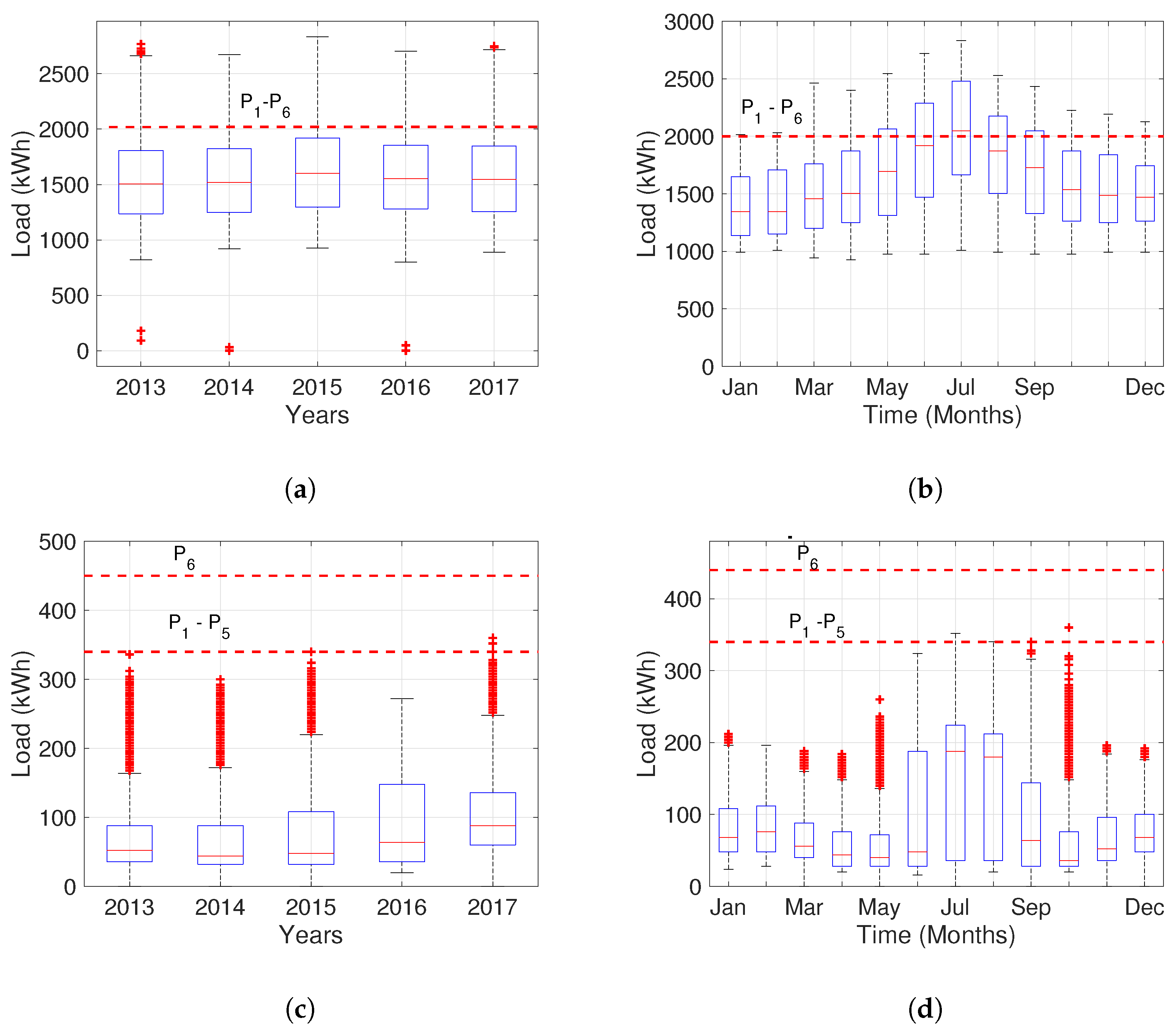
These datasets can be represented by their corresponding boxplots (Figure 1) and both contain quarter-hourly demand from 1 January 2013 to 1 December 2017. We notice, for the HUF case, that the demand exceeds the current power contracted level, in such a way that values above this limit are considered as overshoots of the demanding power and they causes penalties in the final price. For this case, the optimal set of power levels should be higher than the current ones. On the other hand, for CEA case, the load profile mainly remains below the limits indicated by the dashed lines, which suggests that the current contracted power levels were higher than the optimal.

The historical database contains 35,040 consumption registers by year with a sampling period of 15 minutes (i.e., 4 × 24 × 365 = 35,040 samples). These registers must be allocated by block (1–6) and by month, day, and hours (i.e., time block division for TOU pricing), as detailed in

Table 1. Six-block time division for the used time-of-use (TOU) rates in our data.

Block	Type A (Hours)	Type A1 (Hours)	Type B (Hours)	Type B1 (Hours)	Type C (Hours)	Type D (Hours)
1	10–13 18–21	11–19	-	-	-	-
2	8–10 13–18 21–24	8–11 19–24	-	-	-	-
3	-	-	9–15	16–22	-	-
4	-	-	8–9 15–24	8–16 22–24	-	-
5	-	-	-	-	8–24	-
6	0–8	0–8	0–8	0–8	0–8	0–24
Mon-Fri	1	1	1	1	1	0
Sat-Sun	0	0	0	0	0	1
Holidays	0	0	0	0	0	1
Months	1,2,12	6 ${}^1$,7	6 ${}^2$,9	3,11	4,5,11	1,…,12

${}^1$ Second half of the sixth month; ${}^2$ First half of the sixth month.

.

4. Experimental Results

In this section, we analyze the results obtained when applying the proposed methodology to the available databases from the HUF and CEA buildings. The optimization problems were solved using Matlab-based CVX software (version 2.1, CVX Research, Inc., Austin, TX, USA) for convex optimization [27]. First, we present the results of evaluating the function cost when the optimal set of power levels is applied. Then, we present the results of data processing followed to determine the sensitivity description, which basically consisted of performing bootstrap resampling from the LM for every pair of months and TOU block. Finally, we analyze the sets of sensitivities in terms of the introduced mosaic representations, showing that they allow us to readily identify where the optimization constraints and demand need to be focused to adopt DR mechanisms in a TOU scenario.

4.1. Cost Analysis in Terms of the Optimal Power Level

The upper part of

Table 2. Power levels and results of cost evaluation.

Building	Year	Optimal Power by Period		Cost (€/year)		Savings %
		${\mathit{t}}_{1-5}$ (kW)	${\mathit{t}}_6$ (kW)	Current	Optimal
HUF	2017	2168	2168	251,784	247,229	1.81
	2016	2126	2269	250,589	251,160	−0.22
	2015	2318	2318	278,540	270,570	2.86
	2014	2125	2200	249,552	246,142	1.37
	2013	2197	2197	257,287	-	-
CEA	2017	208	450	16,983	13,997	17.58
	2016	238	450	16,956	13,366	21.17
	2015	261	450	16,956	15,700	7.41
	2014	206	450	16,956	12,312	27.39
	2013	219	450	16,956	-	-

presents the optimal power set found by the proposed optimization method for the HUF and CEA cases in every analyzed year. With this approach, the optimal set of power levels calculated in the current year are the recommended ones to be contracted with the power supplier during the next year. According to the HUF demand profile, depicted in Figure 1a,b, these results confirm that the optimal set of powers should be higher than the current one, and they tend to stabilize in 2016 with the values in 2014. The table also shows how the optimized levels in the HUF, presented for the current year, affect the annual cost if they are applied to the next year (e.g., optimal power calculated with 2013 demand is applied to calculate the cost with 2014 demand). We obtained a saving metric for this evaluation when compared with their corresponding current cost by year. Moderate savings (max 2.86%) indicate that the current contracted power levels are close to the optimal. In this case, the DR strategy suggest that it is possible and recommendable to increase the power to be contracted during the next year.

For the CEA healthcare building, a different behavior was observed compared with the HUF, as in this case, the optimal set of powers are located below the current ones (see Table 2, lower part). Whereas the relative savings are apparently higher (max 27.39%), the amounts are noticeably much smaller. It can be seen that the optimum remains in general stabilized, except for the increment observed in 2015. There is a trend on the forward prediction to yield a slight overcost in the last three years, which was due to the fact that a change in the management was followed in which the building required to be increasingly cooled in the summer, which caused a change in the dynamics and a non-stationary modification on the conditions. However, the method is capable of providing a closer-to-the-optimum estimation.

In both cases, we see that several quantitative advantages can be obtained. Rather than the impact on the savings, this shows evidence that the consumption dynamics are being adequately captured by the optimization procedure. Accordingly, and rather than just giving a recommendation for the next-year tariff to contract, it seems desirable to provide information on these changes in the dynamics from one year to another, so that this information can be handled by healthcare building managers, as described next.

4.2. Overshoot, Lagrange Multipliers and Bootstrap

When formulating the optimization problem, one of our decisions was to consider the power excess (overshoot) as an explicit variable and to relate this variable to the power demand and the contracted power using a constraint. Such a decision brings two benefits: (i) the LMs associated with the constraint capture the sensibility of the cost in the objective to variations (uncertainties) on the demand; and (ii) we can rely on dual theory and sensitivity analysis to characterize those LMs. In this section, we evaluate the value of those LMs and use the results to asses the sensitivity to overshoots for every block and period.

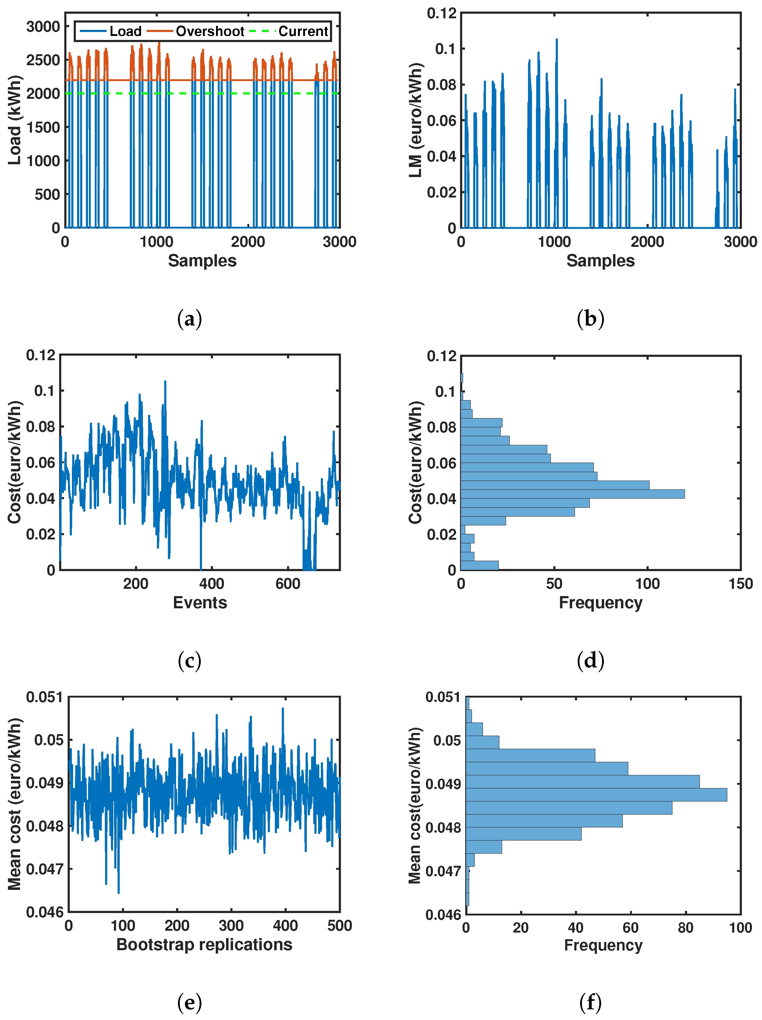
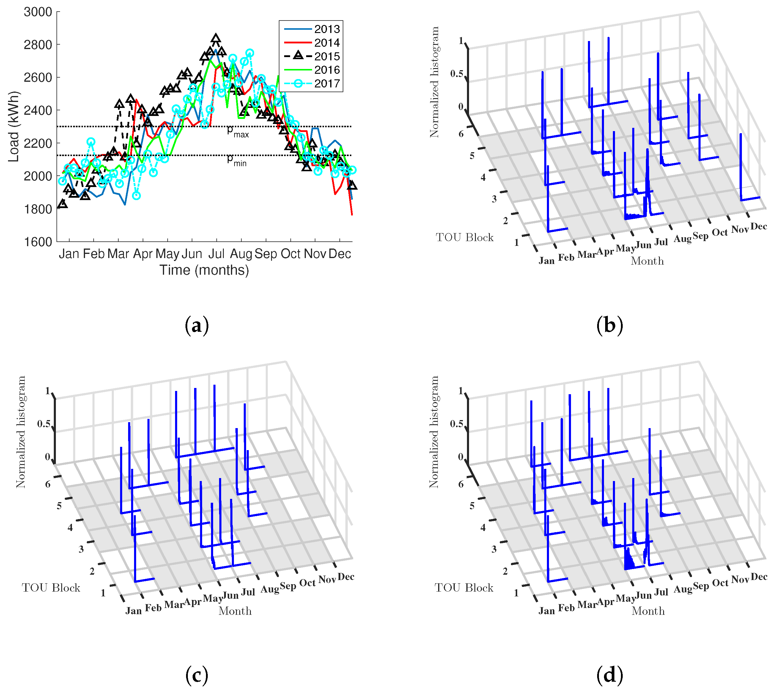
For the HUF case, Figure 2 shows an example of post-optimization data treatment allowing us to obtain the mean bootstrap sensitivity value and its distribution from the LM analysis. In Figure 2a, we can observe the load profile and the time instants when it overpasses the power limit. Note that the green dashed line depicts the current power level and the red line shows the overshoot with respect the optimal level. Figure 2b depicts the corresponding LM provided by the optimization algorithm output as a function of the same time instants, where it is clear that these LM track the overshoot with their instantaneous values, whereas these values remain at zero level with no overshoot. Figure 2c shows every overshoot as discrete variable that is active only for the specific $(t,m)$ constraint (i.e., block, month) defined in Equation (3). In the histogram in Figure 2d, the empirical PDF is represented for this price evolution, and the presence of complex shapes can be appreciated, as given in this case by bi-modalities. Figure 2e shows the average-values for every bootstrap replication, together with Figure 2f depicting its empirical PDF. Whereas the statistical distribution of the bootstrap-estimated values still includes the information of the overshoots that take place at every resample, its statistical distribution is not so affected by specific peaks happening in a specific realization. This provides a robust set of estimators, which are less affected by atypical samples, while respecting the impact of the overshoots on the statistical distribution description.

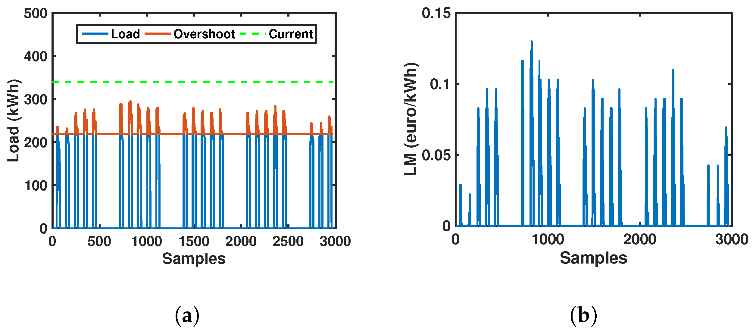
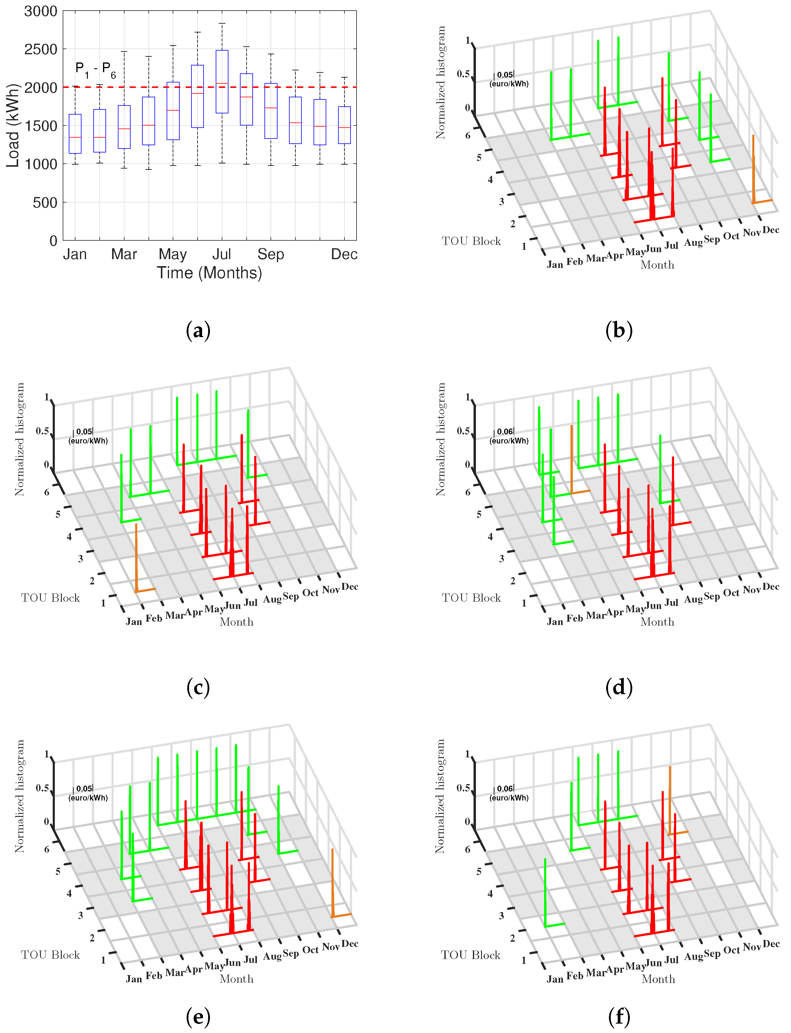
For the CEA case, the counterpart to Figure 2 is shown in Figure 3. Load consumption and the time instants when it overshoots the optimal power limit (red line) are shown in Figure 3a. Note that, for the currently contracted level (green dashed line), we can see that the optimal level is well below the contracted one, which in this case implies that in the equilibrium point it is preferable to allow some overshoots. LMs and their discrete representation are shown in Figure 3b,c, respectively. In the PDF distribution shown in Figure 3d, we observe a different distribution profile compared with the HUF case for these same conditions, where it is noticeable a trend to zero value. 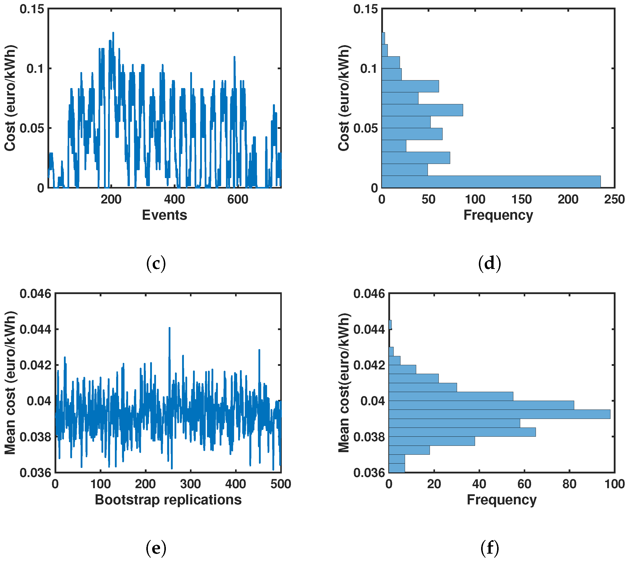Finally, in Figure 3e,f, the average values by bootstrap replication and its bootstrap distribution are shown, respectively. These statistical profiles are much alike the ones in the HUF case example, and again, they are including the information about the overshoots for the optimized problems, hence it represents a robust statistical measurement and characterization of the dynamics, which in turn can be readily compared with other situations. Hence, the use of sensitivity analysis in combination with bootstrap resampling yields a unified and robust representation of the underlying dynamics, which is subsequently analyzed in the next subsection.

4.3. Mosaic-Distribution and Sensitivity Results

We addressed the representation of mosaic distributions for the data from the available years (i.e., 2013–2017) according to Algorithm 1. Recall that, in the mosaic distributions for the LM empirical distributions, in horizontal plane, blank cells represent a distribution which demand do not overshoot optimal power level, and grey cells indicate that the corresponding month does not match with any TOU block. In addition, in the mosaic distributions for the bootstrap sensitivity analysis, blank cells represent a distribution whose CI overlaps zero and then it is not statistically significant, and hence, that distribution is not represented in the mosaic. Recall also that the estimated PDFs of the LM are depicted with green, orange, and red color when their corresponding average is low, moderate, and high, respectively.

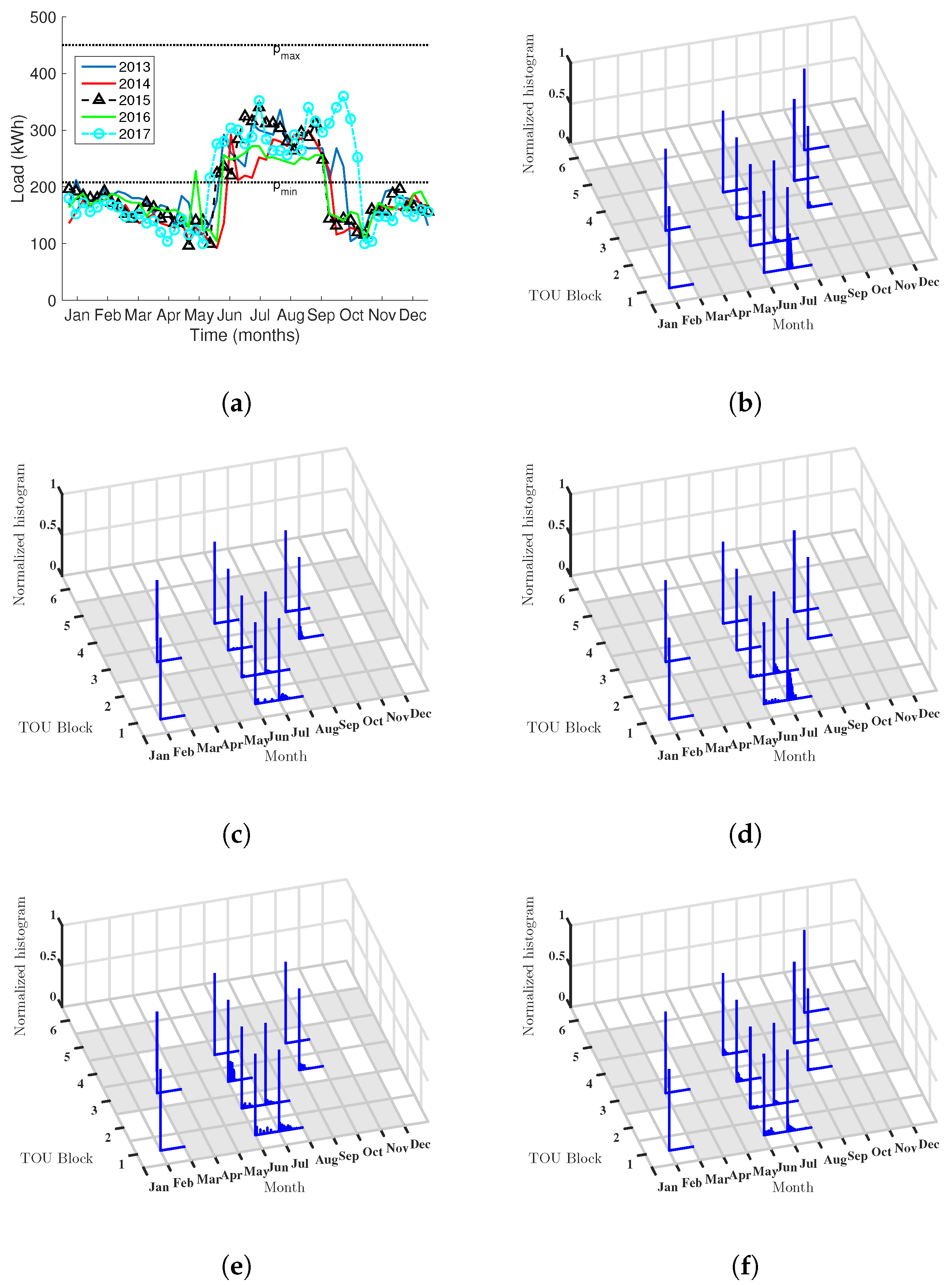
Figure 4 shows the mosaic distribution for the LM empirical distributions in the HUF case. The peak load is represented for each year in Figure 4a, so that we can have a view of the consumption profile. We can observe that the load overshoots the $p_{min}$ and even $p_{max}$ optimal power levels, which are identified by the dotted lines therein.

In Figure 4, those tiles whose 95% CI overlaps zero have been removed from the representation; nevertheless, most of the distributions are significantly present with this criterion. It can be also seen in Figure 4b–f that there is a noticeable bimodality and heavy tails in the distributions of the LM, which is just due to the threshold effect on the LM. This representation makes hard to identify which are the more crucial periods and months, and not much difference can be observed from one year to another.

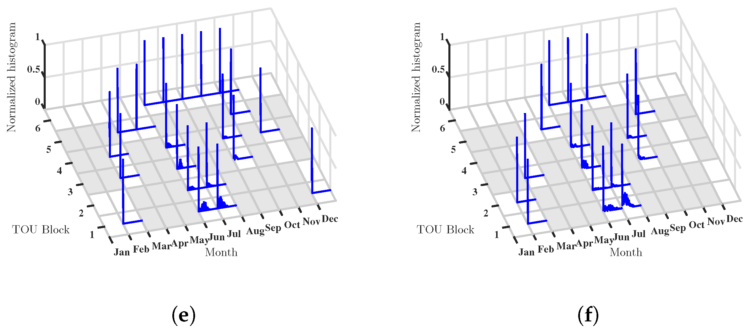
Conversely, Figure 5 shows the mosaic distributions for the bootstrap estimated averages. It can be clearly seen that distributions in red have clearly higher values, and more, there are temporal trends that can be observed through years. For instance, the red distributions are mostly grouped on the months of June, July, and September, for periods 1 to 4, and mostly repeated with minor changes. However, there is a trend in the red distributions following an inverted-U shape, which are more present in 2013 for the ending months, then they trend to reduce in those months but to increase in March and April during 2014 and 2015, and finally to be less evident in 2017. Hence, two sets of policies need to be separately considered, one for the summer, and another for the winter, which will be obviously different, but can be scrutinized in terms of what happened in those specific months in the observed years.

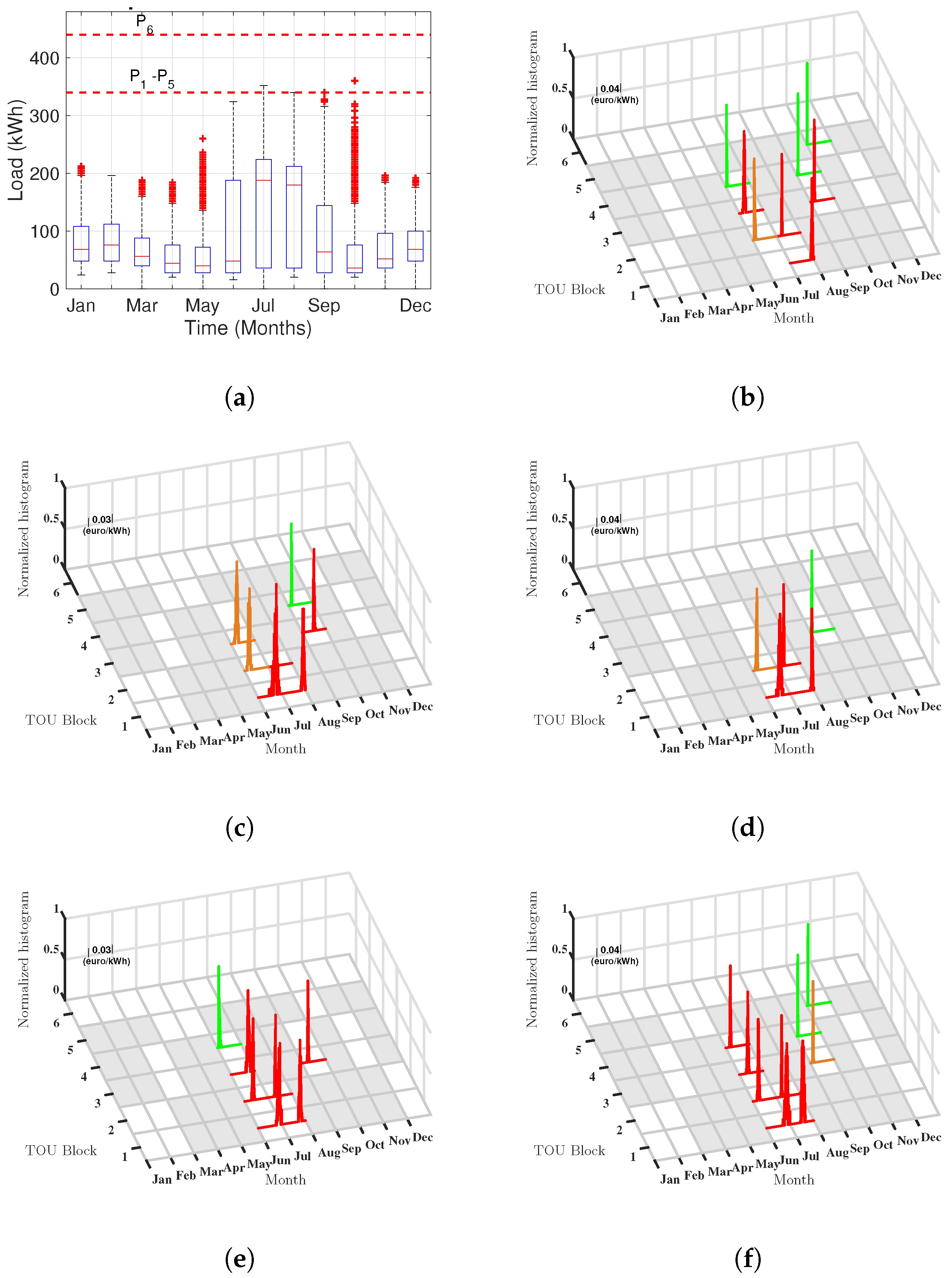
Different dynamics are observed in CEA. Figure 6 shows the peak load with a very different profile from the triangular trend in HUF, and, in this case, there is a flat trend in the summer months, probably related with the cooling air connection, and then a peak-trend with maximum in January but linearly decreasing, corresponding to the Winter months. In this case, the mosaic distribution for the LM empirical distributions has a different profile from the HUF distribution, and more, it remains stable and repeated through years. However, as seen in Figure 7, the mosaic representations for the bootstrap sensitivity analysis is very different from stationary. The U-shape set of significant green distributions is not present here, whereas the significant sensitivity is now condensed in the months of June, July, and September, being non-significant the other tiles. Nevertheless, the relevance of the significant tiles changes from one year to another, with a trend to increase the sensibility during years 2015 and 2017. These were the years where the policies on the air-conditioned management changes, and this trend is detected within this analysis to change the impact on the mosaic distribution. In

Table 3. Summary of maximum sensitivity by year.

Building	Max. Sensitivity (€/kWh)					Overall (€/kWh)
	2013	2014	2015	2016	2017
HUF	0.05	0.05	0.06	0.05	0.06	0.06
CEA	0.04	0.03	0.04	0.03	0.04	0.04

, we summarize the maximum sensitivity values obtained for CEA and HUF. In both cases, the maximum corresponds to 2015 and 2017 years.

5. Discussion and Conclusions

In this paper, we have proposed a twofold application of convex optimization to support managers of healthcare buildings in adopting a time-of-use based demand response program (DR-TOU). First, a simple yet novel method has been proposed which has been solved using convex programming tools. The analyzed scenario corresponds to the five years of data consumption available from two different sized healthcare buildings and the rate scheme to a six-block TOU pricing. Second, we provided the managers with additional information about the most relevant constraints to be paid attention, and, for this purpose, the statistical distribution of the constraint sensitivity of the time periods and pricing levels was scrutinized, giving a good view of which are the most critical of them on a new, systematic, and easy-to-handle representation with the so-called mosaic distributions.

Sensitivity analysis has been shown to identify at a glance where and when the interventions will be more urgent and more necessary to reduce the cost. The use of statistical tests based on nonparametric bootstrap resampling makes this instrument more than a visualization tool, and is solidly based on the statistical distribution analysis. The application of this method in two very different cases of study (different healthcare buildings) highlights the effective convenience and usability of this approach.

In our results, the analysis of the resulting optimization showed a cost reduction in the electricity bill of up to 27.81% per year, obtained in the smaller building with conventional energy management strategy. Clearly, it should not be used as an autonomous and isolated prediction tool, but rather as a support to the deep knowledge of the managers in their field. The statistical profiles in the distributions of the raw LM was shown to have limited information, whereas the profiles given by bootstrap resampling provided with useful and operative information about the dynamics and the most convenient tiles to scrutinize in order to manage the cost. Thus, the mean sensitivity of 0.06 €/kWh (for the larger building) and 0.04 €/kWh (for the the smaller building) could be a useful evaluation metric for those energy saving measures that require investment, finance viability and payback time (e.g., to invest in battery energy storage systems (BESS)). It can be concluded that the proposed novel system can be useful to determine the suitable power levels for the next year contract renewals, while giving a robust and operative overview of the optimized solution for DR-TOU management purposes. Finally, although our formulation is suitable for healthcare buildings, it could also be useful in other scenarios.