1. Introduction
Three-phase brushless drive systems, especially those based on permanent magnets motors, have proven to be a good solution for high efficiencies and compactness requirements. The three common types of brushless ac motors are synchronous reluctance (SynRM), non-salient permanent magnet and interior permanent magnet (IPM) ones (throughout this paper the last two will be abbreviated as permanent magnet synchronous motors—PMSMs). In addition, given the converter limits these motors, in particular the IPM type, also present the advantage of a wider constant power speed ratio (CPSR) which is desirable for operation above the corner speed, e.g., in traction applications. Brushless AC synchronous motors are designed using two common types of tools, numerical tools based on the finite element method (FEM) and analytical tools, and also combinations of both. Despite the large amount of simulation time required, FEM is the most adopted and preferred solution since it considers a multi-physics environment taking into account dependency of all parameters, e.g., cross-coupling, magnetic saturations and slotting effects, which may be neglected or assumed constant in analytical models. Analytical models based on the dq model are usually applied during the conceptual phase for initial sizing and when the performance behavior of the specific motor wants to be modeled typically for control purposes [
1,
2,
3].
The main drawback of FEM is its high computational cost, and the literature shows some practical solutions to reduce the simulation time by applying simplifying techniques limiting the number of simulation points [
4,
5,
6]. However, in any case there is a manual involvement of repetitive steps of the designer for performing simulations, exporting data, post-processing the data (usually with some other software tool, e.g., MATLAB) in order to compute specific performance points of the motor. These tasks can be tedious and time consuming, especially in the conceptual phase of the design where some parameters are usually still not defined (e.g., geometry, number of turns per phase, poles, slots, magnets, etc.) and only particular points are of interest to check whether the design meets a given requirement to consequently decide if changes are needed.
This paper is focused on developing fast algorithms to obtain the motor key operation points performance in order to compare a high set of machine candidates. For this purpose, different approaches were considered:
- -
Analytical sizing functions [
7,
8]: this approach is fast but not a high fidelity model. Then, it is possible that some discarded machines candidates could have better performance than the selected ones.
- -
Functions using reluctance based circuits [
9,
10]: this approach can reach satisfactory levels of precision, but any specific geometry will have a specific reluctance network. The time can be reduced, but when the precision is increased the complexity of the development of the network is increased and the computation time is also increased. A very high accurate reluctance circuit could finally require the same computation time as a FEM approach.
- -
FEM approach: it has high fidelity and any geometry can be directly studied [
1,
5]. The key design parameters are not directly obtained from FEM simulations. Additional equations should be added, and normally FEM simulations are done intensively and after interpolation functions are applied. These techniques are not adequate for a high iterative process with a high number of machine candidates.
The goal of this paper is to develop new functions that reduce the time needed to obtain the key performance operation points of any candidate machine for a future iterative design function. Nowadays, we have computers capable of making large amount of data computations that have resulted in the availability of several commercial FEM tools. Most of them offer the possibility to code within the tool to automate tasks. We take advantage of that fact and offer nine simple algorithms as an alternative for the evaluation of electromagnetic operation points in motor models in FEM within acceptable computation times of around twenty minutes for complex tasks such as obtaining the CPSR of the motor for given converter limits and below five minutes for simpler calculations such as the maximum torque for a given current. The algorithms apply three numerical approximation methods, Newton’s method, secant method and a curve fitting natural cubic spline interpolation. The convergence of these methods applied in the algorithms have been well studied in the past [
11,
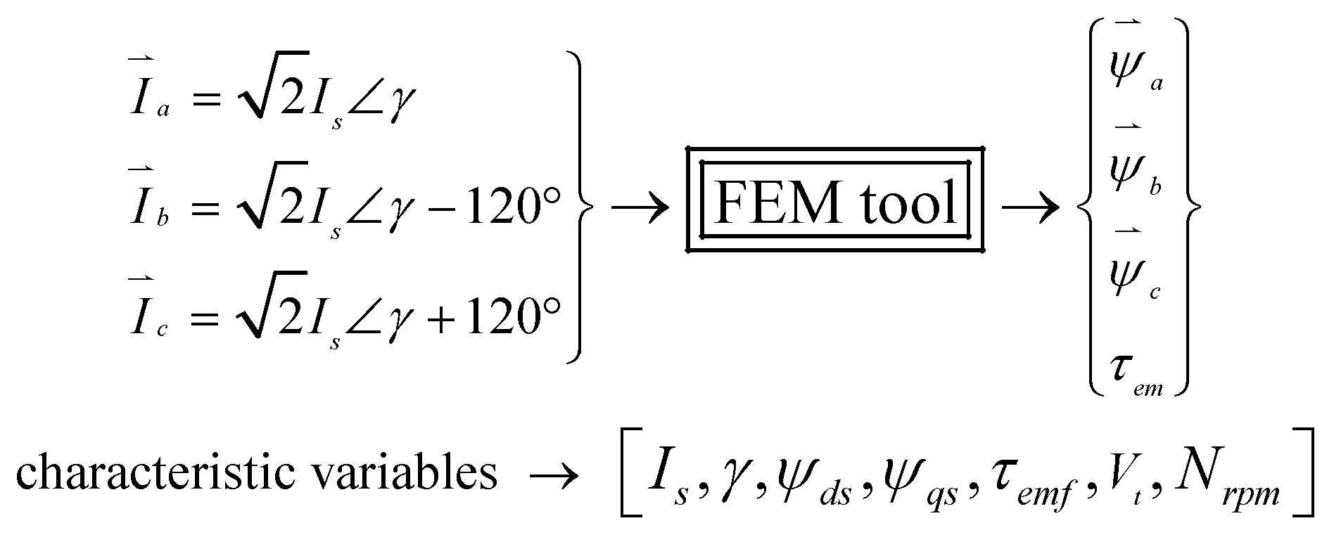
12]. The algorithms presented in this paper were developed with the objective of finding specific characteristic motor points of interest during the design process or during control design that cannot be targeted directly with a FEM tool such as maximum torque per Ampere (MTPA), minimum Ampere per torque (MAPT), maximum torque per voltage (MTPV), the speed for a voltage and current limit, characteristic or short circuit current (
Ich), the maximum power point during flux weakening, the CPSR and the boundary transition point from FW to MTPV control. Their logic intention was developed to work for the three types of brushless AC motor obtaining reliable approximations with the least number of simulation step points and iterations possible, therefore, in shorter times compared to a full simulation process, yet still flexible as to whether or not more steps are needed. A module with the algorithms was developed in Jython, which is the language in Altair Flux2D, the FEM tool used in this paper. Validation of the algorithms is done by the results obtained for three already validated motor model designs, a non-salient permanent magnet motor, an IPM and a SynRM [
13]. The results are compared with the reference values of each motor and the time of execution in seconds for specific inputs are shown.
The remainder of this paper is organized as follows:
Section 2 overviews the related theory for the application of the algorithms. The proposed algorithms are presented in
Section 3.
Section 4 presents a use case example to compare the computational time by a typical process to obtain a motor characteristic and the process using the algorithms.
Section 5 is the validation section where the speed characteristics results for the three types of brushless motors are computed with the algorithms and compared with its reference value. Finally,
Section 6 concludes the paper.
3. The Proposed Algorithms
In order to execute the proposed algorithms some auxiliary functions will be necessary, however, these depend upon the specific FEM tool commands or are well known algorithms. Therefore, to make it short and simple, in this paper some steps within the algorithms will be only mentioned as processes and the developer must adjust the tool to execute these respective processes. Among these functions are Park’s transformation, cubic spline interpolation algorithm, and automatic simulation of a point on the FEM tool. In addition, some inputs depend on the motor model e.g., pole pair number, initial alignment angle, phase resistance, etc. and others are specific of the FEM tool e.g., the name given to parameters, step number, initial position, etc., henceforth, other inputs not mentioned for the specific model and tool are called motor model and tool parameters.
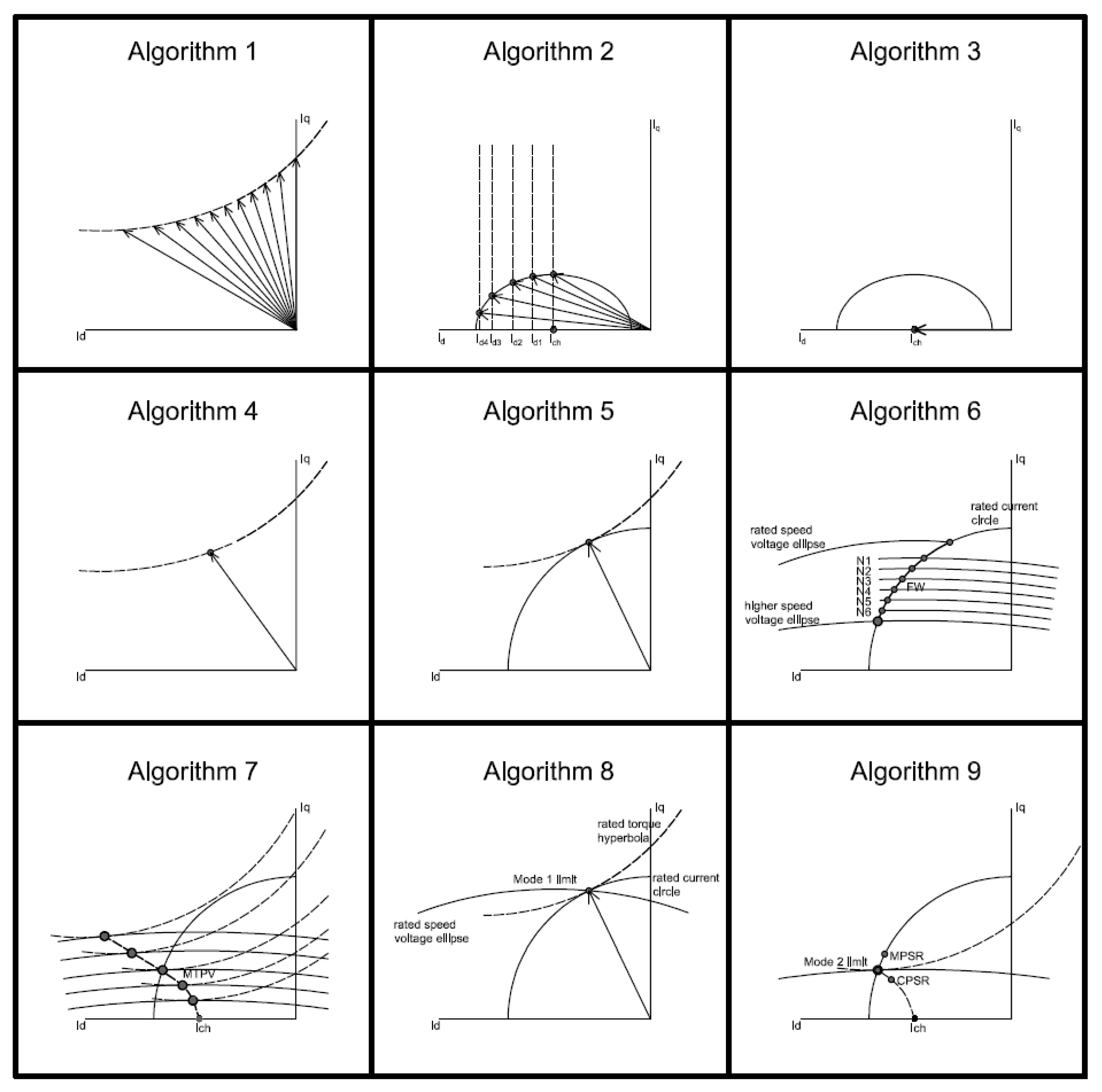
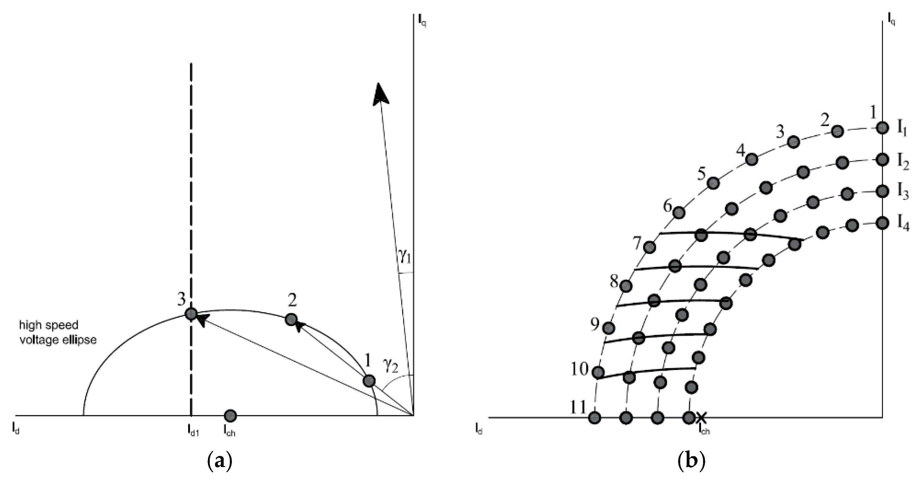
Figure 3 illustrates how each algorithm works and what operation points it can compute on the circle diagram. The objective of Algorithm 1 is to determine the targeted current magnitude for a given torque and a fixed angle value, in this case the secant method is used to converge to the result, and usually it finds the value in less than ten iterations if the first guessed is not too far. In a similar way using the secant method, Algorithm 2’s objective is to determine the characteristic variables for a given voltage value for a fixed
Id. In this case, the angle
is parametrized with a fixed
Id current to avoid divergence of the algorithm. This is better explained with
Figure 4a, if the voltage ellipse is small i.e., for a high speed, the algorithm may diverge if the angle is not correctly targeted, for example for
there is no convergence to the given voltage and speed, for
depending on the initial guess the algorithm may converge to point 1 or 2. Therefore, in order to have a sort of control an
Id current is fixed, having iterations only in
Iq until convergence e.g., point 3, otherwise we are outside of the voltage ellipse. For both algorithms to compute the derivative approximation in the secant method two first guesses are needed in this case zero was given as one initial value for the torque and current since it is a known point, however, this may be changed or the algorithm may be adjusted to compute two initial guesses.
| Algorithm 1. Given the torque and angle get the current magnitude that produces that torque |
| 1: Given , , tolerance > 0, k: = 0, kmax, initial , step_number = n, motor model and tool parameters |
| 2: Initialize variables = [0]; = [0]; converge = False |
| 3: While not converge: |
| 4: simulate point (,) with given step_number |
| 5: get |
| 6: compute , |
| 7: compute with Equation (3); |
| 8: append values to and |
| 9: If : |
| 10: converge = True |
| 11: return(characteristic variables) |
| 12: elif k = kmax: break |
| 13: else: |
| 14: ; |
| 15: |
| 16: k = k + 1 |
| Algorithm 2. Given the speed, voltage and Id current get the characteristic variables where the voltage is reached |
| 1: Given , , tolerance > 0, , k: = 0, kmax, initial , step_number = n, model and tool parameters |
| 2: Initialize variables = [0]; = [0]; converge = False |
| 3: While not converge: |
| 4: compute with Equation (4) |
| 5: compute with atan(/) |
| 6: simulate point (,) |
| 7: get and compute , |
| 8: compute with Equation (1) |
| 9: append values to and |
| 10: If : |
| 11: converge=True; compute |
| 12: return(characteristic variables) |
| 13: elif k = kmax: break |
| 14: else: |
| 15: ; |
| 16: |
| 17: k = k + 1 |
Using the secant method in Algorithm 3 we get Ich based on Equation (2) when solved for Id. Ich is the value of Id needed to drive to zero. An initial value of one was given to flux d to avoid zero division error, this can be changed by computing two initial guesses or give the magnet flux if known for the PMSMs. In Algorithm 4 we target the value of the MAPT point for a given torque, in summary what is done is to compute the constant torque curve for different angles using Algorithm 1, then using cubic spline interpolation obtain the minimum current magnitude. The MAPT point is basically the same MTPA point but targeted with the torque instead of the current.
| Algorithm 3. Get Ich of the motor |
| 1: Given tolerance > 0, initial , k: = 0, kmax, step_number = n, model and tool parameters |
| 2: Initialize variables = [0]; = [0]; = [1]; converge = False |
| 3: While not converge: |
| 4: simulate point (, 90) |
| 5: get and compute append results in , , |
| 6: If : |
| 7: converge=True; compute |
| 8: return(characteristic variables) |
| 9: elif k = kmax: break |
| 10: else: |
| 11: ; |
| 12: |
| 13: k = k + 1 |
| Algorithm 4. Given the torque get the MAPT point |
| 1: Given , tolerance > 0, , where , initial , k: = 0, step_number = n, motor model and tool parameters |
| 2: Initialize variables = []; = []; = []; = []; = []; |
| 3: For each value in run Algorithm 1 with |
| 4: Append results in , , , , |
| 5: Stop when |
| 6: Optional. After stop apply bisection as needed between and for a better approximation, particularly when steps in are large. |
| 7: Apply cubic spline interpolation to variables , , , , |
| 8: Get min() and its index |
| 9: Get the rest of variables at that index. |
| 10: Compute with Equation (1) |
| 11: return(characteristic variables) |
In Algorithm 5 we target the MTPA point for a given current, which is a simple process of sweeping different angles for the same current magnitude, then using cubic spline interpolation obtain the maximum torque value and return the characteristic variables for that point. Algorithm 6 uses the Newton’s method to obtain the speed for a given voltage limit, in a specific current vector, the process is illustrated in
Figure 4b, for a current I
1 and a given set of angles 1 to 11 in the figure the algorithm finds the corresponding speed for the voltage limit for each point. In this case we need to compute the derivative of the voltage with respect to speed, this derivative is given in Equation (7). The MTPV point for a given speed and voltage limit is obtained through Algorithm 7, it uses Algorithm 2 for different
Id currents getting values along the voltage ellipse and finally uses cubic spline interpolation to find the maximum torque:
| Algorithm 5. Given the current limit get the MTPA point |
| 1: Given , , where , k: = 0, step_number = n, motor model and tool parameters |
| 2: Initialize variables = []; = []; = []; = []; |
| 3: For each value in simulate point(,), get and compute , , |
| 4: Append results in , , , |
| 5: Stop when |
| 6: Optional. After stop apply bisection as needed between and for a better approximation, particularly when steps in are large. |
| 7: Apply cubic spline interpolation to variables , , , |
| 8: Get max() and its index |
| 9: Get the rest of variables at that index |
| 10: Compute with Equation (1) |
| 11: return(characteristic variables) |
| Algorithm 6. Given the current and voltage limit get the FW speeds along the current circle |
| 1: Given , , tolerance > 0, initial , where , k:= 0, kmax, step_number = n, motor model and tool parameters |
| 2: Initialize variables = []; = []; = []; converge = False |
| 3: For each value in simulate point (,), get and compute , , |
| 4: Append results in , , |
| 5: For each item index i in : |
| 6: While not converge: |
| 7: compute with , [i], [i], [i] in Equation (4) |
| 8: If : |
| 9: converge = True; compute ; |
| 10: return(characteristic variables) |
| 11: elif k = kmax: break; |
| 12: else: |
| 13: compute with Equation (8) |
| 14: |
| 15: k = k + 1 |
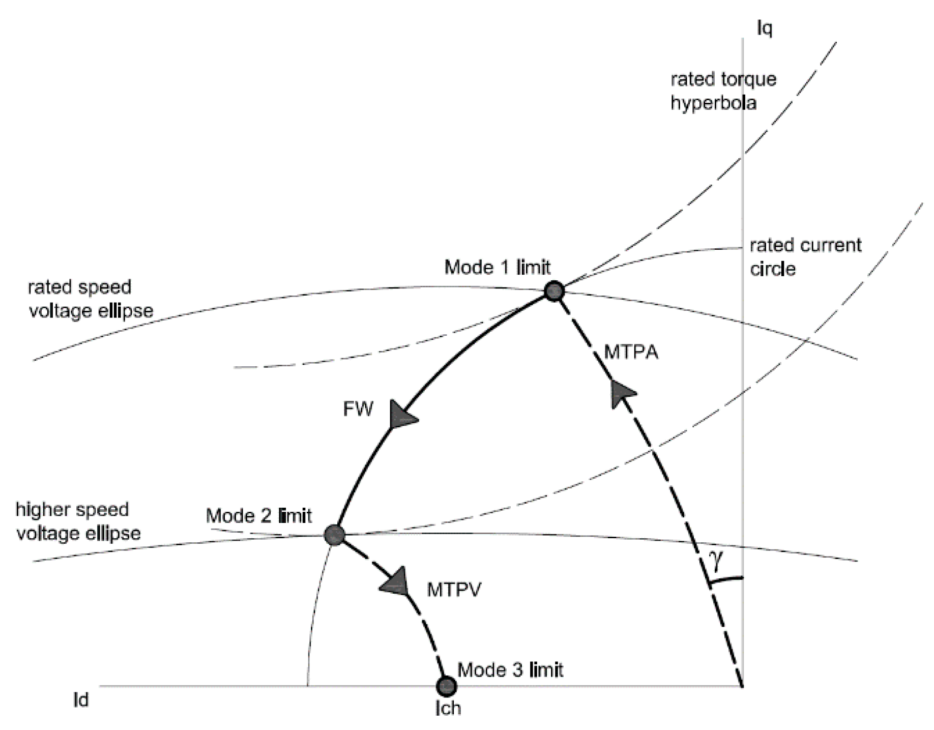
The objective of Algorithms 8 and 9 is to find mode 1 and 2 limit, respectively. Algorithm 8 assumes the limit is given by the voltage, it iterates along the MTPA curve using Algorithm 5 until the voltage is found as illustrated in
Figure 1, in this case we do not take into account the current or torque limit, the user criteria must decide if the point is valid or not. This was done because if the torque or current decide the limit then Algorithm 4 or Algorithm 5 can be used. Finally, Algorithm 9 finds the mode 2 limit, the CPSR and the MPSR point for the case where
Ich <
Imax because for the case where
Ich ≥
Imax a simpler analysis using Algorithm 6 can be done. These points can be found in different ways e.g., using Algorithm 7, however, its convergence is slower. Therefore, we use Algorithm 6 due to FEM tools simulate a working point targeted with phase currents, then, converging faster compared to any other way of iteration. The process can be explained with
Figure 4b, here we use Algorithm 6 for different currents
I1 to
I4 in this example, and then we automatically process the results using cubic spline interpolation to find different query speeds voltage ellipses (the solid lines crossing the currents) then applying interpolation to find the maximum torque on each ellipse, to finally find the limits of the motor.
| Algorithm 7. Given the speed and voltage limit what is the MTPV on the corresponding voltage ellipse |
| 1: Given , , tolerance > 0, where , k: = 0, kmax, step_number = n, motor model and tool parameters |
| 2: Initialize variables = []; = [], = []; = []; = []; Stop = False |
| 3: While not Stop: |
| 4: for each value in run Algorithm 2 |
| 5: append results in , , , , |
| 6: If : Stop=True; Optional. After stop apply bisection as needed between and for a better approximation, particularly when steps in are large. |
| 7: Apply cubic spline interpolation to variables ,, , , |
| 8: Get max() and its index |
| 9: Get the rest of variables at that index |
| 10: return(characteristic variables) |
| Algorithm 8. Given the voltage limit get mode 1 limit. |
| 1: Given , tolerance > 0, where , initial and , , k: = 0, kmax, step_number = n, motor model and tool parameters |
| 2: Initialize variables = []; = [], = []; = []; = []; = []; Stop = False |
| 3: Run Algorithm 5 for and |
| 4: Append results in , , , , , , stop if |
| 5: While not Stop: |
| 6: ; |
| 7: |
| 8: run Algorithm 5 append results in , , , , , |
| 9: If : |
| 10: Stop = True |
| 11: return(characteristic variables) |
| 12: elif k = kmax: break |
| 13: k = k + 1 |
| Algorithm 9. Given the voltage and current limit get the mode 2 limit, CPSR and MPSR. |
| 1: Given , , , where and , , , k: = 0, kmax, step_number = n, motor model and tool parameters. |
| 2: Initialize variables = []; = []; = []; = []; = []; = []; = []; = []; = []; = [], = [] |
| 3: create array where |
| 4: for each value in and for each run Algorithm 6 append results in , |
| 5: Apply cubic spline interpolation to ,, with more steps and append in , , |
| 6: create array where |
| 7: For each value in get vectors , for each by cubic spline interpolation using , , , |
| 8: For each speed in interpolate ,, with more steps |
| 9: get max() and its index |
| 10: get , , value at that index and append results in ,, |
| 11: Compute power with and append results in |
| 12: With , ,, , get mode 2 limit characteristic variables which is the highest speed at , get CPSR point and characteristic variables which is the highest speed where is equal to , if no value found then CPSR is infinite and get the MPSR point with the speed at the maximum point in . |
| 13: return (characteristic variables for mode 2 limit, CPSR and MPSR) |
4. Use Case Example and Process Comparison
One of the advantages the algorithms can provide is in the conceptual phase of the design, where changes to features of the model such as geometry is repetitive in order to find a valid model that can later be completely characterize.
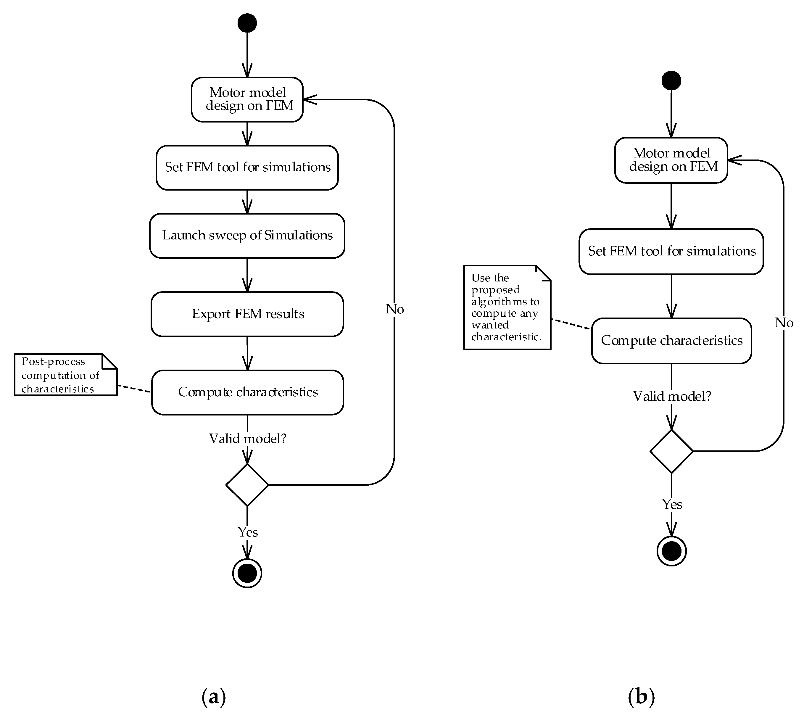
Figure 5a shows a typical process followed to compute a motor’s characteristics using FEM. Once the model is set and ready, a sweep of simulation points are done by introducing a range of three sinusoidal phase currents, the outputs are (but not limited to) fluxes, currents and electromagnetic torque. After the results are ready, usually the designer exports them for post-processing in order to obtain the characteristics that satisfies requirements and study the performance of the machine at different load points.
The algorithms provide an alternative to compute the motor characteristics within the same FEM tool. It is important to remark if the model design is already valid, the conventional process in
Figure 5a will allow to have the exported results at hand which will make the study of the performance of the motor easier. Then, the algorithms not intend to eliminate any valid design process but to provide an alternative of motor characteristics computation, in addition to help find answers faster when the need of the computation of one or more characteristics exist and the model is still not definite to be completely characterized.
Figure 5b shows the process using the algorithms that can be followed to check if the motor model is valid. As illustrated this can be done in two fewer steps compared to the typical process.
To compare the computation time consumption in both processes with similar conditions an example is now given with a ferrite IPM motor. For comparison only computation time is considered, not any human work time to develop a task is taken into account, although it is evident the conventional process involves more work. Suppose we have just finished a new IPM motor geometry design with the features mentioned in
Table 1. looking to satisfy the rated values specified in
Table 2. The best current phasor that will satisfy these requirements is of course on the MTPA curve. However, we do not know what that current phasor is. So with no prior analysis the current phasor will be found using both processes mentioned in
Figure 5. The application is set to magnetostatic 2D, the tool use is Flux 2D/3D from Altair, it has Jython as the coupled language.
The process “set FEM tool for simulations” only refers to prepare the model to execute simulations like faces, regions, mesh, physics, materials, etc. Because this is common for both processes the time in the comparison is not considered.
The sweep of simulations for the conventional process is launched with the following range of values, assuming the result lies between these values:
- (1)
Range to search the MTPA current angle: [5°, 65°] in 10 steps.
- (2)
Currents magnitude range for each angle: [8 A, 15 A] in 8 steps.
- (3)
Number of steps in one-sixth of the electrical period (position angle): 3.
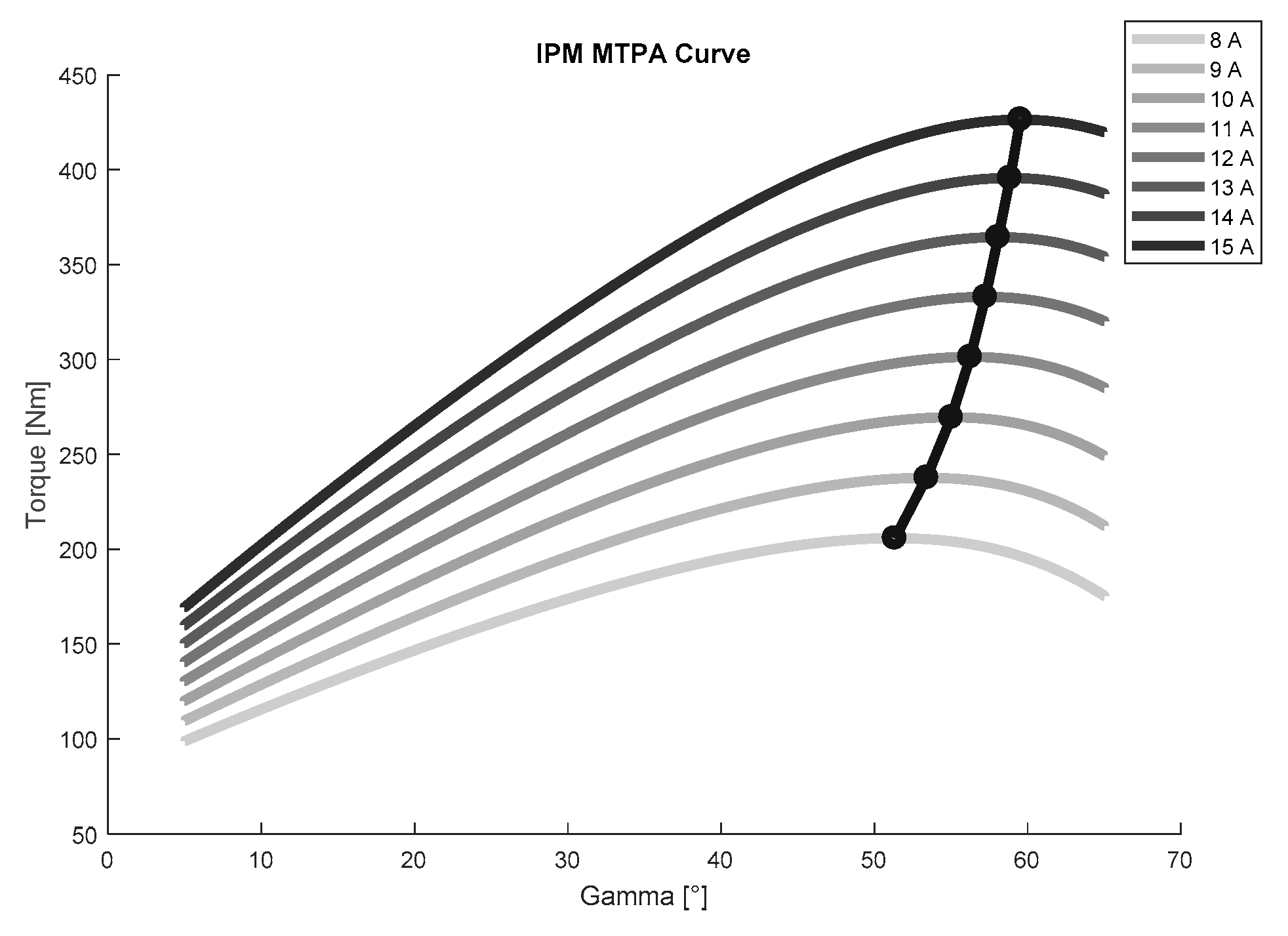
The time to finish the simulations was of 1457.37 s. The results were exported to excel, to be used in Matlab for post-processing. The time of exporting the results was of 91.02 s. Applying pre-developed post-processed scripts after the results are imported in Matlab the MTPA for each current is found as it is shown in
Figure 6. The computation time to find the current on the MTPA curve that satisfies the rated torque value was of 0.4315 s.
Now, for the process using the algorithms. Algorithm 4 computes the minimum current vector for a given torque value. For the reference torque of 370 Nm the algorithm inputs were set as follows:
- (1)
Torque tolerance 1 × 10⁻² Nm
- (2)
Current angle range [5°, 65°] in 10 steps.
- (3)
Current magnitude initial guess 10 A
- (4)
Number of steps in one-sixth of the electrical period (position angle): 3.
The process lasted a total of 1076.83 s. The current results for each process and the computation time consumption comparison are summarized in
Table 3.
The computation time results suggest that in similar conditions using the algorithms will give the advantage to the designer of reducing computational time to obtain a characteristic, besides less work to do it. The results show the current magnitude is above requirements then changes to the model must be made in order to satisfy them and the process should be repeated. If changes to the model are automated with scripts and the algorithms are used inside them, these provide the possibility to generate different machine candidates within the same FEM tool taking into account all multi-physics effects of FEM. This example was given with Algorithm 4 to compute the minimum current phasor for a given torque which is one of the algorithms that takes longer to give a result, nevertheless, Algorithms 1, 2, 3 and 6 are algorithms that usually take less than 5 min to provide an answer. The use and selection of the algorithms must be adjusted by the designer needs to get the most out of it. Validation of the algorithms is presented in the next section by computing the speed characteristics of the three typical brushless motors with already valid motor models designs.
5. Validation
To validate the algorithms the speed characteristics for the three types of brushless AC motors are computed. The motors here mentioned already have validated design models [
13]. General characteristics of the motors are mentioned in
Table 4, for the purpose of this paper the designs were intentionally modified in order to have their characteristic current (
Ich) below rated currents. The algorithms were developed in Jython and are implemented in the FEM tool Flux 2D/3D of Altair. The computer used is an Intel core i5-4590 CPU with 16 GB of RAM and the Windows 7–64 bits OS.
The process here undertaken consisted of computing the three limits of operation for each motor, some points on the MTPA, FW and MTPV curves, the CPSR and MPSR point, then, the results are plotted in order to show the circle diagram and speed characteristics for each motor. The mode 1, 2 and 3 limits are compared with its reference value and the time of execution in seconds of each algorithm are given, although this can vary depending the inputs of the algorithms and different factors of the motor model design. First, for all cases the model in the FEM tool is set to be control in polar mode as illustrated in
Figure 2, the simulations are set to be done in one-sixth of an electrical period in magnetostatic mode.
5.1. Selection of the Step Number
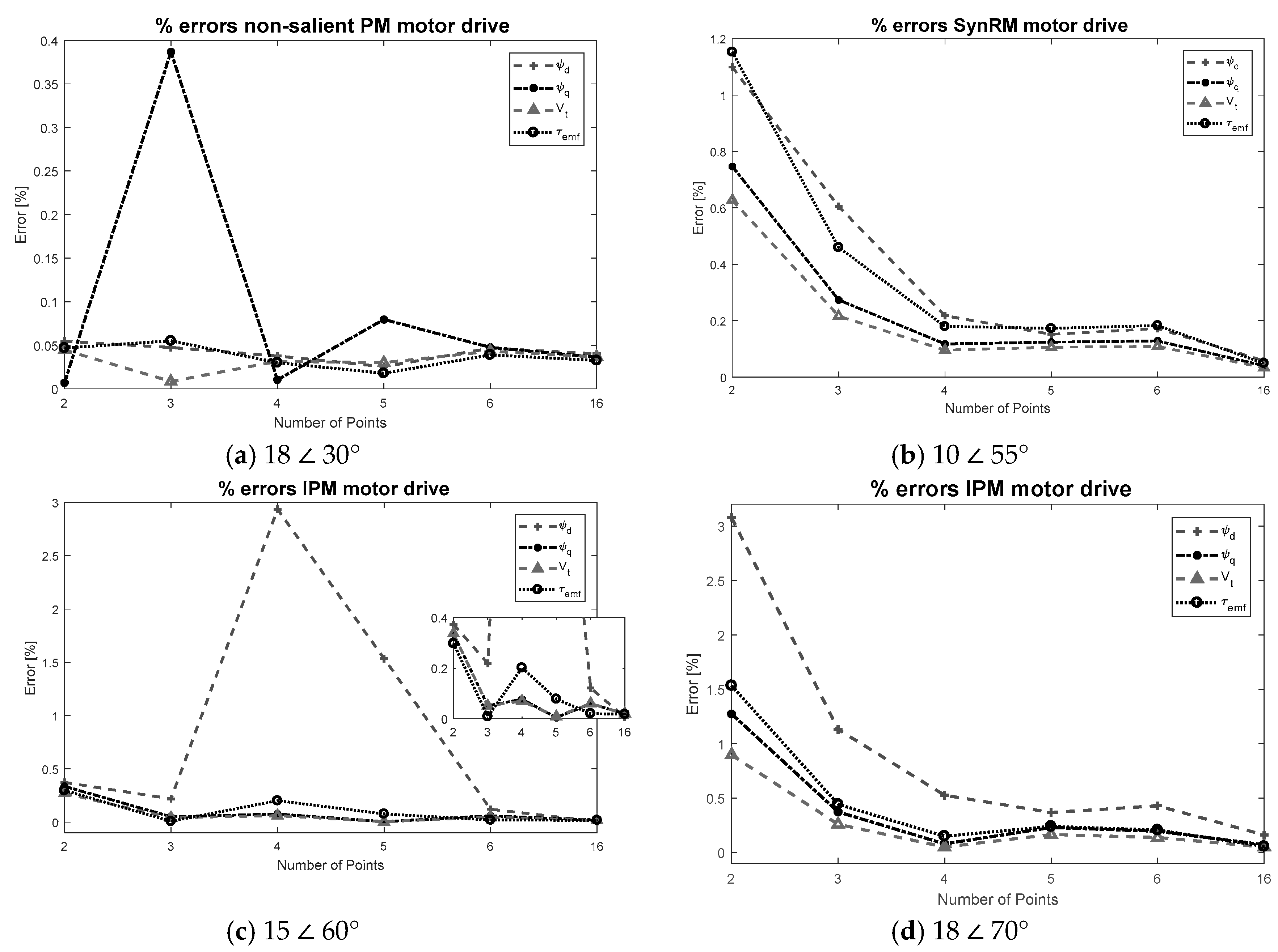
The selection of the step number may depend on the design factors of each motor model analyzed, therefore, it cannot be generalized. The designer should analyze and select the step number and length of the waveform to be studied for each motor case. Nevertheless, this subsection presents a numerical approach example on the selection of the step number for the algorithms. The algorithms are flexible and allow any number of steps to be introduced as well as the length of the waveform to be analyzed, however, the fewer steps introduced the faster its convergence. In this case, the selection of the step number is done based on a simple error analysis of the characteristic variables to check the amplitude of the errors we can make compared to a reference value by simulating with a reduced number of points. The error study was carried out for the three different brushless motor models.
This experiment consists of simulating a fixed operation point with two, three, four, five, six and sixteen step number points in one-sixth of an electrical period for mean values evaluation and compare the characteristic variable results with a reference value that is considered with adequate resolution. This reference value, in this case is selected to be 100 points in one electrical period since with this we assure that we can reach up to the 50th harmonic having at least two points per harmonic and for a mean value computation we considered it enough.
The motors are referred as the non-salient, the IPM and the SynRM motor.
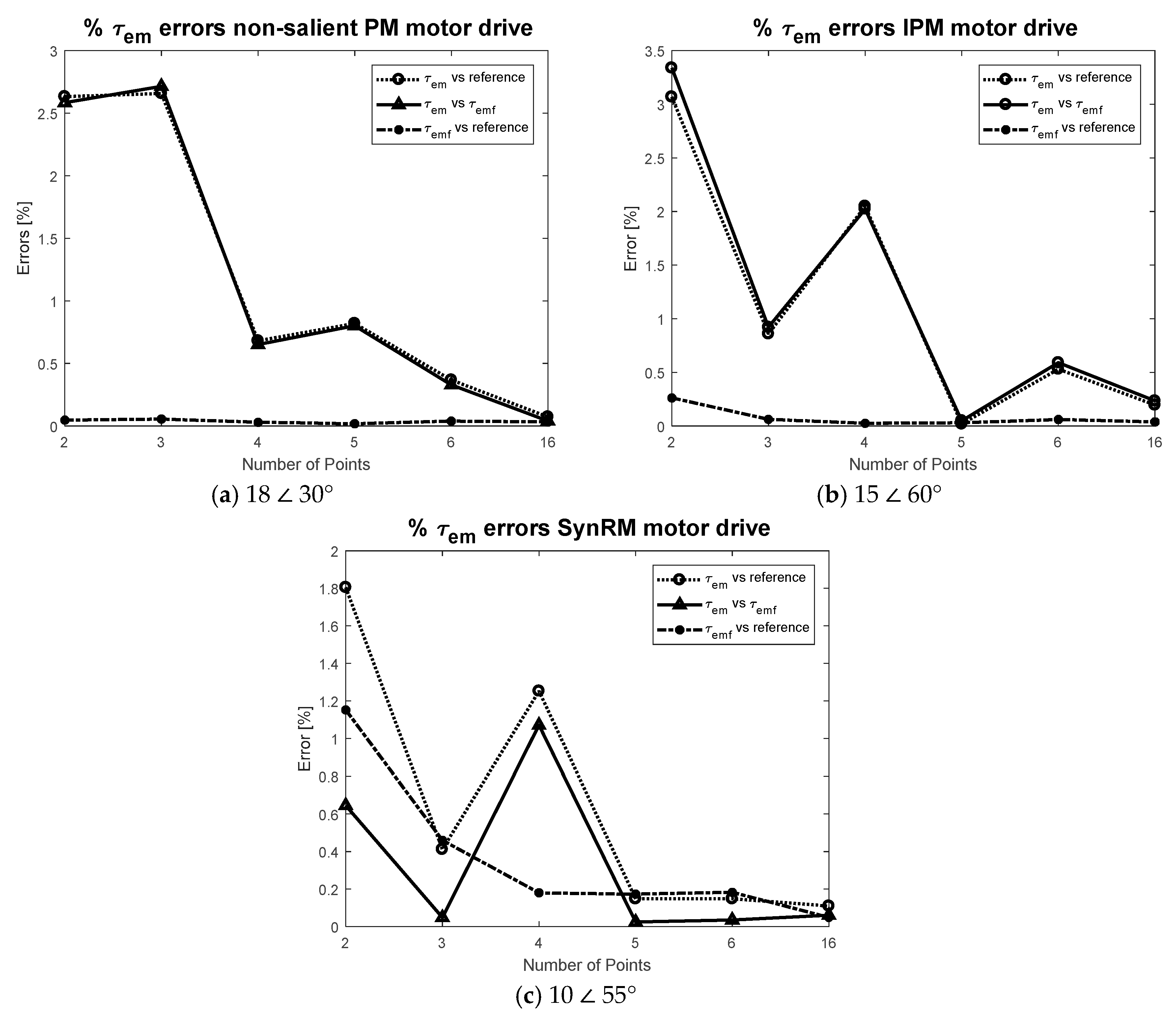
Figure 7 shows the torque errors for the three motors for a fixed current point.
is the obtained electromagnetic torque mean value directly from FEM results i.e., mean value of the output torque waveform for each specified step number. As mentioned in
Section 2,
is the torque computed with (3). It was found that the highest error occurs in
for a few number of points of simulation, which is expected since depending the torque ripple of each motor the mean value can be estimated wrong if the selection of the points are not carefully chosen. On the other hand, the error of
is smaller. It approximates the reference better, due to the flux linkage approximation of the waveform in one-sixth of the electrical period is better compared to the torque waveform approximation. Therefore, the reason to use the equations with dq fluxes for characteristics computation.
The errors for the characteristic variables of the three motor models are shown in
Figure 8. The errors for two different currents are illustrated in the same figure for the IPM motor with the purpose of showing that the error amplitudes are similar for different points of operation. Based on the results, knowing that for few number of points in one-sixth of an electric period the error found was below 5% for the three motors analyzed, as example, a step number of 2 for the non-salient motor, and a step number of 3 for the rest is selected.
5.2. Brushless Motors Speed Characteristics Computation
To find the speed characteristics the algorithms are applied as if having no or little knowledge of the motor behavior, e.g., we know that for a non-salient motor the MTPA curve is on the q axis (Id = 0), this could be computed faster with Algorithm 1 or Algorithm 2 depending the limit instead of applying Algorithm 8 another example is that Ich for the SynRM is zero and no algorithm is needed to find it, so no assumption is made and all points are found. This is done to show the time of execution of each algorithm in a worst-case scenario.
Table 5 shows the inputs applied to each algorithm listed in the order to compute the speed characteristics for the brushless machines. As aforementioned in
Section 5.1 we are using a 2 step number for the non-salient motor and 3 for the rest.
The time of execution in seconds as well as the number of iterations of convergence of each algorithm with the inputs aforementioned are presented in
Table 6. The large number of iterations for Algorithm 9 are due to Algorithm 6 which applies Newton’s method therefore most of the iterations are computed outside FEM. It can be noticed the time of execution varies depending the algorithm having the worst case for Algorithm 9 that takes 30 min to output the results. In general, the time of executions of each algorithm can be reduced by applying a better design criteria to the inputs, this is further explain in the next subsections.
The circle diagram and speed characteristic curves of each motor are now shown.
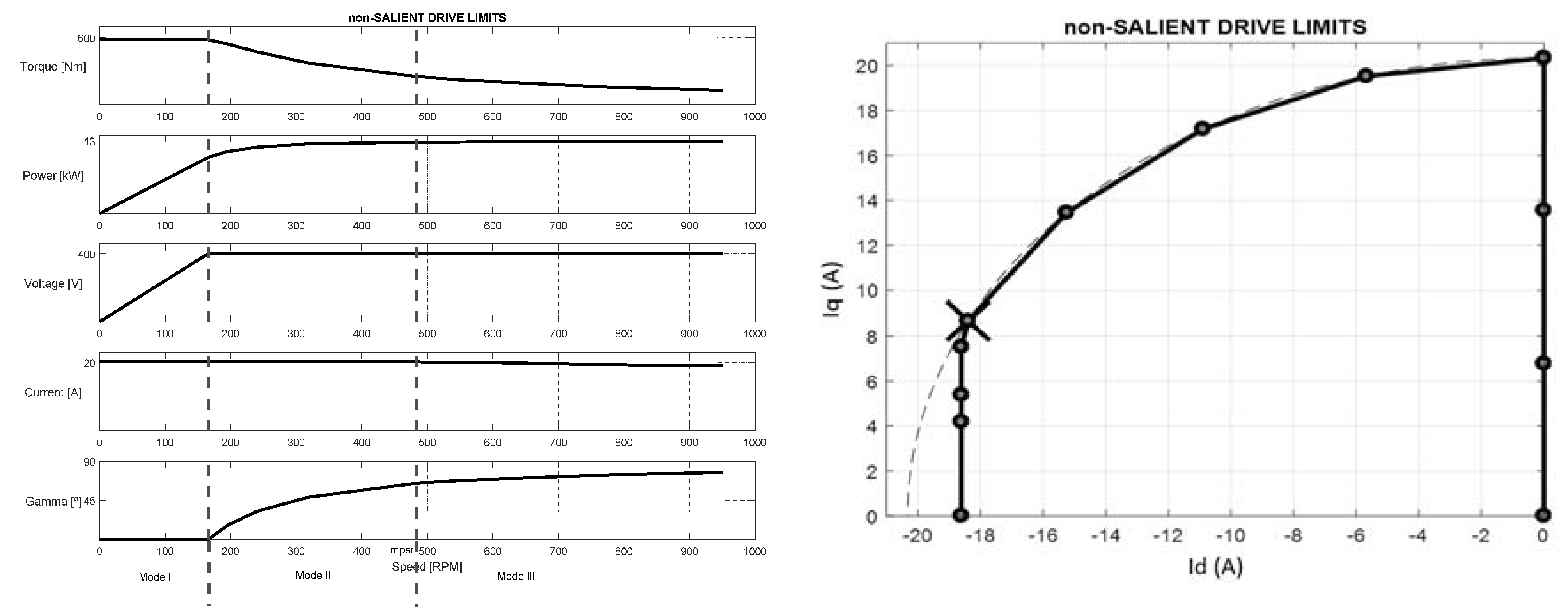
5.2.1. Non-Salient PM Drive
The non-salient PM is a 10 pole pair ferrite-magnet motor. The process to obtain the speed characteristic is the following. First, using Algorithm 3 the Ich is computed. Then, mode 1 limit is computed with Algorithm 8. Mode 2 limit, CPSR and MPSR points are computed using Algorithm 9, after this with Algorithm 6 two MTPA points below mode 1 limit are obtained. Finally, three speeds greater than mode 2 limit speed MTPV points are obtained with Algorithm 7.
Table 7 shows a comparison of the three different limits versus the reference value having the highest error of 2.1% in the mode 2 limit. Based on the authors’ experience the errors and time of execution are acceptable for practical purposes. Time can be reduced by applying the algorithms with better design criteria, e.g., for Algorithm 9, which has the longest time, depending the wanted precision the number of currents to be swept can be reduced as well as narrowing the angle vector (initial and end value) to be swept. All the results are plotted in
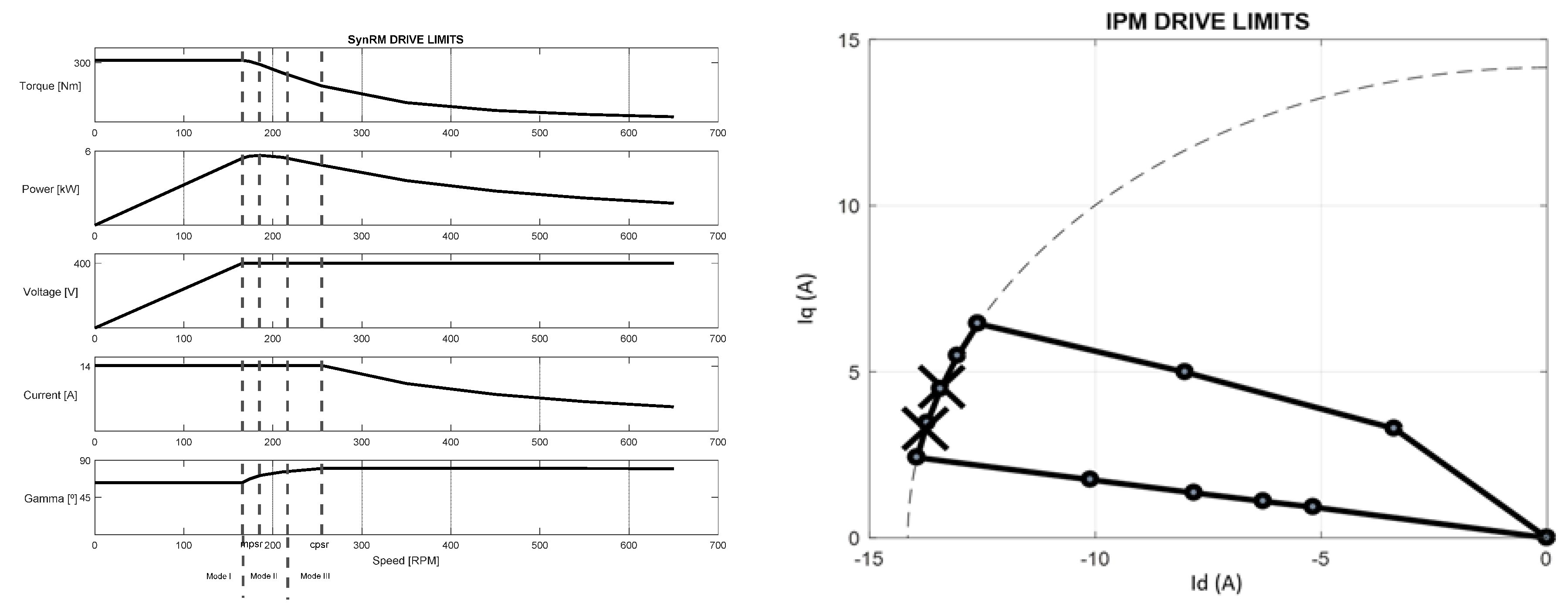
Figure 9, the limits of the different modes are marked with a dash line. In the circle diagram the MPSR is marked with an ‘X’. For this motor the CPSR is infinite and the MPSR is 2.91 found at the boundary point of FW and MTPV.
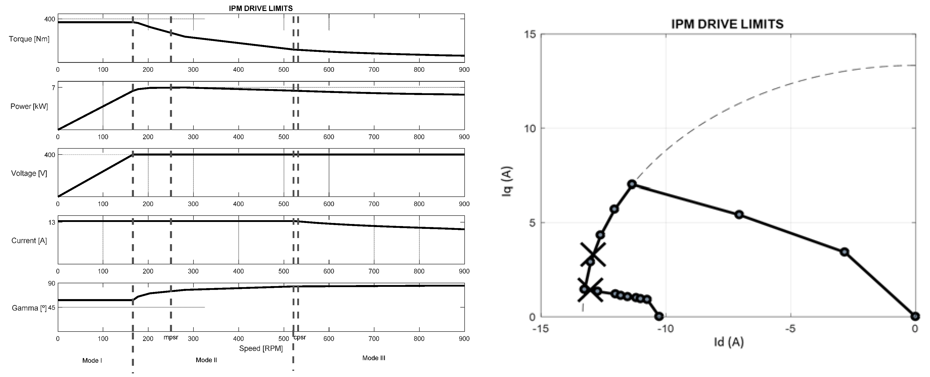
5.2.2. IPM Drive
The IPM is the same SynRM used in this paper with ferrite magnets in the slots of the rotor. The process carried out is the same as in
Section 5.1 with four more points computed on the MTPV curve.
Table 8 shows the comparison of the limits with the reference value. All computed points are shown in
Figure 10. On the circle diagram the MPSR and the CPSR points are marked with an ‘X’. The MPSR of this motor is 1.51 found in the mode 2 region and the CPSR is 3.2 found on the MTPV curve or in the mode 3 region, which is the expected behavior for an IPM.
5.2.3. SynRM Drive
The SynRM is a three pole pair motor. The process followed is the same as in
Section 5.1 with one more points computed on the MTPV curve.
Table 9 shows the comparison of the limits with the reference value. All computed points are shown in
Figure 11. The MPSR of this motor is 1.11 and the CPSR is 1.3 both found in the mode 2 region. On the circle diagram the MPSR and the CPSR points are marked with an ‘X’.
6. Conclusions
This work offers a set of algorithms coupled to FEM to compute typical brushless AC motor characteristics during the design process as an alternative to analytical models or repetitive post-processing tasks done after simulations. The algorithms take the advantage of the high fidelity non-linear electromagnetic environment of FEM tools to compute operation points such as MTPA, FW, MTPV and others that cannot be targeted directly, therefore, considering variable dependencies that are difficult to model analytically with high precision. A comparison of the conventional process and the process using the algorithms in similar conditions demonstrated the advantage of less computation time to obtain a motor characteristic with the proposed algorithms. The speed characteristics of a non-salient motor, IPM and SynRM were computed to validate the algorithms, the results were compared with a reference value having results under 3% error with two step simulations in one-sixth electrical period for the non-salient case, and three steps for the IPM and SynRM case. The time of execution in seconds was also presented taking around thirty minutes for the computation of mode1, and mode 2 limits, however, these can be reduced by applying better design criteria to the inputs. Finally, the results were plotted and the speed characteristics correspond to the expected behavior for the studied electric motors. Thus, validating the algorithms for the three typical brushless ac motors. It is considered that the developed algorithms will allow implementing global iterative design processes using directly a high fidelity electromagnetic FEM approach.


