Abstract
A novel method for Li-ion battery state of charge (SOC) estimation based on a super-twisting sliding mode observer (STSMO) is proposed in this paper. To design the STSMO, the state equation of a second-order RC equivalent circuit model (SRCECM) is derived to represent the dynamic behaviors of the Li-ion battery, and the model parameters are determined by the pulse current discharge approach. The convergence of the STSMO is proven by Lyapunov stability theory. The experiments under three different discharge profiles are conducted on the Li-ion battery. Through comparisons with a conventional sliding mode observer (CSMO) and adaptive extended Kalman filter (AEKF), the superiority of the proposed observer for SOC estimation is validated.
1. Introduction
Due to tremendous oil consumption and aggravated environmental pollution, electric vehicles (EVs) have exhibited great promise as a new, alternative means of transportation in upcoming decades [1]. EV performance is heavily reliant on the battery characteristics. Among various power batteries for EVs, such as lead–acid and nickel–hydrogen batteries, the Li-ion battery demonstrates its great superiority in terms of high capacity and power density, fast charge capability, long service life, no memory effect, and low self-charge [2].
The state of charge (SOC) reflects the remaining capacity of the battery and plays an important role in the battery management system (BMS) which guarantees the EV’s safety and reliable driving. In general, an accurate battery SOC indication is the foundation of other state estimations such as state of power (SOP). It is substantial in maximizing battery energy utilization and in preventing the battery from over-charging/over-discharging. Unfortunately, the SOC cannot be directly measured by sensors. It must be estimated by well-developed methods with the aid of measurable signals such as the voltage and current of the battery.
There have been numerous methods developed to estimate the battery SOC and each one has its own merits in some aspects. The most basic method is a coulomb counting method. It is an open-loop estimator and its accumulated error caused by measurement noise and electromagnetic interference cannot be corrected. Moreover, it also cannot offer the initial SOC value. The open circuit voltage (OCV) method is based on a one-to-one mapping from the OCV to the SOC. It provides the initial SOC value, but the battery needs to be rested for a long time to reach a steady state to obtain the OCV of the battery. The long rest period is impractical in the driving process of EVs. Therefore, the OCV method is not suitable for on-line estimation and is often utilized in combination with other methods [3,4]. Machine learning methods encompass neural network algorithms [5], genetic algorithms [6], support vector machines [7], and so on. These data-oriented algorithms treat the battery as a black box system and are universal for all kinds of batteries. However, they require a large amount of sample data to train the specific intelligent model in advance. Therefore, they demand that the chip of the BMS have high data processing speed and large memory. Furthermore, the SOC is unpredicted in the case of current profiles deviating from the sample data. The above-mentioned methods are all open-loop and are not based on the battery model.
The model-based closed-loop method for SOC estimation is a mainstream solution such as filter and observer [8]. The common filters are the Kalman filter (KF), particle filter (PF), and H infinity filter. KF, as a classical state estimation of a linear system, predicts and self-corrects state variables using an optimal linear filter. In order to deal with the nonlinear behavior of the battery, several enhanced versions of KF have been proposed such as extended KF (EKF) [9], unscented KF (UKF) [10], sigma-point KF (SPKF) [11], and so on. EKF uses the first-order Taylor series expansion and then transforms a linear system to a nonlinear one. Inevitably, this operation gives rise to large linearization errors and complicated computations from the Jacobian matrix, which may cause instability of the filter. The adaptive extended Kalman filter (AEKF), with all the advantages of the EKF, adaptively adjusts the covariance of the process noise and measurement noise in the estimation process to improve the estimation accuracy at the expense of complexity and computational cost [12,13]. Instead of the local linearization in the EKF and AEKF, the SPKF and UKF use an unscented transformation to approximate the noise distribution and offer better SOC estimation results in terms of accuracy and robustness [11,14,15]. However, the process noise and measurement noise of all these KF-based algorithms must conform to a Gaussian distribution. For non-Gaussian distributions, the PF applies the Monte Carlo simulation technique to deal with it [16]. The H infinity filter does not require the statistical proprieties of the battery, but just minimizes the SOC estimation error to a given level [14,17].
The reported observers are the Luenberger observer [18], PI observer (PIO) [19], nonlinear observer (NLO) [20,21], and sliding mode observer (SMO) [22,23]. SMO is an expansion of sliding mode control in the observer domain. The major advantages are the guaranteed stability and the insensitivity to bounded matched disturbances, including modeling imperfections and/or external disturbances [24,25]. More recently, SMO has been adopted to achieve battery SOC estimation. It is generally known that conventional sliding mode (CSM) control itself cannot deal with the chattering problem. The severe chattering has a bad effect on system stability and sensors. A compromised solution for attenuating the chattering is to increase the switching gain of the conventional sliding mode observer (CSMO) at the cost of slow convergence when the initial SOC value is far from its true one. An improved SMO, which guarantees the reachability of the sliding mode surface and reduces the chattering magnitude, has been presented [26,27] by adaptively adjusting the switching gain in response to the observation error compared with the constant switching gain CSMO. However, the robustness has not been analyzed and, therefore, its ability against measurement noise and external disturbances remains unexplained.
The intrinsic constraint of CSM can be mitigated by using high-order sliding mode (HOSM) and transferring the chattering into the high-order sliding mode surface in control theory, while preserving all the advantages of CSM. HOSM has been proven to be effective in the control system of a power converter, electric motor, mechanical arm, and so on [22,28,29]. In this paper, a super-twisting (ST) algorithm, one of the HOSMs, is chosen and applied to the observer to achieving SOC estimation of the battery. The motivation for this paper is to mitigate—and even eliminate—the chattering phenomenon and enhance the performance of SOC estimation for the Li-ion battery in terms of the accuracy, convergence, and robustness.
The remaining part of this paper is organized as follows. In Section 2, a second-order RC equivalent circuit model (SRCECM) is established to characterize the discharge behaviors of the Li-ion battery in the presence of the model uncertainties. The detailed procedures for identifying the model parameters are also given in this section. In Section 3, based on the established model, the design methodology of the super-twisting sliding mode observer (STSMO) is elaborated for SOC estimation. Then, the proposed observer is validated by experimental results in Section 4. Section 5 concludes the paper.
2. Battery Modeling
2.1. The Second-Order RC Equivalent Circuit Model
There have been many attempts to establish an appropriate battery model for simulating the external characteristics of a battery. The common categories are electrochemical models and equivalent circuit models (ECMs). Electrochemical models comprise a set of coupled partial differential equations which describe how the battery’s potential is produced and affected by electrochemical reactions inside the battery. It is quite accurate, but its calculation is also quite complex. In general, the electrochemical model is applied to design the battery body. The ECM constructed using basic circuit components such as resistors, capacitors, and voltage sources strikes a balance between complexity and accuracy. Meanwhile, the state–space equation is easy to derive, so that the ECM can be embedded into microprocessors and can output the results in real time. Based on existing research, the higher the RC order, the more accurate the ECM is and the more complex the calculation is. In this paper, the SRCECM is chosen, as shown in Figure 1.
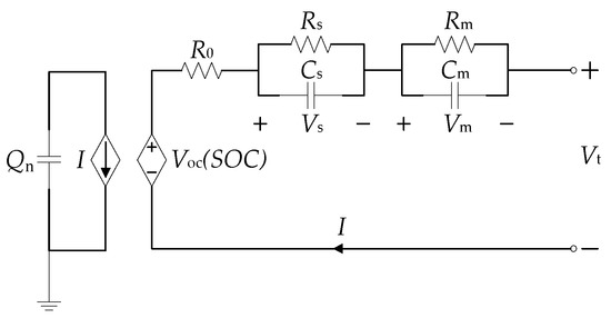
Figure 1.
Second-order RC equivalent circuit model.
The SRCECM consists of the following:
- (1)
- The capacitor Qn represents the total stored energy in the battery. The controlled voltage source Voc(SOC) is used to establish the nonlinear relationship between the SOC and the OCV, as shown in Figure 2.
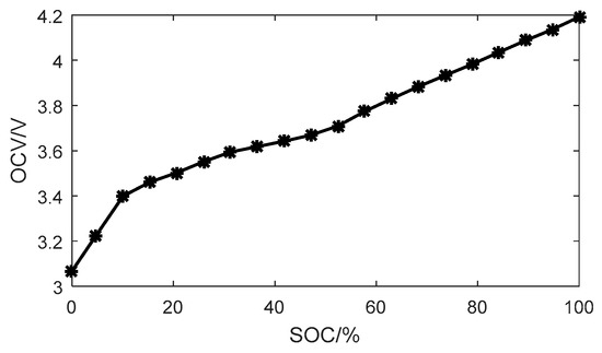 Figure 2. Open circuit voltage (OCV)–state of charge (SOC) curve.
 - (2)
- R0 is the ohmic resistance, which indicates the internal energy loss of the battery during the charge/discharge process.
- (3)
- The parallel network RsCs represents the concentration polarization which reflects the effect of the diffusion of the reactant and product in the electrochemical reaction. RmCm represents the electrochemical polarization, which describes the structure of the double layer of the electrode/solution interface.
In addition, due to extremely low self-discharge rate of a Li-ion battery, the self-discharge resistance is ignored in the model.
Vt and I represent the terminal voltage and current, respectively. I > 0 represents discharge and I < 0 represents charge. According to Kirchhoff’s law, Vt can be expressed as
The differential expressions for the SOC, the concentration polarization voltage Vs, and the electrochemical polarization voltage Vm are
During a small range of the SOC indicated by the asterisks in Figure 2, the nonlinear relationship between the OCV and SOC can be considered linear [19]. Therefore, the OCV is expressed as a linear function of the SOC by using the piecewise linearization method:
where k0 and k1 are the different constants for different SOC ranges.
For the fast sampling frequency in SOC estimation, the current change rate can be ignored; namely, dI/dt = 0. We substitute Equations (2)–(5) into the derivative of Equation (1) and rearrange the differential equation:
where the term is added into Equation (6), which represents the differential error, the modeling error, and uncertain disturbances such as measurement noise.
Solving I in Equation (1) and substituting it into Equation (2), as well as rearranging Equations (3) and (4), results in the state–space equations of the SRCECM as follows:
where b1 = k0/Qn + R0/(RsCs) + 1/Cs + R0/(RmCm) + 1/Cm; b2 = 1/Cs; b3 = 1/Cm; a1 = 1/(RsCs) + 1/(RmCm); a2 = 1/(R0Qn); a3 = 1/(RsCs); and a4 = 1/(RmCm).
The current and terminal voltage of the battery can be measured, and it is easy to represent the system of the SRCECM as:
where x = [Vt SOC Vs Vm]T is the state vector, and u(t) = I and y(t) = Vt are the input and output of the system, respectively. The matrices A, B, and C are defined as
where is the constant matrix corresponding to the SOC range.
The main objective of this paper is to design an observer which is able to estimate the battery SOC based on the model given by Equation (7). The prerequisite of the successful application of the observer is that the system given by Equation (8) is observable. The observability proof is as follows: the observability matrix is
The full rank of O(M) is verified by using the model parameters (derived from Section 2.2); thus, the system of the SRCECM is observable and the state variables can be estimated by the observer.
2.2. Model Parameter Identification
The experimental platform shown in Figure 3 was built to identify the model parameters and estimate the SOC. The Li-ion battery used in the experiment comprises a graphite cathode and a ternary composite anode of nickel, cobalt, and aluminum. It has a nominal capacity of 2.5 Ah and a nominal voltage of 3.6 V. The dimensions of the Li-ion battery are 18 mm diameter and 65 mm height. This kind of battery is commonly referred to as being of the “18650” format. The battery test system is used to charge or discharge the battery, which has a built-in current integrator that can be used to calculate the SOC reference. Its measurement ranges are 0~5 V and 0~5 A, and the measurement accuracy is ±5 mV/±5 mA. The upper software controls the charging or discharging mode and records the voltage and current data. The sampling interval was 10 s, and the experiment was carried out at room temperature.
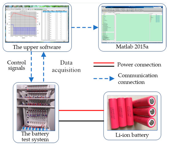
Figure 3.
The experimental platform.
Model parameter identification is used to make the model output as close to the battery output as possible utilizing the input and output of the battery with the aid of some mathematical algorithms. Currently, the off-line identification method is more widely applied, since on-line identification is sensitive to the initial values of coefficients and has stability problems due to the cross interference between the model parameters and SOC [30]. A more robust off-line identification method is to fit rest periods of experimental data with exponential functions; therefore, based on the above principle, the pulse current discharge profile as an off-line approach was applied to identify the model parameters. As shown in Figure 4a, the pulse current profile consists of many sequences of discharge and rest. Initially, the battery was fully charged (SOC = 100%) and rested for one hour to return to the equilibrium state. Then, the battery was discharged by 0.5 A, corresponding to a 0.2 C discharge ratio for 15 min. After the discharge process, the battery was rested for 1 h to allow the terminal voltage to reach the OCV. Each pulse current discharged approximately 5% of the actual capacity of the battery, which is equivalent to about 5% of the SOC. The sequence of discharge and rest was iterated until the terminal voltage was less than the cut-off voltage of 2.5 V, meaning that the battery was fully discharged (SOC = 0%). The last discharge data was abandoned because of the lack of the last resting period data. It can be seen that there were 18 transient voltage responses generated to determine 18 groups of model parameters for 18 different SOCs. Incidentally, the nonlinear relationship between the OCV and the SOC was obtained, as shown in Figure 2. The specific parameter identification process is as follows.
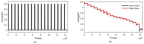
Figure 4.
The 0.2 C pulse current discharge profile: (a) the current; (b) the voltage.
During each rest period of the battery, the terminal voltage response can be expressed using Equation (11):
where and are the time constants of concentration polarization and electrochemical polarization, respectively. As an example, the seventh terminal voltage (actual value) response is indicated by a red square in Figure 4b where the framed section is magnified in Figure 5. The terminal voltage response profile was fitted based on Equation (11) with the Cftool Matlab fitting tool; thereby, the parameters of , , , and were solved.
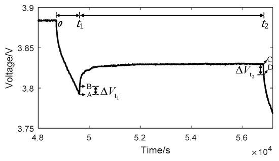
Figure 5.
Transient voltage response.
At the time of , the battery finishes the discharge of a certain sequence, and the polarization voltages are
, , , and can be derived as follows:
In addition, the ohmic resistance is given by
The identified model parameters for the different SOCs are listed in Table 1 with the curve fitting errors represented by root mean square errors (RMSE). The SRCECM has a very small deviation in the fitting profile. For the last rest sequence, the identified parameters cause the largest model error because the polarization effect of the battery is the most serious. The fitted voltage of the model is compared with the actual voltage in Figure 4b and Figure 6, showing the voltage error of the model. The voltage error is quite small in the range SOC [0.1 1]. The largest error also exists around the cut-off voltage region. The model RMSE is 0.0037. To test the model’s flexibility, another larger constant current (0.8 C) profile was applied to both the battery and the established model. The model voltage compared with the actual voltage of the battery is shown in Figure 7a, in which the model’s voltage error has similar characteristics as in Figure 4b. The voltage error is shown in Figure 7b. The discharge end area also has large modeling error while the other error is quite small. The model RMSE is 0.0156.

Table 1.
The identified model parameters.
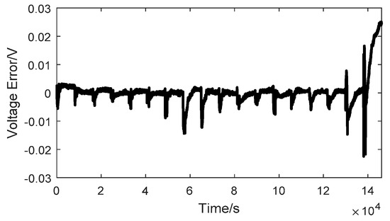
Figure 6.
The voltage error of the model.
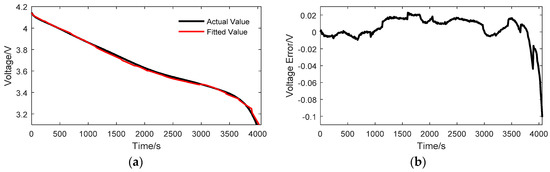
Figure 7.
The 0.8 C constant current discharge profile: (a) the voltage; (b) the voltage error.
3. The Design of the Super-Twisting Sliding Mode Observer for SOC Estimation
3.1. Super-Twisting Sliding Mode Observer
In this paper, the ST algorithm was applied to design a sliding mode observer for the SOC estimation of the battery. Considering the following system of the SRCECM, and defining as the sliding mode variable and , the proposed SMO is formulated as
where , , , and are the estimated states; and , , and are the coefficients of the proposed SMO. () is the ST algorithm
and and are the gains of the ST algorithm. sign(σ) is the symbol function defined as follows:
The ST algorithm is composed of two parts: The first part is a continuous function (), which can be regarded as a proportional term. While the system error appears, it has quick response speed to reduce the error for the following reasons: when , is large, which increases the proportional gain . When , the STSMO achieves large gain with small bias for . The second part is the time integral , which helps to eliminate the system error for the observed system.
We define other observation errors as
Subtracting Equation (15) from Equation (7), the state estimation error system is given as follows:
3.2. Stability Proof
Assumption 1.
The systems of the equivalent circuit model (Equation (7)) and the observer system (Equation (15)) are bounded input, bounded state (BIBS) since this is a physical system and the battery current and voltage are both bounded according to the battery operation conditions, which are controlled by the battery test system.
Theorem 1.
The termrepresents the error system uncertainties, and is assumed to satisfy the following condition:
where the boundsandare positive constants which can be determined by the largest model error from experiments or experts’ experience. Therefore, the state estimation error system (Equations (19)–(22)) is asymptotically stable.
Proof of Theorem 1.
The proof is divided into two parts. First, Equation (19) is proven to converge to zero in finite time. Second, the resulting reduced-order dynamics of Equations (20)–(22) are proven to be exponentially stable [28].
The system given by Equation (19) can be rewritten as
where . Equation (24) can be understood as the sliding mode dynamic property along the system trajectory. is the sliding mode variable and the relative order of the system given by Equation (19) is 1. Therefore, the ST algorithm can make in finite time with and , while can be made for the CSM.
Based on Assumption 1, the state does not go to infinity in finite time for the reason that the input I is bounded. Moreover, is bounded and all the states of the observer are also bounded for a finite time. Consequently, the observation error is also bounded. It follows from Equations (20)–(22) that and are bounded. So, it can be assumed that where is an unknown constant.
Define . Due to and , the characteristic polynomial is and M is a Hurwitz matrix. Thus, there must exist a positive-definite symmetric matrix P which satisfies the Lyapunov equation for a positive-definite symmetric matrix Q:
Then, the following Lyapunov function V is introduced:
which can be rewritten in quadratic form
where
Note that is differentiable everywhere except and is radially unbounded. The system state does not stay at until the system converges to the origin . With (), the derivative of is
Taking the derivative of Equation (27) along the trajectory,
where
Because is a quadratic positive-definite function, there exists
where (P) and (P) are the minimum eigenvalue and maximum eigenvalue of the matrix P, respectively; is a 2-norm of Euclidean space ; and . It can be further obtained as follows:
Therefore,
Using Equation (32) and the fact that
it follows that
By the comparison principle, it follows that and therefore converge to zero in finite time. Thus, Theorem 1 is proven.
It follows from Theorem 1 that when the sliding motion takes place, . Thus, the equivalent injection () can be directly obtained from Equation (19):
Substituting Equation (37) into the error system given by Equations (20)–(22) and denoting , the following reduced-order system is obtained:
where
Consider a candidate Lyapunov function for the system in Equation (38):
where there exists a symmetric positive-definite matrix which satisfies and is an identity matrix.
The time derivative of along the trajectories of the system in Equation (38) is presented as
According to Equation (41), is always negative. Therefore, the resulting reduced-order dynamics in Equation (38) are proven to be exponentially stable. ☐
3.3. Coefficients of the STSMO
According to the Schur lemma, matrices P and Q will be positive when satisfying the condition and large enough, as for the example and where is explained in Equation (23), and the system errors will then converge to zero in finite time [31]. In order to make the ST algorithm convenient for application, the coefficients and are further discussed in [32,33]. Reference [33] gives the following sufficient conditions:
where L is the Lipschitz’s constant of the sliding mode variable, L > 0. Condition (42) results from a very crude estimation. In practice, one way to choose and is to take
with properly chosen values of and . In particular, both and are valid choices.
The other coefficients , , and of the STSMO can be determined by experiments after many rounds of debugging.
4. Experimental Results for SOC Estimation
The configuration of the STSMO for the SOC estimation is illustrated in Figure 8. The upper software executes the discharge command and the Li-ion battery is discharged according to the established current mode. The actual current and voltage of the battery are sampled constantly every 10 s and fed into the model to obtain the model parameters. Then, the STSMO updates the SOC based on the observation error utilizing all the parameters and sampling data.
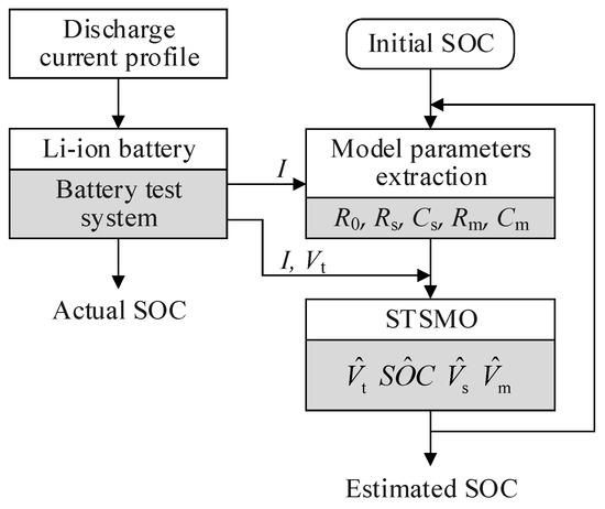
Figure 8.
Configuration of the super-twisting sliding mode observer (STSMO) system.
The coefficients of STSMO were selected as , , , , and . To further illustrate the advantages of the proposed observer, the SOC estimation results are firstly compared with the CSMO to verify the necessity of HOSM application. Then the superiority of the STSMO is proven by comparing with the well-established algorithm, namely, the AEKF proposed in [12]. The initial values of the process noise variance matrix Rk, the measurement noise variance matrix Qk, and the system covariance matrix Pk are , , and , where I is an identity matrix. In addition, three different discharge profiles are utilized to evaluate the SOC estimation effect of the STSMO. The evaluation indices include SOC estimation accuracy, computation time, convergence speed, and robustness against noise disturbances. Besides the 0.5 C pulse current discharge (PCD) profile, other two discharge profiles were 0.2 C constant current discharge (CCD), and dynamic stress test (DST) discharge (shown in Figure 9). The DST discharge profile is a simplified version of the United States Advanced battery Consortium (USABC) Electric Vehicle Battery Test Procedures Manual. Before loading each discharge current, the battery is fully charged (the initial SOC = 100%) and rested for 1 h to reach the steady state.
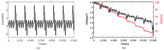
Figure 9.
Dynamic stress test (DST) discharge profile: (a) the current; (b) the terminal voltage and the SOC.
4.1. Comparison between STSMO and CSMO
The CSMO is designed as
where is the switching gain and was chosen. As an example, the results of the 0.2 C CCD profile are shown in Figure 10. It can be found the SOC estimation of the CSMO has high track accuracy and proper chattering. Unfortunately, when the initial SOC deviates from its true value, e.g., 30% and 60% error, the SOC estimation errors are reduced to 5% after 930 s and 3530 s, respectively, and the convergence speed is very slow, as shown in Figure 11. In Figure 12, with relatively large gain, the CSMO achieves faster SOC estimation convergence, but significant chattering is generated on the SOC estimation results due to its discontinuous switching property. The error of Figure 12 shows that the chattering width is approximate 0.5%. As shown in Figure 13, the STSMO can eliminate the chattering significantly with reasonable convergence speed. This is due to the fact that the STSMO transfers the chattering into the HOSM surface and thereby attenuates the chattering. Therefore, compared with the CSMO, the STSMO demonstrates its superiority in terms of chattering for SOC estimation.
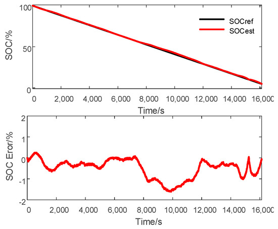
Figure 10.
Conventional sliding mode observer (CSMO)-based SOC estimation.
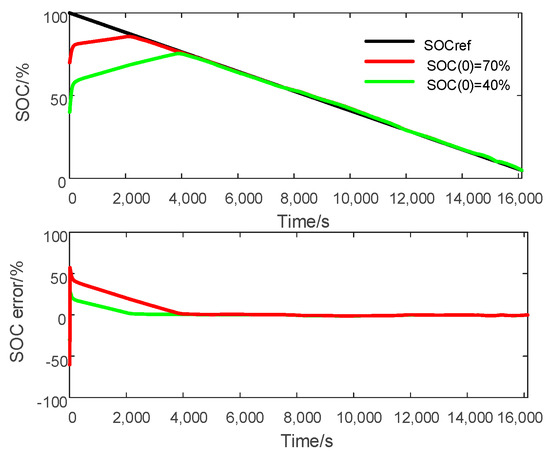
Figure 11.
CSMO-based SOC estimation at different initial SOCs.
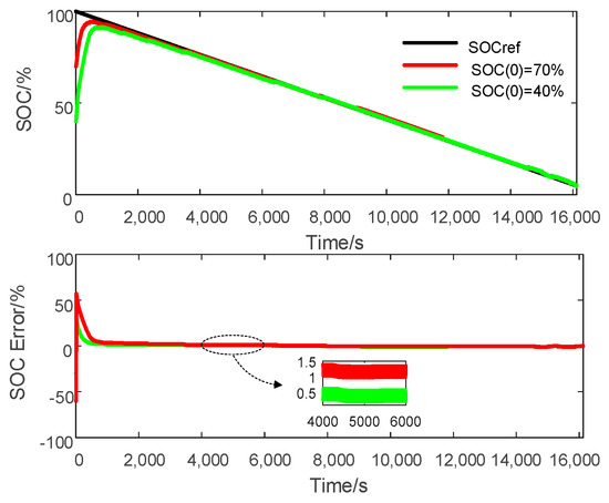
Figure 12.
CSMO-based SOC estimation at different initial SOCs with large switching gain.
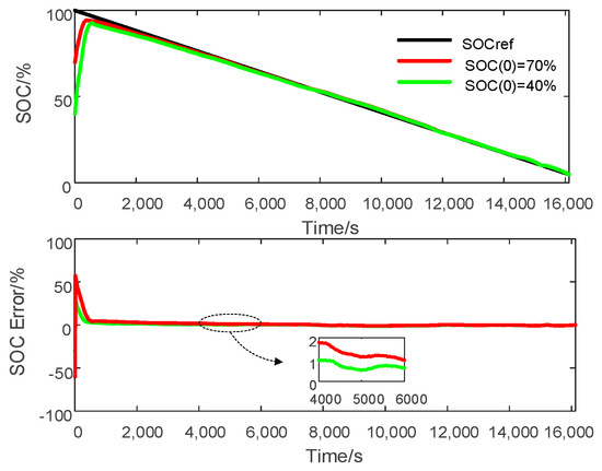
Figure 13.
STSMO-based SOC estimation at different initial SOCs
4.2. Comparison between STSMO and AEKF
• SOC Estimation with True Initial SOC Value and No Noise
Figure 14, Figure 15 and Figure 16 show the comparison of SOC estimation results between the AEKF and STSMO under three different discharge profiles. It can be found that both methods can track the SOC reference accurately. However, according to the error in Figure 14, Figure 15 and Figure 16, the SOC estimation errors of the STSMO are closer to zeros while the errors of the AEKF are just bounded in by about ±5%. To quantificationally illustrate the improved accuracy of the STSMO-based SOC estimation, Table 2 lists the RMSE of the SOC estimation at different discharge profiles. It can be seen that the RMSE of the STSMO is always smaller than that of AEKF for the three different discharge profiles.
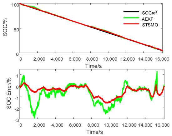
Figure 14.
SOC estimation for 0.2 C constant current discharge (CCD) profile. AEKF: adaptive extended Kalman filter.
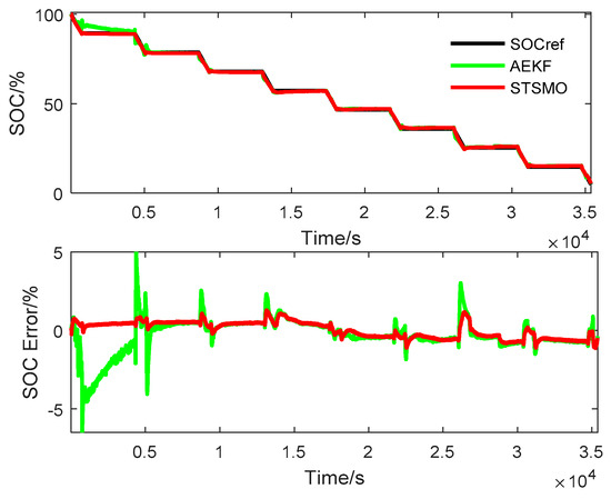
Figure 15.
SOC estimation for 0.5 C pulse current discharge (PCD) profile.
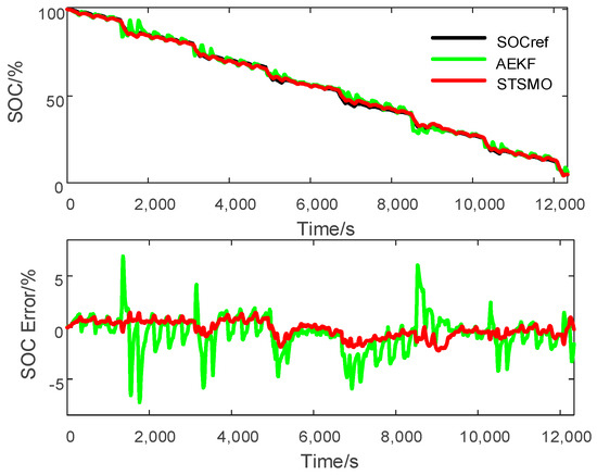
Figure 16.
CSMO-based SOC estimation at different initial SOCs with large switching gain.
Table 2.
RSME of SOC estimation error.
In addition, Table 3 shows the computation time for SOC estimation by the two methods at different discharge profiles. The computation time was obtained by the tic/toc program of MATLAB (2015a, MathWorks, Natick, MA, USA). The computer’s CPU was an i5-4590 and the basic frequency was 3.3 GHz. After running the program many times, the maximum value of the time was chosen and presented in Table 3. It is obvious that the computation time of the STSMO is less than that of the AEKF. The reason for this is that the STSMO makes a direct state correction while the AEKF executes a priori estimation and then corrects for the system states. Therefore, the STSMO has shown outstanding capability to track the SOC reference accurately.
Table 3.
Computation time for SOC estimation of two methods (unit: s).
• SOC Estimation with Different Initial SOCs
A fast convergence speed helps to improve the capability to track the SOC reference at any initial SOC (e.g., 70% and 40%). Figure 17 presents the SOC convergence process of the STSMO and AEKF at different initial SOCs for the DST discharge profile. Table 3 gives the corresponding convergence time, which is the time that the SOC error is reduced to 5%. According to Figure 17 and Table 4, it is clear that the convergence speed of the STSMO-based SOC estimation is faster than that of the AEKF-based SOC estimation, and the SOC convergence time of the AEKF is more than 3 times that of the STSMO. Therefore, compared with the AEKF, the STSMO has faster convergence speed at certain initial SOC deviations.
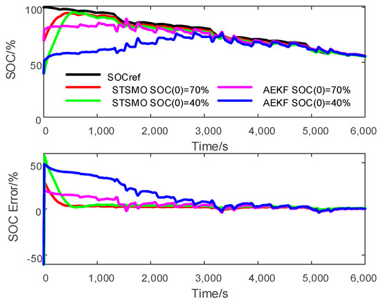
Figure 17.
SOC convergence process for the DST discharge profile at different initial SOCs.
Table 4.
SOC convergence time at different initial SOCs.
• SOC Estimation with Added Noise Disturbances
In an on-line system, it is difficult to obtain accurate voltage/current values due to sensor precision and electromagnetic interference. To evaluate the robustness of the STSMO, random normally distributed noise was added to the measurement signals, i.e., voltage and current. The mean value of the noise was zero and the standard deviations (SD) SD = 0.01 and SD = 0.03 were studied. The SOC estimation results based on the STSMO and AEKF with two kinds of different noises are shown in Figure 18, and the error range is summarized in Table 5.
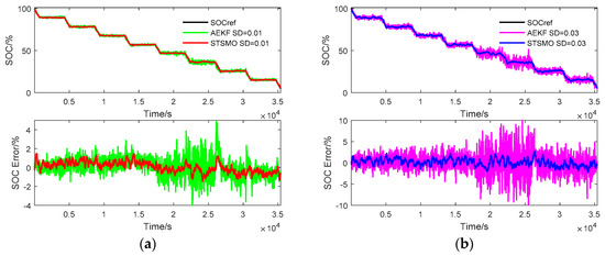
Figure 18.
SOC estimation for 0.5 C PCD profile with added noise disturbances. (a) SD = 0.01 V; (b) SD = 0.03 V.
Table 5.
The SOC estimation error range with different amplitude SDs.
Obviously, the maximum errors of both the STSMO and AEKF increase with the increase of the SD, but the values of the STSMO increase far less than those of the AEKF. The STSMO can also track the SOC reference with small error, bounded by about ±2%. In addition, it can be found that the maximum of the AEKF becomes unexpectedly smaller when the SD is from 0 to 0.01. The reason for this is that it hardly works for relatively accurate measurement signals such as laboratory data, although AEKF has strong robustness against low levels of noise. On the whole, the STSMO has stronger robustness against noise disturbance.
5. Conclusions
On the basis of the established SRCECM, the STSMO was presented to estimate battery SOC. Lyapunov stability analysis was utilized to prove the convergence of the error system of the observer. Three different discharge profiles—PCD, CCD, and DST—were carried out to evaluate the performance of the SOC estimation. The experimental comparisons with the CSMO showed that the STSMO can solve the chattering problem and improve the convergence speed, and the superiority of the HOSM application is thereby verified. Furthermore, the comparisons with the AEKF indicate that the STSMO has better performance in improving the estimation accuracy, reducing the computation time, accelerating the convergence speed and enhancing the robustness against noise disturbances. The proposed STSMO is suitable for on-line SOC estimation.
Author Contributions
All authors have worked on this manuscript together and all authors have read and approved this manuscript.
Acknowledgments
This work was supported by the Shaanxi Science and Technology Co-ordination Innovation Project, China under Grant 2015KG090203 and the Xi’an Key Cultivation Project of the Transformation of Sci-Tech Achievements under Grant N2017KE0100.
Conflicts of Interest
The authors declare no conflict of interest.
References
- Hannan, M.; Lipu, M.; Hussain, A.; Mohamed, A. A review of lithium-ion battery state of charge estimation and management system in electric vehicle applications: Challenges and recommendations. Renew. Sustain. Energy Rev. 2017, 78, 834–854. [Google Scholar] [CrossRef]
- Jaguemont, J.; Boulon, L.; Dubé, Y. A comprehensive review of lithium-ion batteries used in hybrid and electric vehicles at cold temperatures. Appl. Energy 2016, 164, 99–114. [Google Scholar] [CrossRef]
- Xing, Y.; He, W.; Pecht, M.; Tsui, K.L. State of charge estimation of lithium-ion batteries using the open-circuit voltage at various ambient temperatures. Appl. Energy 2014, 113, 106–115. [Google Scholar] [CrossRef]
- Duong, V.; Bastawrous, H.A.; Lim, K.; See, K.W.; Zhang, P.; Dou, S.X. Online state of charge and model parameters estimation of the LiFePO 4 battery in electric vehicles using multiple adaptive forgetting factors recursive least-squares. J. Power Sources 2015, 296, 215–224. [Google Scholar] [CrossRef]
- Chen, J.; Ouyang, Q.; Xu, C.; Su, H. Neural Network-Based State of Charge Observer Design for Lithium-Ion Batteries. IEEE Trans. Control Syst. Technol. 2018, 26, 313–320. [Google Scholar] [CrossRef]
- Chen, Z.; Mi, C.C.; Fu, Y.; Jun, X.; Gong, X. Online battery state of health estimation based on Genetic Algorithm for electric and hybrid vehicle applications. J. Power Sources 2013, 240, 184–192. [Google Scholar] [CrossRef]
- Antón, J.; Nieto, P.; Viejo, C.B.; Vilan, J.A.V. Support Vector Machines Used to Estimate the Battery State of Charge. IEEE Trans. Power Electron. 2013, 28, 5919–5926. [Google Scholar] [CrossRef]
- Waag, W.; Fleischer, C.; Sauer, D.U. Critical review of the methods for monitoring of lithium-ion batteries in electric and hybrid vehicles. J. Power Sources 2014, 258, 321–339. [Google Scholar] [CrossRef]
- Yuan, S.; Wu, H.; Yin, C. State of Charge Estimation Using the Extended Kalman Filter for Battery Management Systems Based on the ARX Battery Model. Energies 2013, 6, 444–470. [Google Scholar] [CrossRef]
- Wang, Y.; Liu, C.; Pan, R.; Chen, Z. Modeling and state-of-charge prediction of lithium-ion battery and ultracapacitor hybrids with a co-estimator. Energy 2017, 121, 739–750. [Google Scholar] [CrossRef]
- Li, D.; Ouyang, J.; Li, H.; Wan, J. State of charge estimation for LiMn2O4, power battery based on strong tracking sigma point Kalman filter. J. Power Sources 2015, 279, 439–449. [Google Scholar] [CrossRef]
- Xiong, R.; He, H.; Sun, F.; Zhao, K. Evaluation on State of Charge Estimation of Batteries with Adaptive Extended Kalman Filter by Experiment Approach. IEEE Trans. Veh. Technol. 2013, 62, 108–117. [Google Scholar] [CrossRef]
- Xiong, R.; Gong, X.; Mi, C.C.; Sun, F.C. A robust state-of-charge estimator for multiple types of lithium-ion batteries using adaptive extended Kalman filter. J. Power Sources 2013, 243, 805–816. [Google Scholar] [CrossRef]
- Yu, Q.; Xiong, R.; Lin, C.; Shen, W.; Deng, J. Lithium-Ion Battery Parameters and State-of-Charge Joint Estimation Based on H-Infinity and Unscented Kalman Filters. IEEE Trans. Veh. Technol. 2017, 66, 8693–8701. [Google Scholar] [CrossRef]
- He, Z.; Chen, D.; Pan, C.; Chen, L.; Wang, S. State of charge estimation of power Li-ion batteries using a hybrid estimation algorithm based on UKF. Electrochim. Acta 2016, 211, 101–109. [Google Scholar]
- Wang, Y.; Zhang, C.; Chen, Z. A method for joint estimation of state-of-charge and available energy of LiFePO4 batteries. Appl. Energy 2014, 135, 81–87. [Google Scholar] [CrossRef]
- Chen, C.; Xiong, R.; Shen, W. A lithium-ion battery-in-the-loop approach to test and validate multi-scale dual H infinity filters for state of charge and capacity estimation. IEEE Trans. Power Electron. 2018, 33, 332–342. [Google Scholar] [CrossRef]
- Hu, X.; Sun, F.; Zou, Y. Estimation of State of Charge of a Lithium-Ion Battery Pack for Electric Vehicles Using an Adaptive Luenberger Observer. Energies 2010, 3, 1586–1603. [Google Scholar] [CrossRef]
- Xu, J.; Mi, C.C.; Cao, B.; Deng, J.; Chen, Z.; Li, S. The State of Charge Estimation of Lithium-Ion Batteries Based on a Proportional-Integral Observer. IEEE Trans. Veh. Technol. 2014, 63, 1614–1621. [Google Scholar]
- Xia, B.; Chen, C.; Tian, Y.; Sun, W.; Xu, Z.; Zheng, W. A novel method for state of charge estimation of lithium-ion batteries using a nonlinear observer. J. Power Sources 2014, 270, 359–366. [Google Scholar] [CrossRef]
- Li, W.; Liang, L.; Liu, W.; Wu, X. State of Charge Estimation of Lithium-Ion Batteries Using a Discrete-Time Nonlinear Observer. IEEE Trans. Ind. Electron. 2017, 64, 8557–8565. [Google Scholar] [CrossRef]
- Kim, I. Nonlinear State of Charge Estimator for Hybrid Electric Vehicle Battery. IEEE Trans. Power Electron. 2008, 23, 2027–2034. [Google Scholar]
- Kim, I. A Technique for Estimating the State of Health of Lithium Batteries through a Dual-Sliding-Mode Observer. IEEE Trans. Power Electron. 2010, 25, 1013–1022. [Google Scholar]
- Huangfu, Y.; Zhuo, S.; Rathore, A.K.; Breaz, E.; Nahid-Mobarakeh, B.; Gao, F. Super-Twisting Differentiator-Based High Order Sliding Mode Voltage Control Design for DC-DC Buck Converters. Energies 2016, 9, 494. [Google Scholar] [CrossRef]
- Moreno, J.A.; Osorio, M. A Lyapunov approach to second-order sliding mode controllers and observers. In Proceedings of the 47th IEEE Conference on Decision and Control, Cancun, Mexico, 9–11 December 2008; pp. 2856–2861. [Google Scholar]
- Chen, X.; Shen, W.; Cao, Z.; Kapoor, A. A novel approach for state of charge estimation based on adaptive switching gain sliding mode observer in electric vehicles. J. Power Sources 2014, 246, 667–678. [Google Scholar] [CrossRef]
- Du, J.; Liu, Z.; Wang, Y.; Wen, C. An adaptive sliding mode observer for lithium-ion battery state of charge and state of health estimation in electric vehicles. Control Eng. Pract. 2016, 54, 81–90. [Google Scholar] [CrossRef]
- Liu, J.; Laghrouche, S.; Wack, M. Observer-based higher order sliding mode control of power factor in three-phase AC/DC converter for hybrid electric vehicle applications. Int. J. Control 2014, 87, 1117–1130. [Google Scholar] [CrossRef]
- Liu, J.; Laghrouche, S.; Harmouche, M.; Wack, M. Adaptive-gain second-order sliding mode observer design for switching power converters. Control Eng. Pract. 2014, 30, 124–131. [Google Scholar] [CrossRef]
- Wei, Z.; Lim, T.M.; Skyllas-Kazacos, M.; Wai, N.; Tseng, K.J. Online state of charge and model parameter co-estimation based on a novel multi-timescale estimator for vanadium redox flow battery. Appl. Energy 2016, 172, 169–179. [Google Scholar] [CrossRef]
- Dávila, A.; Moreno, J.A.; Fridman, L. Optimal Lyapunov function selection for reaching time estimation of Super Twisting algorithm. In Proceedings of the 48th IEEE Conference on Decision and Control and 28th Chinese Control Conference, Shanghai, China, 16–18 December 2009; pp. 8405–8410. [Google Scholar]
- Davila, J.; Fridman, L.; Levant, A. Second-order sliding-mode observer for mechanical systems. IEEE Trans. Autom. Control 2005, 50, 1785–1789. [Google Scholar] [CrossRef]
- Levant, A. Robust Exact Differentiation via Sliding Mode Technique; Pergamon Press: Great Britain, UK, 1998; pp. 379–384. [Google Scholar]
© 2018 by the authors. Licensee MDPI, Basel, Switzerland. This article is an open access article distributed under the terms and conditions of the Creative Commons Attribution (CC BY) license (http://creativecommons.org/licenses/by/4.0/).