Electric Vehicle Fast-Charging Station Unified Modeling and Stability Analysis in the dq Frame

Abstract

The electric vehicle fast-charging station is an important guarantee for the popularity of electric vehicle. As the fast-charging piles are voltage source converters, stability issues will occur in the grid-connected fast-charging station. Since the dynamic input admittance of the fast-charging pile and the dynamic output impedance play an important role in the interaction system stability, the station and grid interaction system is regarded as load-side and source-side sub-systems to build the dynamic impedance model. The dynamic input admittance in matrix form is derived from the fast-charging pile current control loop considering the influence of the LC filter. Similarly, the dynamic output impedance can be obtained similarly by considering the regional power grid capacity, transformer capacity, and feed line length. On this basis, a modified forbidden region-based stability criterion is used for the fast-charging station stability analysis. The frequency-domain case studies and time-domain simulations are presented next to show the influence of factors from both the power grid side and fast-charging pile side. The simulation results validated the effectiveness of the dq frame impedance model and the stability analysis method.

1. Introduction

In recent years air pollution and haze have caused health issues around all the world. It is now becoming a more and more serious social problem that calls for less fossil fuels and more renewable energy. As a large consumer of fossil fuels, the transportation sector has emitted about 25% of the greenhouse gases produced by energy-related sectors, so the automobile’s energy structure mode change is imperative [1]. The demand of green transportation is growing rapidly due to these problems, and electric vehicles (EVs) are widely regarded as a proper solution for this problem. Some countries and regions, such as China and Europe, will start researching the exit schedule of traditional-fuel vehicles [2,3]. This will contribute to the enhancement of the development and deployment of electric vehicles and lead to more and more EVs entering the market [4].

A large number of EVs require a large charging infrastructure to supply the electricity need. Generally, the EV power battery capacity varies from about 20 kWh to more than 100 kWh. According to the SAE J1772 standard [5], there are three charging standards for EVs that have been developed [6,7,8]:

Level 1: The charging equipment uses single-phase AC power of 120 V voltage and 12 to 16 A current. It takes more than 10 h for a level 1 charger to charge a 20 kWh EV battery from 0% state of charge (SOC) to 100% SOC.

Level 2: The charging equipment uses 208–240 V single-phase AC power to provide up to 19.2 kW of charging power, needing at least 1 h for charging a 20 kWh EV battery to full SOC.

Level 3: This also known as fast-charging, the voltage used in this system is rated to 380 V in the AC side, 600 V in the DC side, and the maximum current is up to 400 A to provide a maximum 240 kW charge power. A 100 kWh EV battery can be fully charged within less than half an hour.

The common slow-charging piles are usually located in residential and office or shopping mall building parking lots, which cannot satisfy the sudden charging requirement due to the limitations of time and space. As a supplement to the slow charging, the EV fast-charging station is a necessary supplement and vital components for public acceptance of electric vehicles because it can greatly improve the ease of use for the EV owners. It makes the electricity energy refill as easy as refueling gasoline.

The EV fast-charging station generally consists of a distribution transformer and multiple fast-charging piles that are three-phase AC–DC voltage source converters (VSC) to generate the DC voltage for the EV battery. Since the fast-charging piles can provide a maximum charging power more than 200 kW, suppose that a EV fast-charging station contains 10 charging piles, when 10 are EVs charging simultaneously, the load can be up to 2000 kW, which is about the same as a residential or office building. Large numbers of EVs connecting to the urban power grid through EV fast-charging stations will change the dynamic characteristics of the power system since the fast-charging piles are controlled power electronic devices. EV fast-charging stations, together with the VSC-connected renewable generators, e.g., wind power and solar power, lead the power grid to power electronic features and make the AC grid relatively weak [9,10]. Under such a situation, the interaction between the VSCs and the AC power grid will lead to complex oscillation problems. Such oscillation instability issues appeared in railway traction and supply systems where pantograph rising has been reported, a swing of the peak value of the grid side voltage appears on the sinusoidal wave as a low-frequency oscillation (LFO) [11]. In Texas and the Hebei province of China, interaction between wind power plants and the power grid lead to a sub-synchronous oscillation that will influence the stability of the power plant [12,13]. Sub-synchronous oscillation between the wind power plants even led to tripping of power plant units in Xinjiang. These instability issues are known to be caused by the power electronic interface loads and generators, such as electric vehicles, wind power plants, solar power plants, and electrified railway interaction with the power grid and interaction between these loads and generation.

Compared with the traditional LFO, the mechanism of interaction among VSCs and the AC grid is more complex and has not been fully understood. These kinds of power electronic interfaced oscillation and instability issues are generally analyzed from the viewpoint of small disturbances by the method of eigenvalues based on the state space model [14] and the impedance method based on frequency theory [15,16,17]. The eigenvalue method is difficult to apply in the large-scale system with the high penetration of power electronic interfaced loads and generators due to its requirement of detailed models and parameters of the converters and the power system. Compared with the eigenvalue method, the impedance-based method regards the interaction system as two sub-systems, comprised of the load side converter and the source side AC grid at the point of common coupling (PCC). Only the output and input characteristics at the PCC of both sub-systems are concerned in this method to analyze the stability of the interaction system. In recent years the impedance method has been adopted in the stability analysis for grid-connected VSCs [18,19]. Jian has proposed an impedance-based method in [19] by using the Nyquist criterion to analyze the stability of grid connected inverters. However, this method is developed for the single input and single output (SISO) system, and it is not suitable for stability analysis of the fast-charging station.

Generally, the three-phase AC–DC fast-charging piles are controlled in the dq frame. Thus, this paper builds the mathematical model of the three-phase fast-charging pile under the dq frame by using the transformation relationship between stationary frame and rotate frame. The fast-charging pile is considered as a multi-input multi-output (MIMO) system under the dq frame. In this mathematical model, the input variable and output variable are both two-dimensional vectors, the output impedance and input admittance are also a two-dimensional square matrix. The stability of the MIMO system can be analyzed based on the impedance-based method. That is based on the output impedance matrix of the grid side and the input admittance matrix of the fast-charging pile side.

In the dq frame dynamic model, the traditional impedance-based method cannot be used for stability analysis. For the MIMO system with the asymmetric impedance/admittance matrix, the generalized Nyquist criterion proposed by MacFarlane and Postlethwaite is widely used for stability assessment [20]. Except the generalized Nyquist criterion, some other methods are proposed for the AC cascade system, such as singular value criterion [21,22], D channel criterion [23,24,25], and norm criterion [26]. Compared with traditional methods, such as the Bode diagram, Nyquist criterion, dominate pole, etc., these methods are simpler in calculation. Singular value criterion and norm criterion have some conservatism in stability analysis, and the D channel criterion is obtained from experimental results of high power factor cascade systems, and it is not a sufficient condition, theoretically. The application of D channel criterion is limited since its validity in other AC cascade system cannot be guaranteed. A forbidden region-based stability analysis method in the dq frame that can be classified as a D channel criterion is proposed in [27]. Since the high power factor condition cannot be met when instability occurs, the D channel criterion cannot be used for the EV fast-charging station stability analysis. Based on these methods, a novel stability criterion based on a different forbidden region from [28] is adopted for stability analysis of an EV fast-charging station in this paper.

This paper develops the dynamic impedance model of the EV fast-charging system in the dq frame at the point of common coupling, and stability of the fast-charging station is analyzed by using the novel forbidden region-based criterion. The rest of the paper is organized as follows: the detailed description of the EV fast-charging system, including the structure, connection, and control diagram is proposed in Section 2. Then the dynamic model of the EV fast-charging station and grid interaction system is presented in Section 3. In this part, the control system topology of the three-phase voltage source converter is presented, the dynamic model includes the matrix form input admittance of the fast-charging pile and the matrix output impedance of the AC grid side. The input admittance of the fast-charging pile is derived from the current control loop by using the frame transformation, and the dynamic model of the grid side is obtained through the output impedance of the grid system, including the power source, transformer, and distribution line, is presented. Frequency domain stability analysis is presented in Section 4. Furthermore, the time domain simulations are presented in Section 5 to validate the model proposed in this paper.

2. EV Fast-Charging Station Interaction System Dynamic Model

2.1. EV Fast-Charging System Description

Generally, the EV fast-charging station is supplied by the power grid through a distribution transformer via overhead lines or underground cables. The single-line electric diagram of the EV fast-charging station connected to the power grid through a substation transformer is shown in Figure 1. The source represents the power grid and one transformer is included in the substation, the AC bus represents the high voltage and low voltage of the substation, respectively. The fast-charging pile is the connection between the EV and the grid as Figure 1 shows.

2.2. Control System Introduction of the Fast-Charging Pile

The EV fast-charging pile in in the station is a three-phase AC/DC voltage source converter. The electrical tropology of the fast-charging pile is shown in Figure 2.

As mentioned above, the fast-charging pile is a PWM-controlled three-phase AC/DC voltage source converter. The block diagram shown in Figure 3 depicts the charging system.

The LC-type filter is used to reduce harmonics and the DC link, that is, the EV battery side is represented by a constant DC voltage. The fast-charging pile is controlled by the voltage and current double loop control method based on the phase-locked loop (PLL). The grid-side voltage feedforward is included in the current control loop. The grid-side voltage at the common coupling point (PCC) is measured through the PLL to obtain the voltage angle.

For simplicity, the symbols used in this paper are clarified here first. The complex space vectors are represented by italic capital letters with subscript dq, e.g., $I_{dq}=I_d+j{I}_q$ or $V_{dq}=V_d+j{V}_q$, here dq means the vectors are in the dq reference framework since the fast-charging pile is controlled in this reference frame. The corresponding real space vectors are represented by bold letters, such as $I_{\mathrm{dq}}$ and $V_{\mathrm{dq}}$ are $I_{\mathrm{dq}}={[I_d,I_q]}^T$ and $V_{\mathrm{dq}}=[{V_d,V_q]}^T$; this form represents the coordinates of the vectors in the corresponding frame. As the current and voltage in dq frame are two-dimensional, the admittance and impedance of the system in the dq frame are a 2 × 2 matrix, and they are denoted as $Y_{\mathrm{dq}}^{2\mathbf{m}}$ and $Z_{\mathrm{dq}}^{2\mathbf{m}}$.

2.3. Current Control Loop Dynamic Modeling

Figure 4 depicts the current control system block diagram with the PLL link and grid-side voltage feedforward, and the influence of grid-side voltage on the grid current is considered.

In this figure, $G_{c,dq}(s)$ is the current loop PI controller in the dq frame, it is given by:

$$G_{c,dq}(s)=k_{pi}+\frac{k_{ii}}{s}$$

(1)

$G_{del,dq}(s)$ depicts the effect of the digital computation delay and the PWM link delay, the computation delay is generally a switching period $T_s$, and the PWM delay is generally half a switching period [29], thus:

$$G_{del,dq}(s)=e^{-1.5T_s\cdot s}$$

(2)

According to the first-order Padé approximation, $G_{del,dq}(s)$ is approximated by:

$$G_{del,dq}(s)=\frac{1-1.5T_{s}s∕2}{1+1.5T_{s}s∕2}$$

(3)

$Y_{V_{in}i,s}(s)$ and $Y_{V_{g}i,s}(s)$ represent the influence of the LC filter and the grid-side impedance in the stationary frame. The subscript s means stationary frame; in other word, it is the $\alpha \beta$ stationary frame. They can be derived from the following equations:

$$\Delta I_{g,s}|{}_{V_{g,s}=0}=\frac{\Delta V_{in,s}}{Z_{Lf}+Z_s//Z_{Cf}}\cdot \frac{Z_{Cf}}{Z_s+Z_{Cf}}$$

(4)

$$Y_{v_{in}i,s}(s)=\frac{\Delta I_{g,s}}{\Delta V_{in}}|{}_{V_{g,s}=0}=\frac{1}{Z_{Lf}+Z_s//Z_{Cf}}\cdot \frac{Z_{Cf}}{Z_s+Z_{Cf}}=\frac{Z_{Cf}}{Z_{Lf}{Z}_s+Z_{Lf}{Z}_{Cf}+Z_s{Z}_{Cf}}$$

(5)

$$\Delta I_{g,s}|{}_{V_{in,s}=0}=\frac{\Delta V_{g,s}}{Z_{Lf}//Z_{Cf}}$$

(6)

$$Y_{v_{g}i,s}(s)=\frac{\Delta I_{g,s}}{\Delta V_g}|{}_{V_{in}=0}=\frac{1}{Z_{Lf}//Z_{Cf}}=\frac{Z_{Lf}+Z_{Cf}}{Z_{Lf}{Z}_{Cf}}$$

(7)

where $Z_{Lf}=s{L}_f+R_{Lf}$, $Z_s=s{L}_s+R_s$, and $Z_{Cf}=\frac{1}{s{C}_f}$.

According to the frequency domain translation between the stationary frame to the rotation frame proposed in [30,31], as shown in Equation (8):

$$M_s=e^{j\theta }{M}_{dq}$$

(8)

As mentioned in [30], Y(S) is regarded as a combination of symbol s, which is actually a differential operator. $Y_{V_{in}i}(s)$ and $Y_{V_{g}i}(s)$ in dq frame can be obtained as follows:

$$\begin{array}{cc}\hfill I_{g,s}& =Y_{V_{in}i,s}(s)V_{in,s}\hfill \\ & \to I_{g,dq}=e^{-j\theta }{Y}_{V_{in}i,s}(s)e^{j\theta }{V}_{in,dq}=Y_{V_{in}i,s}(s+jw)V_{in,dq}\hfill \\ & \to Y_{V_{in}i,dq}(s)=Y_{V_{in}i,s}(s+jw)\hfill \\ \hfill I_{g,s}& =Y_{V_{g}i,s}(s)V_{g,s}\hfill \\ & \to I_{g,dq}=e^{-j\theta }{Y}_{V_{g}i,s}(s)e^{j\theta }{V}_{g,dq}=Y_{V_{g}i,s}(s+jw)V_{g,dq}\hfill \\ & \to Y_{V_{g}i,dq}(s)=Y_{V_{g}i,s}(s+jw)\hfill \end{array}$$

(9)

where $\theta$ is the angle between the stationary frame and the rotational frame, $\omega$ is the rated angular frequency of grid, and $\omega =\frac{d\theta }{dt}$.

The transfer function of the current control system can be expressed as follows:

$$I_{g,dq}=G_{cl,dq}(s)I_{gref,dq}+Y_{cl,dq}(s)V_{g,dq}$$

(10)

Here $G_{cl,dq}(s)$ and $Y_{cl,dq}(s)$ are the closed loop gain of the current loop and the dq frame input admittance of the fast-charging pile respectively, as shown in Equation (11).

$$G_{cl,dq}(s)=\frac{T_{dq}(s)}{1+T_{dq}(s)},Y_{cl,dq}(s)=\frac{Y_{o,dq}(s)}{1+T_{dq}(s)}$$

(11)

$T_{dq}(s)$ is the loop gain of the current control loop, it is depicted as follows:

$$T_{dq}(s)=G_{c,dq}(s)G_{del,dq}(s)Y_{V_{in}i,dq}(s)$$

(12)

$Y_{o,dq}(s)$ depicts the influence of grid side voltage feedforward and the LC filter,

$$Y_{0,dq}(s)=G_{del,dq}(s)Y_{V_{in}i,dq}(s)+Y_{V_{g}i,dq}(s)$$

(13)

To obtain the model of the current control loop in matrix form in dq frame, all the variables should be transferred to matrix form by using the following transfer relationship:

$$\begin{array}{l}s\to \left[\begin{array}{cc}s& 0\\ 0& s\end{array}\right]\\ j\omega \to \left[\begin{array}{cc}0& -\omega \\ \omega & 0\end{array}\right]\end{array}$$

(14)

This transfer relationship is explained in Appendix A.

According to the above transfer relationship, the current loop controller and the effect of the digital computation delay and the PWM link delay can be changed to matrix form as follows:

$$G_{c,dq}(s)\to G_{c,dq}^{2m}(s)=\left[\begin{array}{cc}{G}_{c,dq}(s)& 0\\ 0& G_{c,dq}(s)\end{array}\right]$$

(15)

$$G_{del,dq}(s)\to G_{del,dq}^{2m}(s)=\left[\begin{array}{cc}{G}_{del,dq}(s)& 0\\ 0& G_{del,dq}(s)\end{array}\right]$$

(16)

The influence of the LC filter and the grid side impedance in the stationary frame $Y_{V_{in}i,dq}(s)$ and $Y_{V_{g}i,dq}(s)$ are transfer to matrix form by the following transformation:

$$Y_{V_{in}i,dq}(s)\to Y_{V_{in}i,dq}^{2m}(s)=\left[\begin{array}{cc}\mathrm{Re}(Y_{V_{in}i,dq}(s))& -\mathrm{Im}(Y_{V_{in}i,dq}(s))\\ \mathrm{Im}(Y_{V_{in}i,dq}(s))& \mathrm{Re}(Y_{V_{in}i,dq}(s))\end{array}\right]$$

(17)

$$Y_{V_{g}i,dq}(s)\to Y_{V_{g}i,dq}^{2m}(s)=\left[\begin{array}{cc}\mathrm{Re}(Y_{V_{g}i,dq}(s))& -\mathrm{Im}(Y_{V_{g}i,dq}(s))\\ \mathrm{Im}(Y_{V_{g}i,dq}(s))& \mathrm{Re}(Y_{V_{g}i,dq}(s))\end{array}\right]$$

(18)

Then the transfer function of the current control system can be expressed as follows:

$$I_{g,dq}=G_{cl,dq}^{2m}(s)I_{gref,dq}+Y_{cl,dq}^{2m}(s)V_{g,dq}$$

(19)

Here $G_{cl,dq}^{2m}(s)$ and $Y_{cl,dq}^{2m}(s)$ are the closed loop gain of the current loop and the input admittance of the fast-charging pile in dq frame respectively, as shown in Equation (20):

$$\begin{array}{l}{G}_{cl,dq}^{2m}(s)=T_{dq}^{2m}(s)\cdot {[I^{2m}+T_{dq}^{2m}(s)]}^{-1}\\ Y_{cl,dq}^{2m}(s)=Y_{o,dq}^{2m}(s)\cdot {[I^{2m}+T_{dq}^{2m}(s)]}^{-1}\end{array}$$

(20)

$T_{dq}^{2m}(s)$ is the loop gain of the current control loop, it is depicted as the following equation:

$$T_{dq}^{2m}(s)=G_{c,dq}^{2m}(s)\cdot G_{del,dq}^{2m}(s)\cdot Y_{V_{in}i,dq}^{2m}(s)$$

(21)

$Y_{o,dq}^{2m}(s)$ depicts the influence of grid side voltage feedforward and the LC filter:

$$Y_{o,dq}^{2m}(s)=G_{del,dq}^{2m}(s)\cdot Y_{V_{in}i,dq}^{2m}(s)+Y_{V_{g}i,dq}^{2m}(s)$$

(22)

I^2m is the 2 × 2 unit matrix, as follows:

$$I^{2m}=\left[\begin{array}{cc}1& 0\\ 0& 1\end{array}\right]$$

(23)

Thus, the dq frame dynamic function can be depicted as follows:

$$\left[\begin{array}{c}{i}_{g,d}\\ i_{g,q}\end{array}\right]=G_{cl,dq}^{2m}(s)\left[\begin{array}{c}{i}_{gref,d}\\ i_{gref,q}\end{array}\right]+Y_{cl,dq}^{2m}(s)\left[\begin{array}{c}{v}_{g,d}\\ v_{g,q}\end{array}\right]$$

(24)

where $Y_{cl,dq}^{2m}(s)$ is the input admittance matrix of the charging pile in dq frame.

2.4. Dynamic Model of the AC Power Grid

According to [19], the power grid side can be represented by the Thevenin equivalent model with an ideal voltage source and the output impedance. The equivalent impedance of the source side consists of the regional grid impedance, substation transformer impedance, and the charging station transformer impedance.

2.4.1. Regional Power Grid Impedance

The three-phase short circuit capacity of the regional 220 kV power grid and the distribution substation at the PCC is $S_{SC}$, and the ratio of the inductance reactance X and resistance R is $k_{X/R}$, thus, X and R can be obtained with:

$$\begin{array}{l}{X}_{\Sigma }=\frac{U_{\mathrm{B}}^2}{S_{SC}}\\ R_{\Sigma }=\frac{X_{\Sigma }}{k_{X/R}}\end{array}$$

(25)

where $U_B$ is the base voltage.

2.4.2. Transformer Impedance

In the grid-side subsystem, there are two transformers, one is the 110 kV distribution transformer, the other one is the 10 kV distribution transformer. The rated capacity of the transformer is $S_T$, the short circuit voltage percentage is $U_s\%$, the short circuit loss is $P_s$, and the impedance of the transformer reduced to the higher voltage side can be obtained by:

$$\begin{array}{l}{R}_T=\frac{P_s{U}_B^2}{S_T^2}\\ X_T=\frac{U_{s\%}}{100}\times \frac{U_B^2}{S_T}\end{array}$$

(26)

2.4.3. Distribution Line Impedance

The impedance of the distribution line is determined by the line type and line length, the resistivity and reactance rate are ${\rho }_r$ and ${\rho }_x$ respectively. Then the impedance of the line is:

$$\begin{array}{l}{R}_L={\rho }_r\cdot L\\ X_L={\rho }_x\cdot L\end{array}$$

(27)

where L is the length of the distribution line.

2.4.4. Equivalent Impedance of the Source Subsystem

The Thevenin equivalent model of source side subsystem is shown in Figure 5, the impedance can be obtained by:

$$\begin{array}{l}{R}_s=R_{\Sigma }+R_T\\ X_s=X_{\Sigma }+X_T\end{array}$$

(28)

Furthermore, the inductance is:

$$L_s=\frac{X_s}{2\mathsf{\pi }f}$$

(29)

Thus, the impedance of the source side subsystem is $Z_s=R_s+s{L}_s$.

According to the control topology in Figure 5, the source side subsystem is consisting of an ideal AC source and a reactance, the linearized dynamic state equation of the reactance is:

$$\Delta I_{g,s}(s)=Y_{go,s}(s)\Delta V_{g,s}(s)$$

(30)

Thus, the output admittance of the grid side in stationary frame is:

$$Y_{go,s}(s)=\frac{\Delta V_{g,s}(s)}{\Delta I_{g,s}(s)}=\frac{1}{Z_s}=\frac{1}{s{L}_s+r_s}$$

(31)

According to the frequency domain translation between the stationary frame to the rotation frame, the grid side output admittance is:

$$Y_{go,dq}(s)=Y_{go,s}(s+jw)=\frac{1}{(s+j\omega )L_s+r_s}=\frac{s{L}_s+r_s-j\omega L_s}{{(s{L}_s+r_s)}^2+{(\omega L_s)}^2}$$

(32)

The matrix form of the grid side output admittance is:

$$\begin{array}{c}{Y}_{go,dq}(s)\to Y_{go,dq}^{2m}(s)=\left[\begin{array}{cc}\mathrm{Re}(Y_{go,dq}(s))& -\mathrm{Im}(Y_{go,dq}(s))\\ \mathrm{Im}(Y_{go,dq}(s))& \mathrm{Re}(Y_{go,dq}(s))\end{array}\right]\\ =\frac{1-j\omega L_g}{{(s{L}_g+r_g)}^2+{(\omega L_g)}^2}\cdot \left[\begin{array}{cc}s{L}_g+r_g& \omega L_g\\ -\omega L_g& s{L}_g+r_g\end{array}\right]\end{array}$$

(33)

Thus, the output impedance of the grid side is:

$$Z_{go,dq}^{2m}(s)=Y_{{}_{go,dq}}^{2m}{(s)}^{-1}$$

(34)

3. Stability Analysis Method for the MIMO System

Since both the input admittance matrix of the fast-charging pile and the output impedance matrix of the AC grid-side in the dq frame are derived in the previous section, the stability can be analyzed by using proper criteria. As it is known, the mathematical model of the fast-charging system in the dq frame is a MIMO system. The traditional stability analysis method is the Bode diagram and the generalized Nyquist criterion, but compared with the later-proposed singular value criterion, norm criterion, it is more complicated. However, the singular value criterion and norm criterion used for stability analysis are quite conservative. Thus, the forbidden region-based criterion proposed in [28] is used in this paper.

3.1. Generalized Nyquis, Singular Value, and Norm Criterion

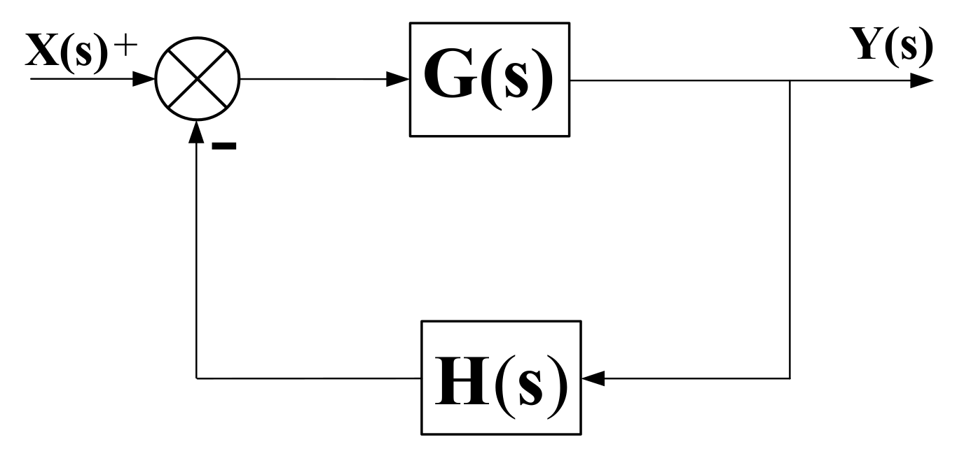
The Nyquist criterion is extended for the scalar transfer functions by MacFarlane and Postlethwaite in 1980. It is developed to a generalized Nyquist criterion to address the stability by a matrix transfer function. The generalized Nyquist criterion for the system shown in Figure 6 can be stated as follows:

The transfer function of this system is:

$$y(s)={[I+G(s)H(s)]}^{-1}G(s)x(s)$$

(35)

where $G(s)H(s)$ is defined as the return ratio of the system.

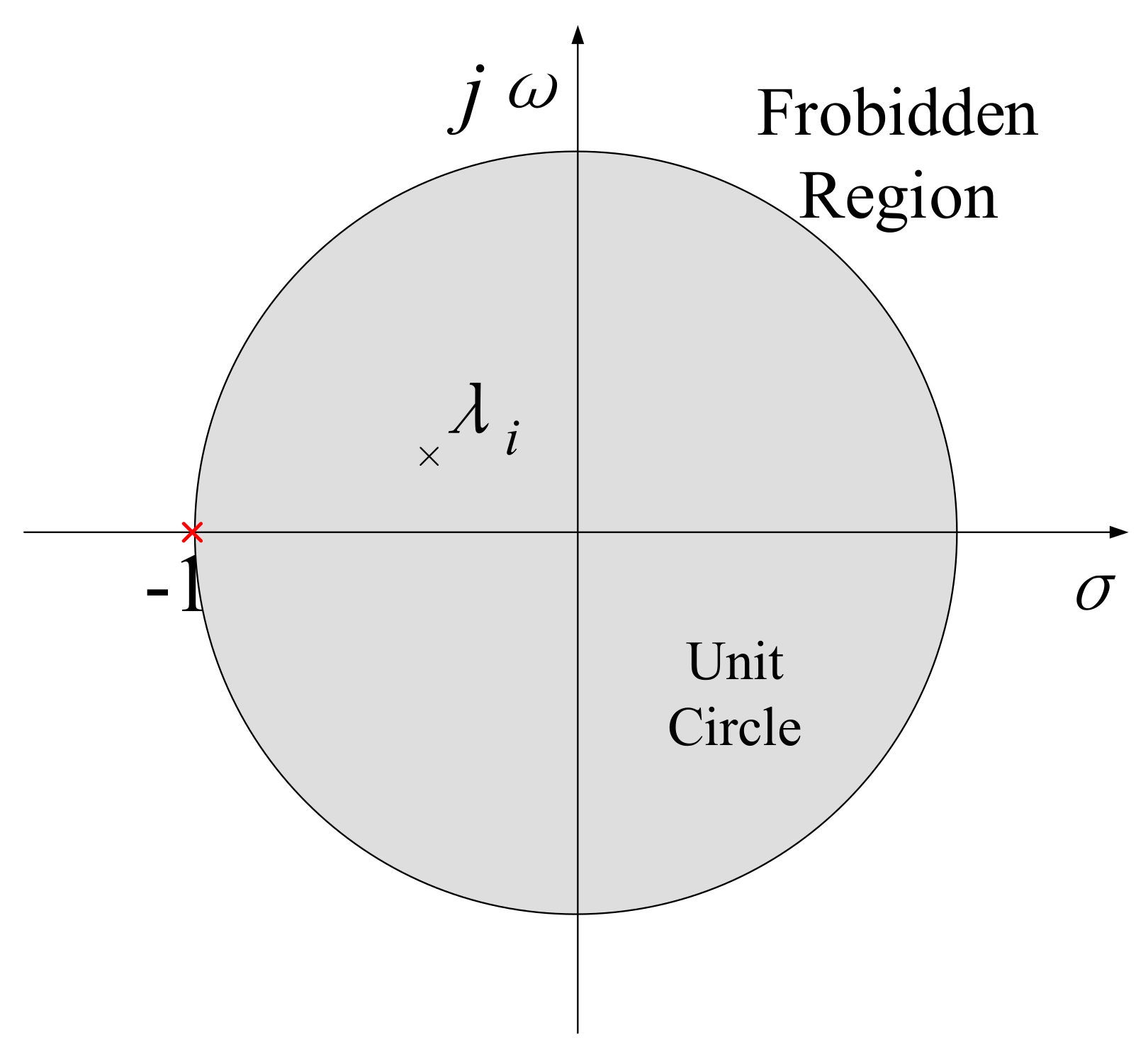
The assumption is made that the multivariable feedback system shown in Figure 6 have no open loop uncontrollable or unobservable modes whose corresponding characteristic frequencies lie in the right-half plane. Under this assumption, the system is stable if and only if the net sum of anti-clockwise encirclements of the critical point (−1,j0) by the set of characteristic loci of the return ratio $L(s)=G(s)H(s)$ is equal to the total number of right-half plane poles of $G(s)$ and $H(s)$. For this paper, the fast-charging station and power grid are stable, respectively, so the number of right-half panel poles for both the grid-side output impedance $Z_{s,dq}^{2m}$ and the fast-charging pile-side input admittance $Y_{s,dq}^{2m}$ is 0, that is, the number of right-half panel poles for the return ratio is 0. Thus, the interaction system is stable if the number of anti-clockwise encirclements of the point (−1,j0) by all eigenvalues of the return ratio is 0. Hence the eigenvalues of the return ratio should be located within the region of a unit circle as shown in Figure 7. The region out of the unit circle is regard as the forbidden region to guarantee the stability of the system.

In the fast-charging station system, the output impedance of the grid side $Z_{go,dq}^{2m}(s)$ is written as:

$$Z_{go,dq}^{2m}(s)=\left[\begin{array}{cc}{Z}_{dd}& Z_{dq}\\ Z_{qd}& Z_{qq}\end{array}\right]$$

(36)

The fast-charging pile-side input admittance is written as:

$$Y_{cl,dq}^{2m}(s)=\left[\begin{array}{cc}{Y}_{dd}& Y_{dq}\\ Y_{qd}& Y_{qq}\end{array}\right]$$

(37)

The return ratio is defined as:

$$L_{dq}^{2m}(s)=Z_{go,dq}^{2m}(s)\cdot Y_{cl,dq}^{2m}(s)=\left[\begin{array}{cc}{L}_{dd}& L_{dq}\\ L_{qd}& L_{qq}\end{array}\right]$$

(38)

On the basis of generalized Nyquist criterion, singular value criterion and norm criterion for cascade system in dq frame are developed.

According to the singular value criterion, the cascade system is stable if the product of the maximum singular value of the output impedance matrix of the grid-side system and the maximum singular value of the input admittance matrix of the converter-side is less than 1 in the whole frequency domain. In mathematics it can be expressed as follows:

$$\overline{\sigma }(Z_{s,dq}(s))\cdot \overline{\sigma }(Y_{s,dq}(s))<1$$

(39)

where $\overline{\sigma }$ is the maximum module of the singular value for a matrix.

As Equation (39) is satisfied, the eigenvalue of the return ratio $L_{dq}^{2m}(s)$ is surely located in the unit circle due to the module of eigenvalues being in the range determined by the module of the maximum and minimum singular values of a matrix. The mathematical explanation is proposed in Appendix B.

The norm criterion is easy for stability analysis of the cascade system due to its simplification, a modified norm criterion for the AC cascade system is proposed in [26] as follows:

$$({\Vert Y_{s,dq}(s)\Vert }_G\cdot {\Vert Z_{s,dq}(s)\Vert }_{sum}<1)\cup ({\Vert Y_{s,dq}(s)\Vert }_{sum}\cdot {\Vert Z_{s,dq}(s)\Vert }_G<1)$$

(40)

where the G norm and sum norm are defined as:

$$\begin{array}{l}{\Vert Y_{s,dq}(s)\Vert }_G=\max \left\{\left|Y_{dd}\right|,\left|Y_{dq}\right|,\left|Y_{qd}\right|,\left|Y_{qq}\right|\right\}\\ {\Vert Y_{s,dq}(s)\Vert }_{sum}=\left|Y_{dd}\right|+\left|Y_{dq}\right|+\left|Y_{qd}\right|+\left|Y_{qq}\right|\end{array}$$

(41)

3.2. Modified Forbodden Region-Based Criterion

The modified forbidden region-based criterion focuses on reducing the conservatism of the previously-proposed criterion. As shown in Figure 7, the forbidden region of the eigenvalue of $L_{dq}^{2m}(s)$ is the outside region of the unit circle. In this modified criterion, the forbidden region is reduced to the left half panel of the critical point (−1,j0) as shown in Figure 8.

The Gershgorin circle theorem is applied here to limit the distribution of the eigenvalues of $L_{dq}^{2m}(s)$ in the right-half panel of the point (−1,j0) as shown in Figure 9. According to the Gershgorin circle theorem, the eigenvalues of $L_{dq}^{2m}(s)$ are located in the circles determined by:

$$\begin{array}{l}\left|z-L_{dd}\right|=\left|L_{dq}\right|\\ \left|z-L_{qq}\right|=\left|L_{qd}\right|\end{array}$$

(42)

In order to guarantee the eigenvalues are not located in the forbidden region shown in Figure 8, the Gershgorin circle cannot cross with the forbidden region, that is, the left most point of the Gershgorin circle should not less than −1, so the following conditions have to be met:

$$\begin{array}{l}\mathrm{Re}(L_{dd})-\left|L_{dq}\right|>-1\\ \mathrm{Re}(L_{qq})-\left|L_{qd}\right|>-1\end{array}$$

(43)

According to [28], $L_{dq}^{2m}{}^T(s)$ and $L_{dq}^{2m}(s)$ have the same eigenvalues, and all the eigenvalues of $L_{dq}^{2m}(s)$ are also located in the Gershgorin circle of $L_{dq}^{2m}{}^T(s)$, that is:

$$\begin{array}{l}\mathrm{Re}(L_{dd})-\left|L_{qd}\right|>-1\\ \mathrm{Re}(L_{qq})-\left|L_{dq}\right|>-1\end{array}$$

(44)

Thus, when any one of the Equations (43) and (44) is satisfied, the system is stable. The stable criterion for this system is:

$$\left(\begin{array}{l}\mathrm{Re}(L_{dd})-\left|L_{dq}\right|>-1\\ \mathrm{Re}(L_{qq})-\left|L_{qd}\right|>-1\end{array}\right)\cup \left(\begin{array}{l}\mathrm{Re}(L_{dd})-\left|L_{qd}\right|>-1\\ \mathrm{Re}(L_{qq})-\left|L_{dq}\right|>-1\end{array}\right)$$

(45)

On the other hand, both $Z_{go,dq}^{2m}(s)$ and $Y_{cl,dq}^{2m}(s)$ have the same structure of:

$$\left[\begin{array}{cc}A(s)& B(s)\\ -B(s)& A(s)\end{array}\right]$$

(46)

Thus, the return ratio $L$ also have the same structure as mentioned above. It can be obtained:

$$\begin{array}{c}\left|L_{dq}\right|=\left|L_{qd}\right|\\ \mathrm{Re}(L_{dd})=\mathrm{Re}(L_{qq})\end{array}$$

(47)

Thus the stability criterion can be simplified and expressed as follows:

$$\mathrm{Re}(L_{dd})-\left|L_{dq}\right|>-1$$

(48)

4. Stability Analysis of the EV Fast-Charging Station

4.1. Parameters of the Fast-Charging Station System

The power grid-side subsystem in this paper generally contains four parts: the regional power grid, the substation distribution transformer, the distribution line (overhead line or underground cable), and the distribution transformer for the EV fast-charging station. The difference in any one of the four parts will affect the grid-side subsystem output impedance and then influence the fast-charging station stability. For the stability analysis, a standard condition is set as a contrast case. In this standard condition, the EV fast-charging station has five identical fast-charging piles. The related parameters of the main circuit are shown in

Table 1. Fast-charging pile main circuit parameters.

Category	Value
AC side voltage (Vg)	400 V
DC side voltage (Vdc)	600 V
Sampling period (Ts)	5 × 10−4 s
Filter inductance (Lf)	0.005 H
Filter conductance (Cf)	99 × 10−6 F
Switching frequency (fs)	2000 Hz
Grid fundmental frequency (f)	50 Hz

.

The control parameters of the current control loop are shown in

Table 2. Current loop control parameters.

Category	Value
Proportional gain (Kp)	0.15
Integral gain (Ki)	1.5

as follows:

The parameters of the power grid are shown in

Table 3. Power grid-side parameters.

Category	Value
Regional Short Circuit Capacity(S)	300 MVA
Ratio of inductance and reactance(kx/r)	15
10 kV feeder cable(Lfeeder)	2 km

:

The parameters of the transformers are shown in

Table 4. Parameters of the distribution transformers.

Category	Voltage Ratio	Capacity (MVA)	Short Circuit Power (kW)	Impedance Voltage
110 kV Transformer	110 kV/10 kV	20	88.4	10.5
10 kV Transformer	10 kV/0.4 kV	0.63	8.169	4.5

:

4.2. Power Grid Side Subsystem Influence Factors

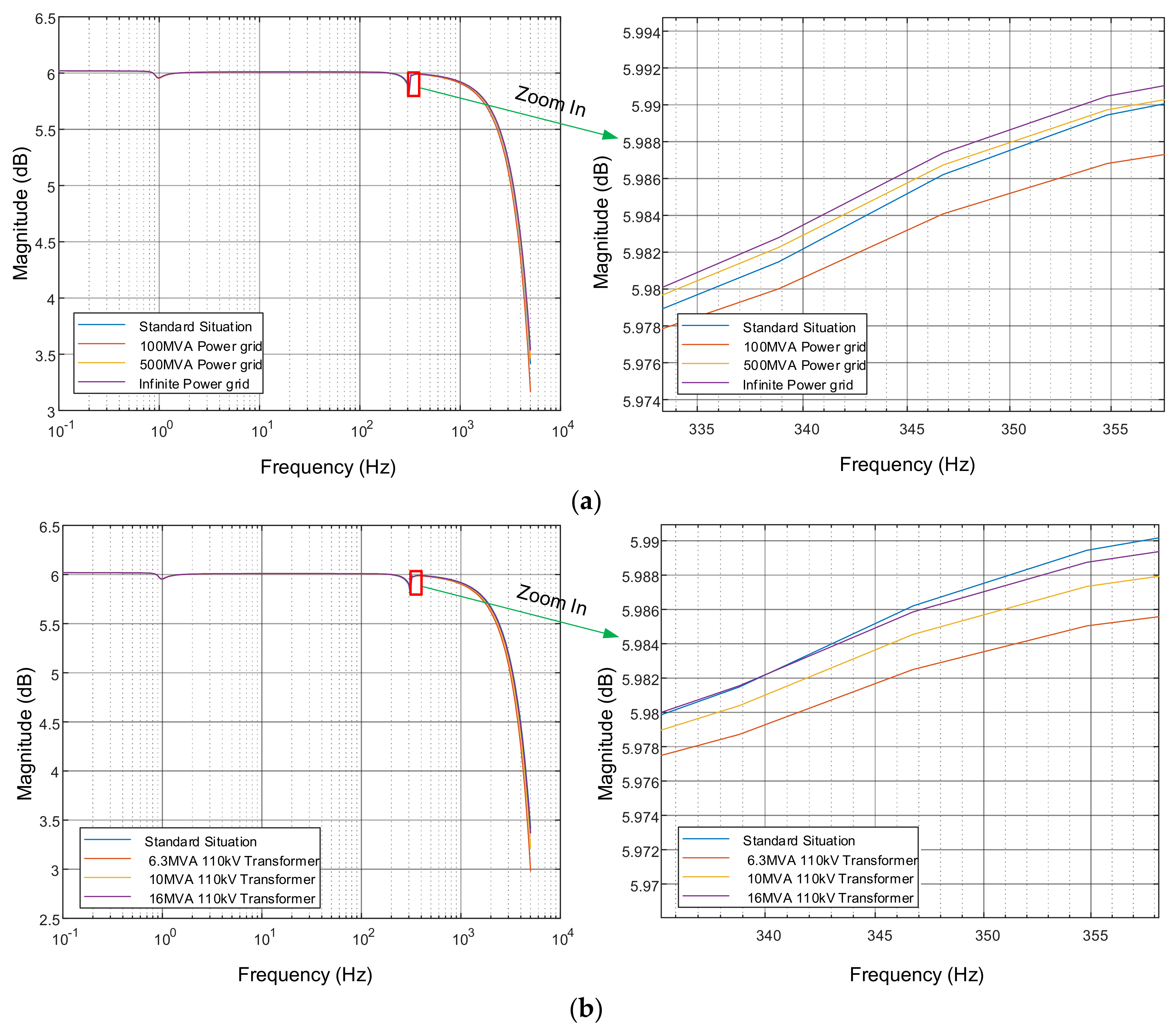
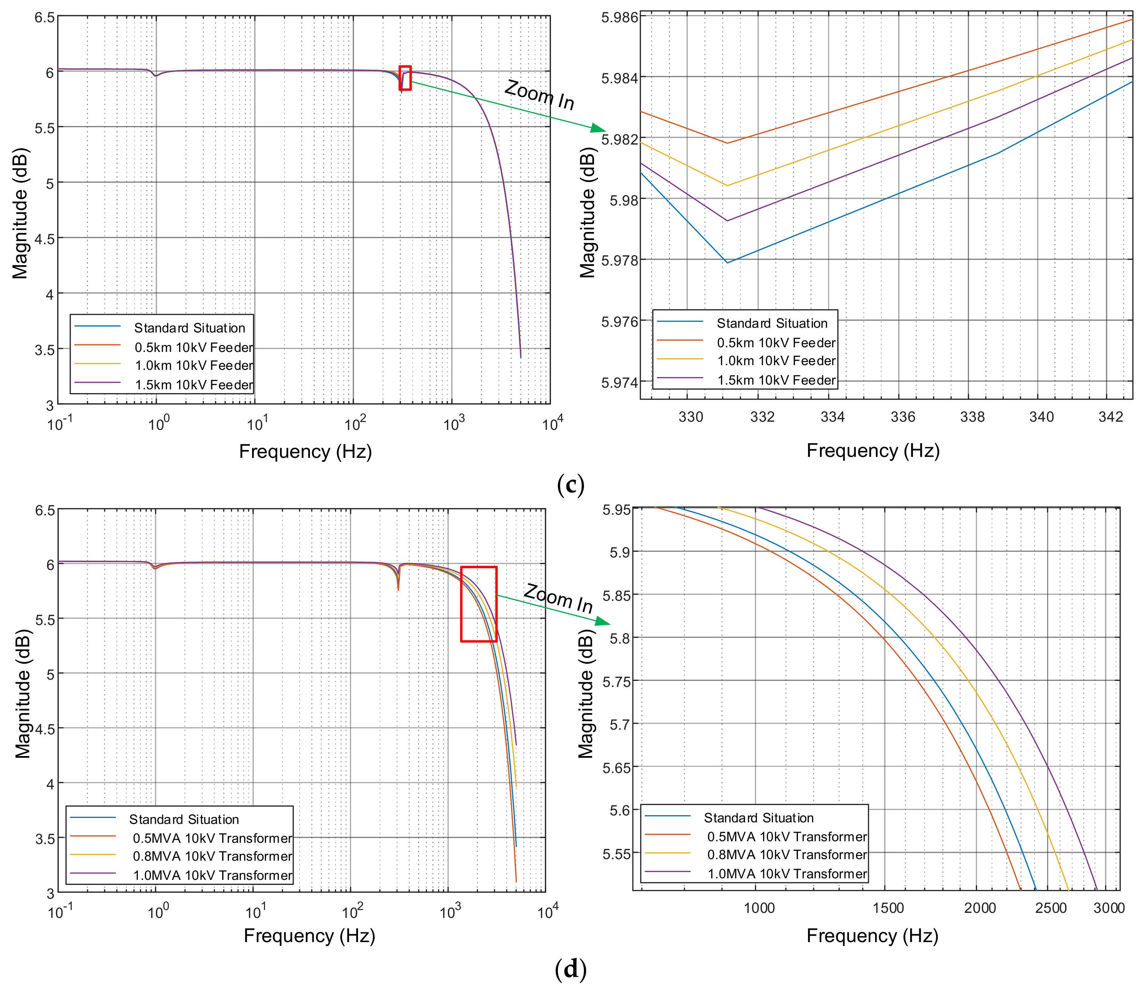
The relationship between the impedance of the grid side subsystem and the stability of the fast-charging station is investigated by regarding the four parts that constitute the grid-side subsystem as influence factors. Only one part is changed while the other parts are kept constant at each time to investigate the corresponding influence. The magnitude-frequency diagrams are shown in Figure 10.

Figure 10a shows the influence while the power grid short circuit capacity varies through 100 MVA–300 MVA–500 MVA–infinite. Figure 10b shows the influence while the 110 kV transformer capacity varies through 6.3 MVA–10 MVA–16 MVA–20 MVA. Figure 10c shows the influence while the 10 kV feeder length varies through 0.5 km–1 km–1.5 km–2 km. Figure 10d shows the influence, while the 10 kV transformer capacity varies through 0.5 MVA–0.63 MVA–0.8 MVA–1 MVA.

According to the magnitude-frequency diagrams, it can be obtained that when any one factor is changed, the corresponding magnitude of the stability criterion changed. As shown in Figure 10a, along with the increasing of regional power grid short circuit capacity, the magnitude margin of the system is getting larger, which means the interaction system is getting more stable. Similarly, as shown in Figure 10b–d, along with the increasing of 110 kV and 10 kV distribution transformer capacity and decreasing of the 10 kV feeder length, the magnitude margin of the system is also getting larger. The law of change summarized from the figure is shown in the following

Table 5. Fast-charging pile main circuit parameters.

Influence Factor	Variation	Stability	Grid Side Impedance
SSC	↑	↑	↓
ST110	↑	↑	↓
Lfeeder	↓	↑	↓
ST10	↑	↑	↓

The symbol ↑ in the table denotes the increase of influence factor variation, system stability, and grid-side output impedance. Similarly, the symbol ↓ denotes the decrease of these indices.

.

As shown in the table, no matter the increase of the power grid short circuit capacity, 110 kV transformer capacity and 10 kV transformer capacity, or the decrease of 10 kV feeder length will all lead to the improvement of the fast-charging system stability. Thus, it can be concluded that when the output impedance of the grid-side subsystem decreases, the system stability will be enhanced. On the other hand, when the grid-side output impedance decreases, it is generally regarded that the grid side is getting stronger.

4.3. Fast-Charging Pile-Side Influence Factors

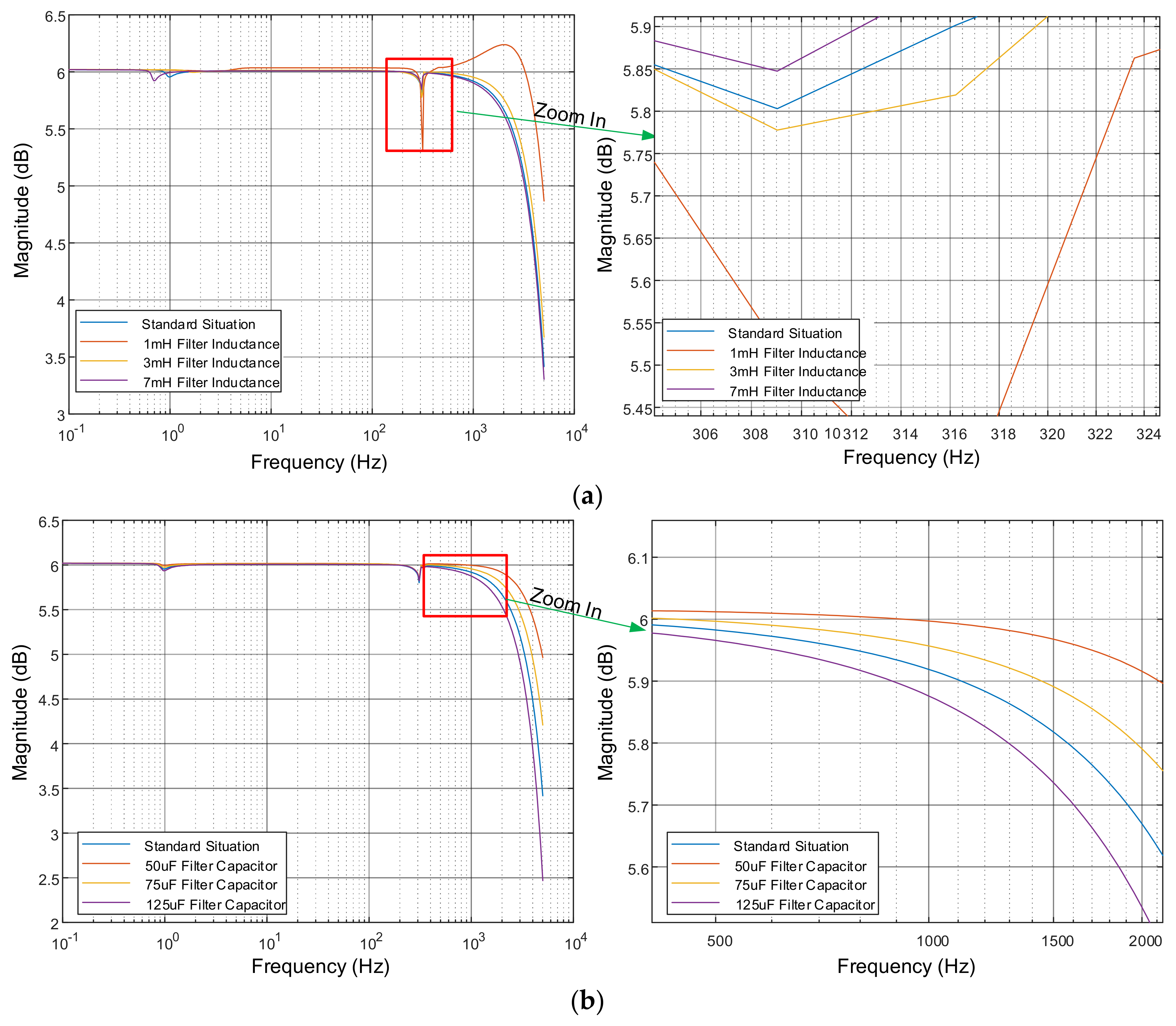
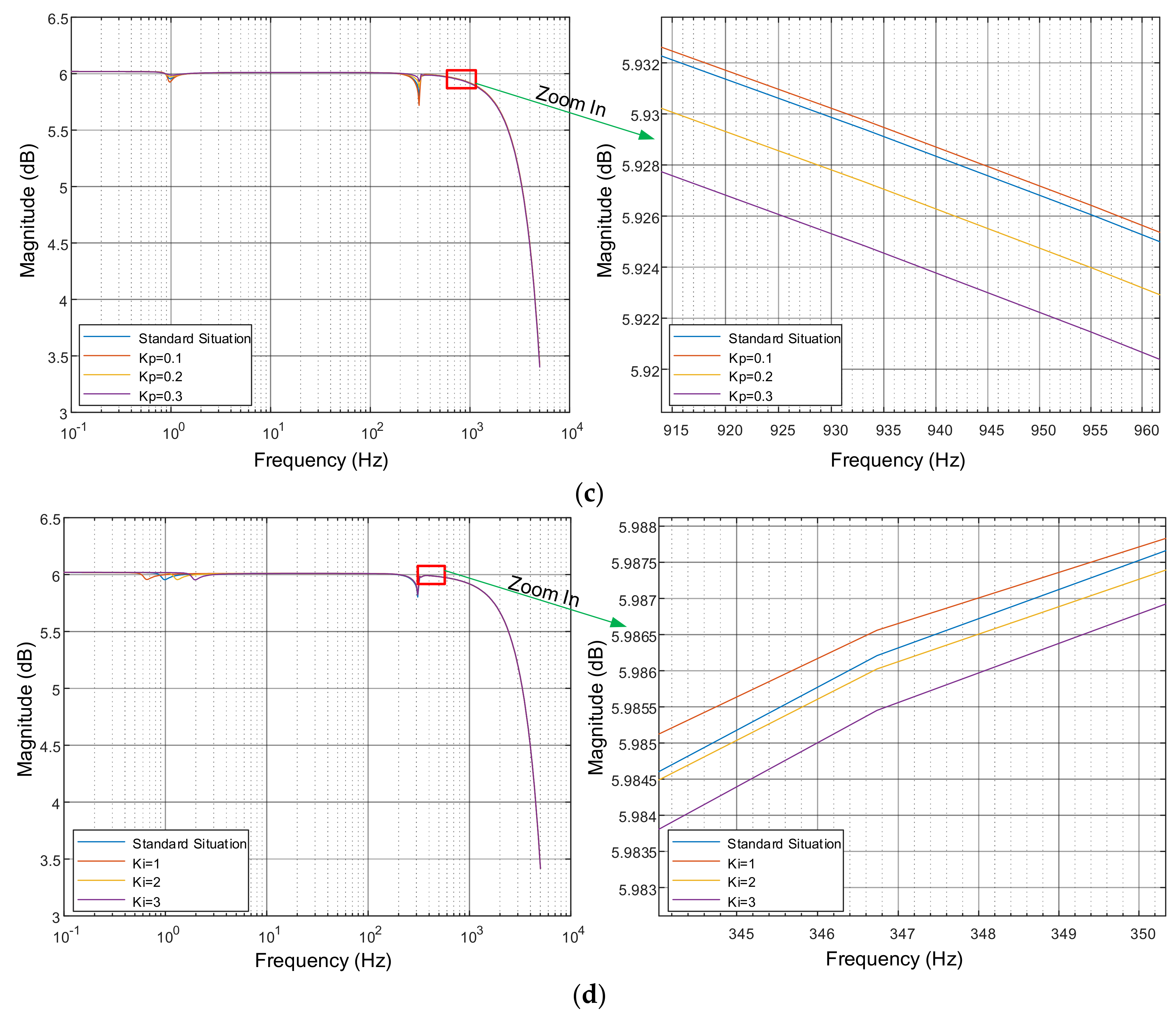
The input admittance of the fast-charging pile-side is derived from the current control loop. According to the input admittance model, the current controller parameters and the filter parameters all have influence on the input admittance. Thus, this part investigates the influence of these parameters on the fast-charging station stability. The corresponding magnitude-frequency diagrams are shown in Figure 11.

Figure 11a shows the influence while the filter inductor varies through 1 mH–3 mH–5 mH–7 mH. Figure 11b shows the influence while the filter conductor varies through 50 µF–75 µF–100 µF–125 µF. Figure 11c shows the influence while the proportional gain varies through 0.1–0.15–0.2–0.5. Figure 11d shows the influence while the integral gain varies through 1–1.5–2–3.

According to the magnitude-frequency diagrams, it can be obtained that when any one factor is changed, the corresponding magnitude of the stability criterion changed. The magnitude-frequency diagrams shown in Figure 11a,b depict the influence of filter parameters on the interaction system stability. According to Figure 11a, the magnitude margin increases along with the increasing of the filter inductance, while in Figure 11b, it is depicted that the stability margin decreases along with the increase in the filter conductance. The influence of the PI controller parameters are shown in Figure 11c,d, along with the increasing of the proportional factor and the integral factor, the stability margin of the interaction system decreases. The law of change summarized from the figure is shown in the following

Table 6. Fast-charging pile main circuit parameters.

Influence factor	Variation	Stability	Charging Pile Side Admittance
Lf	↑	↑	Uncertain
Cf	↑	↓	↑
Kp	↑	↓	Uncertain
Ki	↑	↓	Uncertain

The symbols ↑ and ↓ denote the same meaning as in Table 5.

.

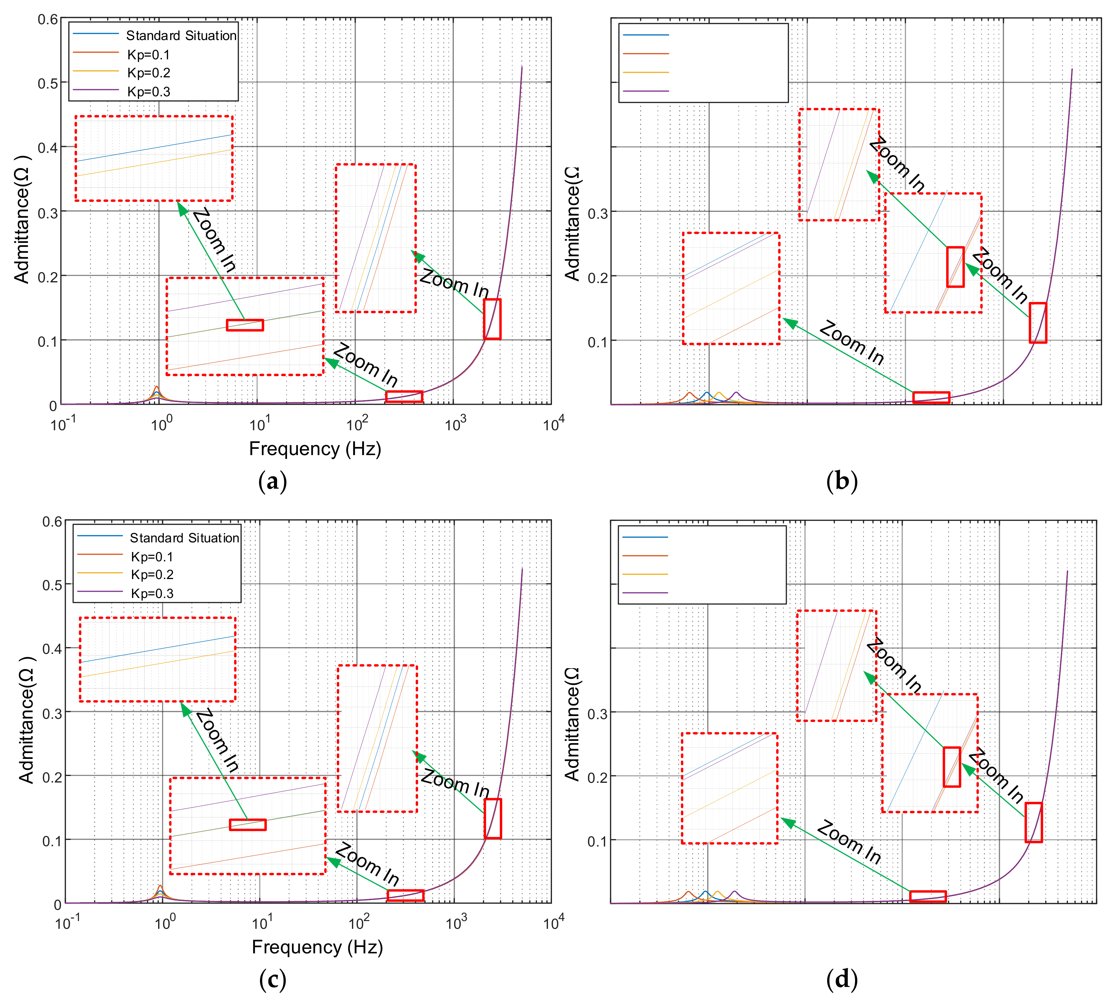
Along with the increase of the filter conductance, the proportional factor, and the integral factor, the stability margin of the fast-charging system decreases. The stability margin increases while the filter inductance increases. However, the charging pile-side input admittance variation tendency is difficult to determine since the expression of the input admittance is rather complex. The magnitude-frequency diagrams of the input admittance of the fast-charging system in these situations are shown in Figure 12.

According to the diagrams shown in Figure 12, the influence of the filter parameters and current loop control parameters on the input admittance is uncertain. In some frequency ranges, the relationship is a positive correlation, while in other frequency ranges, the relationship is a negative correlation. The input admittance derived from the current control loop is actually a complex transfer function, and it has different expression with the common impedance that is expressed by r + s·L, so the relationship is uncertain.

4.4. Time Domain Simulation

In order to verify the modeling and stability analysis method, time domain simulation is used in this section. In the simulation, the equal output impedance of the grid-side subsystem and the LC filter inductor are changed to investigate their influence on the PCC voltage. The voltage waveforms of the PCC while the output impedance of the grid-side subsystem changes are shown in Figure 13.

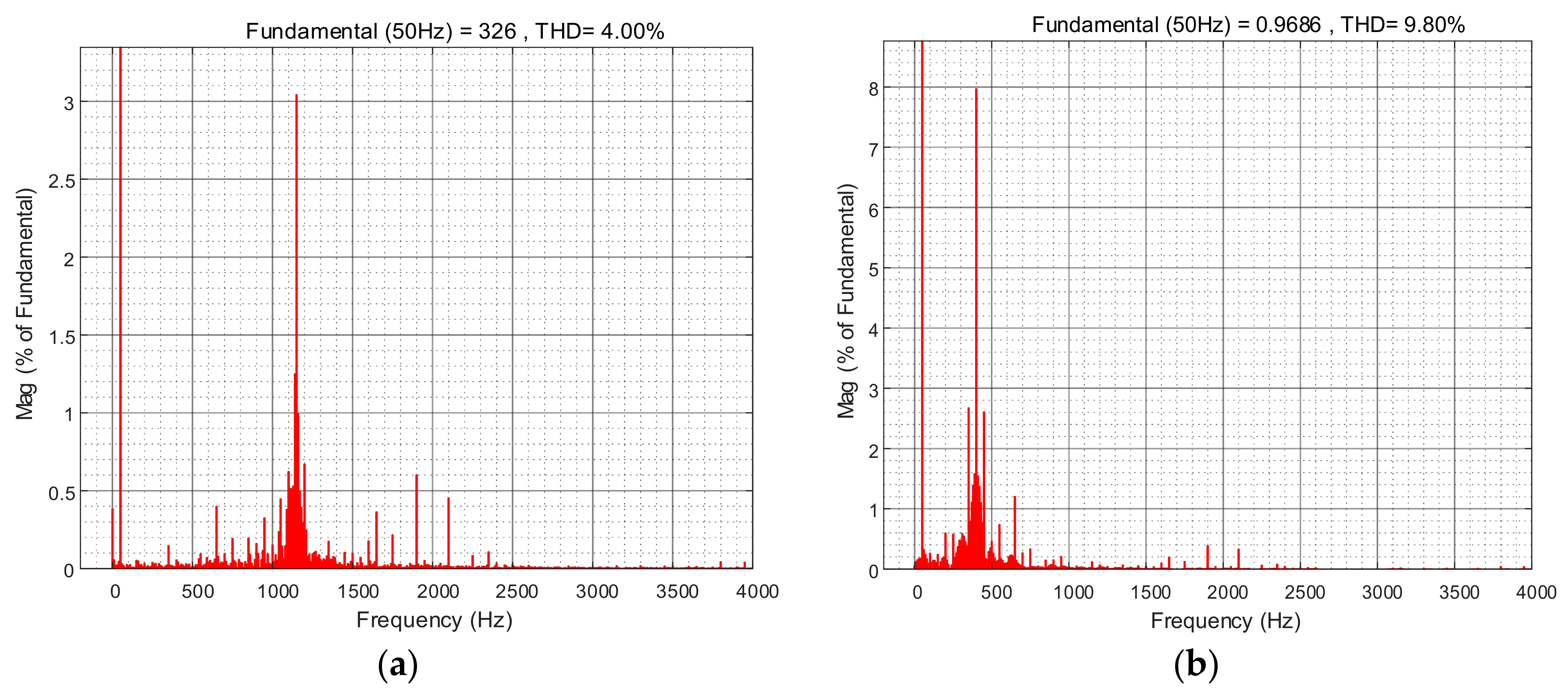
According to the waveform shown in Figure 13, as the output impedance increased to 10 times the original value, obvious distortion appears in the voltage waveform. From this point, the fast-charging system is becoming unstable when the output impedance increases. For more detailed information, the Fourier transformation is used to analysis the PCC voltage. The analysis result is shown in Figure 14.

As shown in the spectrum, the harmonics increase significantly as the grid-side output impedance increases. Since the output impedance of the grid-side subsystem increases, the grid side subsystem is relatively weak; this change leads to instability.

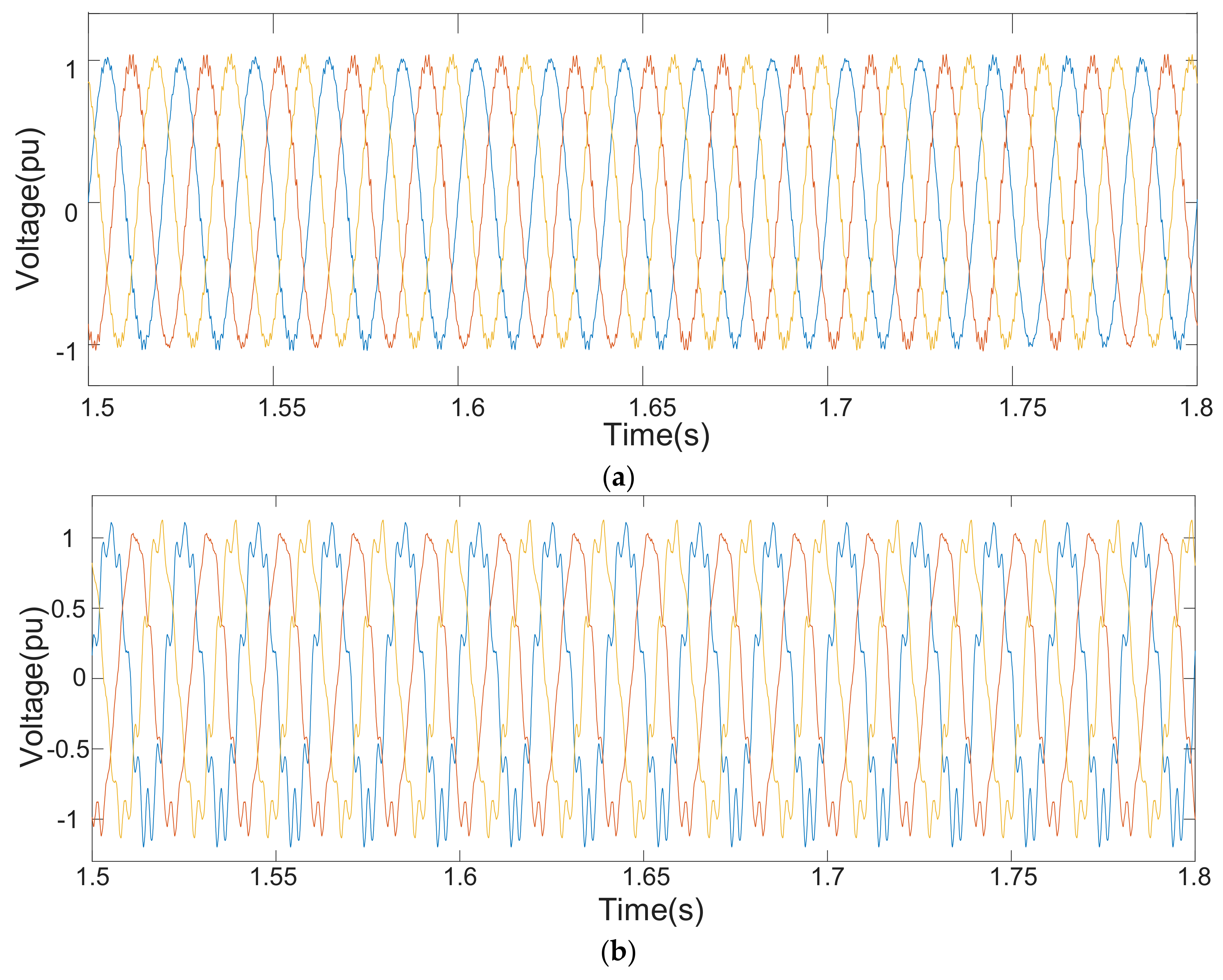
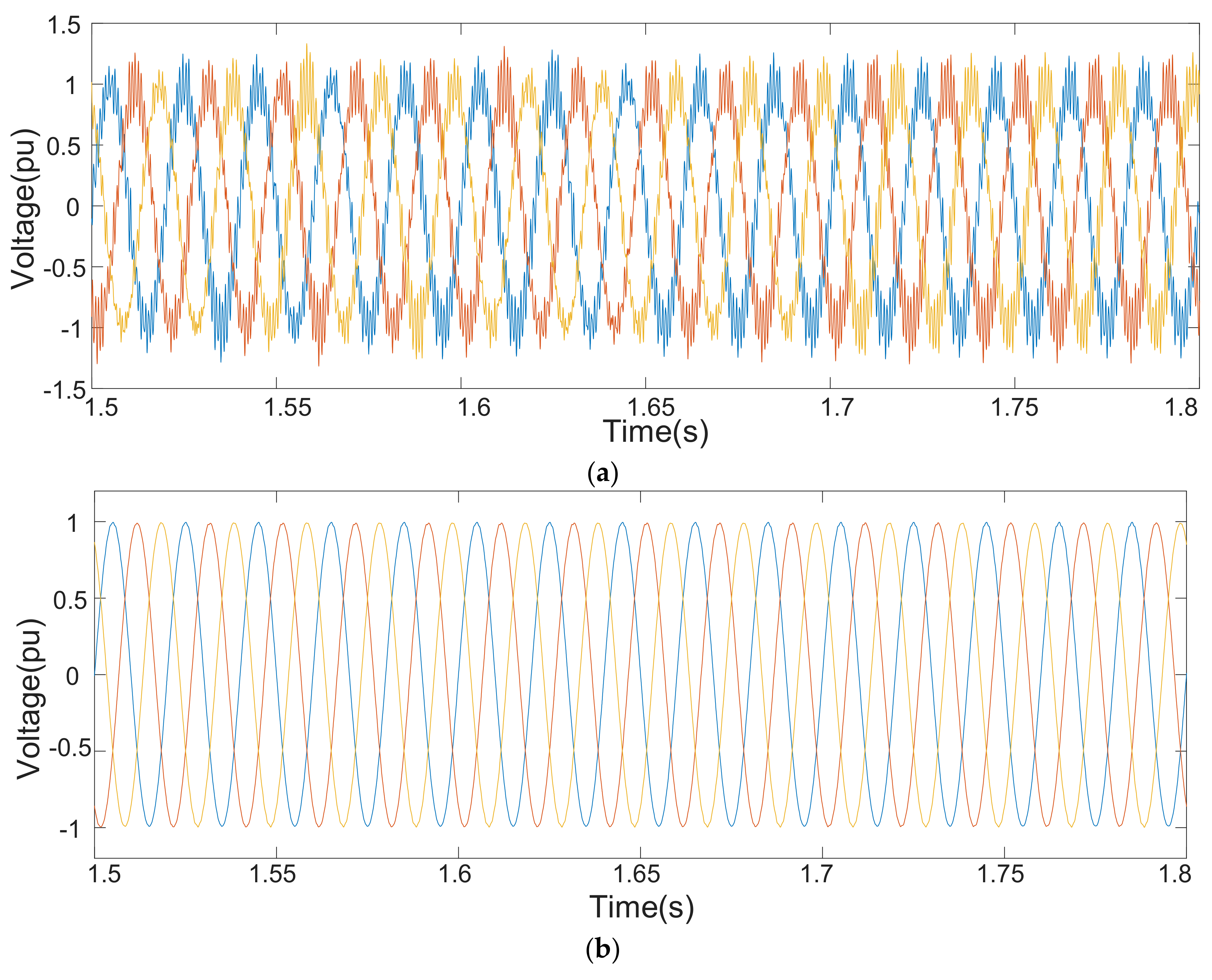
The voltage waveforms of PCC while the LC filter inductance changes are shown in Figure 15.

As the voltage waveform in the above picture shows, when the LC filter inductance decreases to 20% of the original value, the voltage waveform has serious distortion. When the LC filter inductance increases to 10 times the original value, the voltage waveform is very smooth. The time domain simulation depicts that the fast-charging system becomes stable along with the increase of the LC filter inductance.

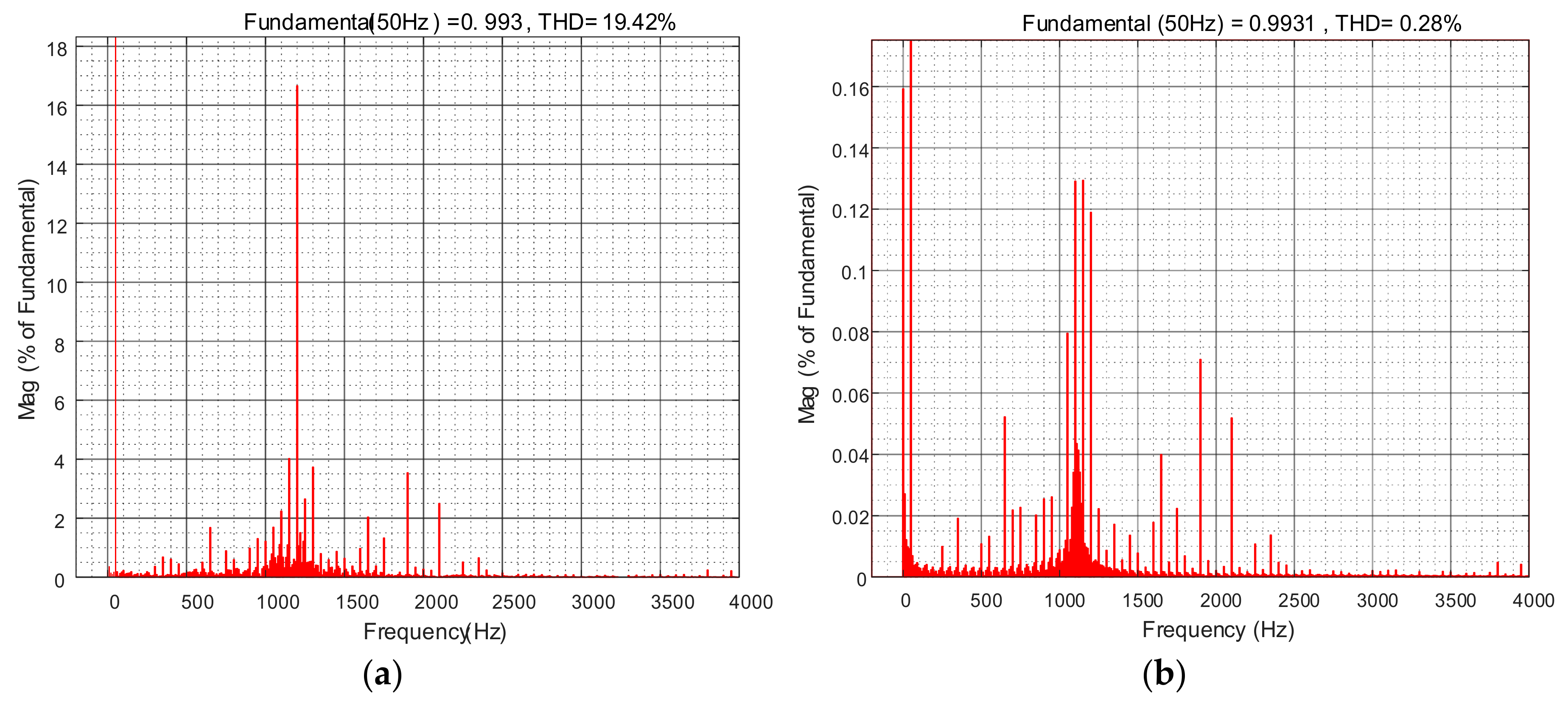
For a more detailed and quantitative analysis of the system stability, Fourier transformation is used to analyze the PCC voltage. The analysis result is shown in Figure 16.

According to the spectrum shown in Figure 16, the harmonics decrease significantly as the fast-charging pile LC filter inductance increases. Since the fast-charging pile LC filter inductance increases, harmonics are filtered out by the inductor, so the system is more stable and the PCC voltage waveform is smooth.

5. Conclusions

This paper analyzes the electric vehicle fast-charging station and power grid interaction system stability by using the impedance-based modeling method. In this method, the interaction system is separated into two parts: the source-side subsystem and the load-side subsystem. The source side subsystem is represented by the Thevenin equivalent model and the load side subsystem is represented by the input admittance.

The dynamic modeling approach of the electric vehicle fast-charging station in dq frame is proposed. The input admittance of the fast-charging station in matrix form of dq frame is derived from the current control loop by using the complex vector and complex transfer function. On the basis of the dynamic model of the fast-charging system, the forbidden region-based stability criterion is adopted for stability analysis. Some conclusions can be drawn as follows:

(1) The influence of the source-side and load-side parameters are analyzed by using the forbidden region-based stability criterion. Time domain simulation is provided to prove the proposed model and stability analysis method are reasonable.

(2) Parameters of both source-side and load-side can affect the stability of the interaction system. Different parameters have different influence tendencies.

References

- Yong, J.Y.; Ramachandaramurthy, V.K.; Tan, K.M.; Mithulananthan, N. A review on the state-of-the-art technologies of electric vehicle, its impacts and prospects. Renew. Sustain. Energy Rev. 2015, 49, 365–385. [Google Scholar] [CrossRef]
- China Plans to Ban Sales of Fossil Fuel Cars Entirely. Available online: https://techcrunch.com/2017/09/10/china-plans-to-ban-sales-of-fossil-fuel-cars-entirely/ (accessed on 11 September 2017).
- Green, R.; Staffell, I. Electricity in Europe: Exiting fossil fuels? Oxf. Rev. Econ. Policy 2016, 32, 282–303. [Google Scholar] [CrossRef]
- Sadeghi-Barzani, P.; Rajabi-Ghahnavieh, A.; Kazemi-Karegar, H. Optimal fast charging station placing and sizing. Appl. Energy 2014, 125, 289–299. [Google Scholar] [CrossRef]
- SAE Electric Vehicle and Plug in Hybrid Electric Vehicle Conductive Charge Coupler. Available online: https://www.sae.org/standards/content/j1772_201710/ (accessed on 13 October 2017).
- Gao, Y.; Ehsani, M. Investigation of battery technologies for the army’s hybrid vehicle application. In Proceedings of the 56th IEEE Conference on Vehicular Technology, Vancouver, BC, Canada, 24–28 September 2002; pp. 1505–1509. [Google Scholar]
- Zhan, Y.J.; Chan, C.C.; Chau, K.T. A novel sliding-mode observer for indirect position sensing of switched reluctance motor drives. IEEE Trans. Ind. Electron. 1999, 46, 390–397. [Google Scholar] [CrossRef] [Green Version]
- Williamson, S.S.; Rathore, A.K.; Musavi, F. Industrial electronics for electric transportation: Current state-of-the-art and future challenges. IEEE Trans. Ind. Electron. 2015, 62, 3021–3032. [Google Scholar] [CrossRef]
- Harnefors, L.; Wang, X.; Yepes, A.G.; Blaabjerg, F. Passivity-based stability assessment of grid-connected VSCs—An overview. IEEE J. Emerg. Sel. Top. Power Electron. 2016, 4, 116–125. [Google Scholar] [CrossRef]
- Ashabani, M.; Mohamed, Y.A.R.I.; Mirsalim, M.; Aghashabani, M. Multivariable Droop Control of Synchronous Current Converters in Weak Grids Microgrids with Decoupled dq-Axes Currents. IEEE Trans. Smart Grid 2015, 6, 1610–1620. [Google Scholar] [CrossRef]
- Wang, H.; Mingli, W.; Sun, J. Analysis of low-frequency oscillation in electric railways based on small-signal modeling of vehicle-grid system in dq frame. IEEE Trans. Power Electron. 2015, 30, 5318–5330. [Google Scholar] [CrossRef]
- Xiao, X.; Zhang, J.; Guo, C.; Yang, L. A new subsynchronous torsional interaction and its mitigation countermeasures. In Proceedings of the 2013 IEEE Conference on Energytech, Cleveland, OH, USA, 21–23 May 2013; pp. 1–5. [Google Scholar]
- Wang, L.; Xie, X.; Jiang, Q.; Liu, H.; Li, Y.; Liu, H. Investigation of SSR in practical DFIG-based wind farms connected to a series compensated power system. IEEE Trans. Power Syst. 2015, 30, 2772–2779. [Google Scholar] [CrossRef]
- Kwon, J.; Wang, X.; Blaabjerg, F.; Bak, C.L.; Sularea, V.S.; Busca, C. Harmonic Interaction Analysis in a Grid-Connected Converter Using Harmonic State-Space (HSS) Modeling. IEEE Trans. Power Electron. 2016, 32, 6823–6835. [Google Scholar] [CrossRef]
- Wen, B.; Boroyevich, D.; Burgos, R.; Mattavelli, P.; Shen, Z. Analysis of D-Q small-signal impedance of grid-tied inverters. IEEE Trans. Power Electron. 2016, 32, 675–687. [Google Scholar] [CrossRef]
- Cho, Y.; Hur, K.; Kang, Y.C.; Muljadi, E. Impedance-Based Stability Analysis in Grid Interconnection Impact Study Owing to the Increased Adoption of Converter-Interfaced Generators. Energies 2017, 10, 1355. [Google Scholar] [CrossRef]
- Aldhaheri, A.; Etemadi, A. Impedance Decoupling in DC Distributed Systems to Maintain Stability and Dynamic Performance. Energies 2017, 10, 470. [Google Scholar] [CrossRef]
- Cespedes, M.; Sun, J. Impedance modeling and analysis of grid-connected voltage-source converters. IEEE Trans. Power Electron. 2014, 29, 1254–1261. [Google Scholar] [CrossRef]
- Sun, J. Impedance-based stability criterion for grid-connected inverters. IEEE Trans. Power Electron. 2011, 26, 3075–3078. [Google Scholar] [CrossRef]
- MacFarlane, A.G.J. Complex Variable Methods for Linear Multivariable Feedback Systems; Taylor & Francis, Inc.: Oxfordshire, UK, 1980. [Google Scholar]
- Belkhayat, M. Stability Criteria for AC Power Systems with Regulated Loads. Ph.D. Thesis, Purdue University, West Lafayette, IN, USA, 1997. [Google Scholar]
- Chandrasekaran, S.; Borojevic, D.; Lindner, D. Input filter interaction in three-phase AC-DC converters. In Proceedings of the 30th Annual IEEE Conference on Power Electronics Specialists Conference, Charleston, SC, USA, 1 July 1999; pp. 987–992. [Google Scholar]
- Burgos, R.; Boroyevic, D.; Wang, F.; Karimi, K.; Francis, G. On the Ac stability of high power factor three-phase rectifiers. In Proceedings of the 2010 IEEE Conference on Energy Conversion Congress and Exposition (ECCE), Atlanta, GA, USA, 12–16 September 2010; pp. 2047–2054. [Google Scholar]
- Burgos, R.; Boroyevic, D.; Wang, F.; Karimi, K.; Francis, G. Ac stability of high power factor multi-pulse rectifiers. In Proceedings of the 2011 IEEE Conference on Energy Conversion Congress and Exposition (ECCE), Phoenix, AZ, USA, 17–22 September 2011; pp. 3758–3765. [Google Scholar]
- Mao, H.; Boroyevic, D.; Lee, F. Novel reduced-order small-signal model of a three-phase PWM rectifier and its application in control design and system analysis. IEEE Trans. Power Electron. 1998, 13, 511–521. [Google Scholar]
- Liu, F.; Liu, J.; Zhang, H.; Xue, D.; Hasan, S.U.; Zhou, L. Modified norm type stability criterion for cascade AC system. In Proceedings of the 2013 IEEE Conference on Energy Conversion Congress and Exposition (ECCE), Denver, CO, USA, 15–19 September 2013; pp. 442–447. [Google Scholar]
- Bo, W.; Boroyevich, D.; Burgos, R.; Mattavelli, P.; Zhiyu, S. D-Q impedance specification for balanced three-phase AC distributed power system. In Proceedings of the 2015 IEEE Conference on Applied Power Electronics Conference and Exposition (APEC), Charlotte, NC, USA, 15–19 March 2015; pp. 2757–2771. [Google Scholar]
- Liao, Y.; Liu, Z.; Zhang, G.; Xiang, C. Vehicle-Grid System Modeling and Stability Analysis with Forbidden Region-Based Criterion. IEEE Trans. Power Electron. 2017, 32, 3499–3512. [Google Scholar] [CrossRef]
- Wang, X.; Blaabjerg, F.; Wu, W. Modeling and Analysis of Harmonic Stability in an AC Power-Electronics-Based Power System. IEEE Trans. Power Electron. 2014, 29, 6421–6432. [Google Scholar] [CrossRef]
- Harnefors, L. Modeling of three-phase dynamic systems using complex transfer functions and transfer matrices. IEEE Trans. Ind. Electron. 2007, 54, 2239–2248. [Google Scholar] [CrossRef]
- Wang, X.; Harnefors, L.; Blaabjerg, F. Unified Impedance Model of Grid-Connected Voltage-Source Converters. IEEE Trans. Power Electron. 2017, 33, 1775–1787. [Google Scholar] [CrossRef]
Figure 1.
Single-line sketch map of fast-charging station connection to the power grid.
Figure 2.
Fast-charging pile electrical topology diagram.
Figure 3.
Simplified block diagram of the three-phase fast-charging pile.
Figure 4.
Block diagram of the inner current control loop.
Figure 5.
Source-side subsystem Thevenin equal circuit.
Figure 6.
Matrix transfer function feedback system.
Figure 7.
Distribution of eigenvalues of the Ldq determined by the generalized Nyquist criterion.
Figure 8.
Forbidden region criterion for stability analysis.
Figure 9.
Gershgorin circle theorem-based eigenvalues distribution.
Figure 10.
The magnitude-frequency of stability criterion under different situations of the grid-side subsystem. (a) Regional power grid with different short circuit capacity; (b) 110 kV distribution transformer with different capacity; (c) 10 kV feeder with different length; and (d) 10 kV charging station transformer with different capacity.
Figure 11.
The magnitude-frequency of stability criterion under different situation of the fast-charging pile-side subsystem. (a) Different filter inductance of the fast-charging pile; (b) different filter capacitance of the fast-charging pile; (c) different proportional factor of the current control loop; and (d) different integral factor of the current control loop.
Figure 12.
The admittance-frequency diagram of fast-charging pile-side input admittance. (a) Input admittance of different inductors; (b) input admittance of different capacitors; (c) input admittance of different proportion factors; and (d) input admittance of different integral factors.
Figure 13.
The PCC voltage waveform of different grid-side output impedances. (a) Grid-side output impedance with the original value; and (b) the grid-side output impedance with 10 times the original value.
Figure 14.
The PCC voltage Fourier analysis for different grid side output impedance. (a) FFT for the original output impedance; and (b) FFT for 10 times the output impedance.
Figure 15.
The PCC voltage waveform of different LC filter inductance values. (a) Fast-charging pile LC filter inductance with 20% the original value; and (b) the fast-charging pile LC filter inductance with 10 times the original value.
Figure 16.
The PCC voltage Fourier analysis of different LC filter inductor values. (a) FFT for 20% the LC filter inductance; and (b) FFT for 10 times the LC filter inductance.