Optimal Design and Real Time Implementation of Autonomous Microgrid Including Active Load

Abstract

Controller gains and power-sharing parameters are the main parameters affect the dynamic performance of the microgrid. Considering an active load to the autonomous microgrid, the stability problem will be more involved. In this paper, the active load effect on microgrid dynamic stability is explored. An autonomous microgrid including three inverter-based distributed generations (DGs) with an active load is modeled and the associated controllers are designed. Controller gains of the inverters and active load as well as Phase Locked Loop (PLL) parameters are optimally tuned to guarantee overall system stability. A weighted objective function is proposed to minimize the error in both measured active power and DC voltage based on time-domain simulations. Different AC and DC disturbances are applied to verify and assess the effectiveness of the proposed control strategy. The results demonstrate the potential of the proposed controller to enhance the microgrid stability and to provide efficient damping characteristics. Additionally, the proposed controller is compared with the literature to demonstrate its superiority. Finally, the microgrid considered has been established and implemented on real time digital simulator (RTDS). The experimental results validate the simulation results and approve the effectiveness of the proposed controllers to enrich the stability of the considered microgrid.

1. Introduction

Nowadays, different distributed generation (DG) resources—such as wind and photovoltaic arrays (PVs)—are being rapidly connected in the utility grid to overcome the environmental problems and global warming gas emissions [1]. To operate a microgrid at the distribution level, constant impedance loads (CILs) and constant power loads (CPLs) are connected with DGs [2,3,4,5,6,7,8,9,10,11,12,13,14]. For inverter-based microgrids, stability analysis is one of the most important concerns [4,5,6,7,8]. In an autonomous microgrid, achieving accurate power-sharing while regulating the magnitude and the frequency of the microgrid is the main DGs control objective [4]. For enhancing and improving microgrid dynamic performance, researchers have used different centralized and decentralized control schemes [8,9,10,11,12]. The schemes advantages and disadvantages have been shortened in [8]. Different centralized control schemes to coordinate between parallel multiple inverters and to maximize the DGs productions and power exchanges of a microgrid with the main grid [8,9]. Centralized control in remote areas with long distance between inverters is impractical and costly to maintain a communication link [9]. Therefore, decentralized schemes are used to avoid the communication link cost [10,11]. These schemes are mostly based on the droop concept. Through droop control, emulating synchronous generators, sharing powers between inverter-based DGs was firstly proposed [6]. Droop control schemes with many advantages such as flexibility, redundancy, and expandability can be categorized for four main groups: (1) conventional and variants of the droop control [6,13]; (2) virtual framework structure-based method [14,15]; (3) “construct and compensate” based methods [16,17]; and (4) the hybrid droop/signal injection method [18,19]. The details and characters of various control schemes were illustrated in [5]. Another updated revision for the power-sharing schemes was presented in [20]. It was stated that load demand and the controller power-sharing coefficients dominantly distress the low frequency modes; while filter parameters, load dynamics, and the controller parameters of the inner voltage and outer current controllers distress the medium and high frequency damped modes [5]. Moreover, constant load perturbation and load dynamics significantly distress microgrid stability [3,21]. Considering CPLs and/or CILs, it is essential to understand microgrid dynamic behavior [22]. With similar frequency range, control loop dynamic of the inverter and negative incremental resistance are the main important characteristics of the CPLs [12]. These properties reduce the system damping especially when CPL consumes a significant portion of the power [23]. Behind that, active load needs to be synchronized with the microgrid. Phase locked loop (PLL) is used for synchronization [24,25]. Difficult tuning of the PLL parameters and its negative effect on the controller performance are almost the main PLL drawbacks [24]. Moreover, the coupling effect and interactions between the PLL itself and the system impedance lead to a potential instability issue [25]. Therefore, studying microgrid stability considering CPLs is very important [26,27,28,29,30,31]. Large-signal study is used to explore the microgrid stability with CPL [29,30,31]. A traditional Proportional Integral (PI) controller has been extensively used to control the DG inverters [29]. Many studies show that fixed-gain PI controllers cannot easily acclimate to load changes and disturbances, especially in large microgrids [30]. Many trial-and-error-based studies have significant drawbacks such as optimal settings difficulties and being time-consuming [12,32,33]. In [12], the analysis revealed that when the active load DC-voltage controller is designed with large gains, the voltage controller of the inverter becomes unstable. In addition, the controller design problem cannot be solved systematically. Recently, different computational intelligence techniques, like particle swarm optimization (PSO), have been used for different power system problems with impressive achievement [34]. Although, complexity of the control system will be increased with these algorithms, PSO advantages—like computational efficiency, simplicity, and robustness—will enhance the microgrid transient performance [3,35,36]. To study and analysis the power system dynamics, offline simulation such as MATLAB is not enough especially if the power converters with high switching frequency are included. Nowadays, real time digital simulator (RTDS) with many advantages like well-established real time simulation, fast, reliable, accurate, and cost effective study of complex power systems is used for prototyping and hardware-in loop testing [37]. Microgrid test beds were implemented in the laboratory to study control strategies, unbalanced problems, and optimal structures of distributed generation microgrids [38,39].

This paper examines microgrid dynamic stability considering active load. Current, voltage, and power controllers are used to control the voltage and current of the inverter-based DGs and to share the DGs output powers. Additionally, ac current and dc voltage of the active load are controlled using two PI controllers. This paper is a modest contribution to the ongoing discussions on the degradation of the dynamic performance of the microgrid considering active load. To best of our knowledge, this is the first study to investigate the microgrid stability including active load using heuristic techniques such as PSO. The authors’ attention has focused not only on achieving the microgrid stability but also on obtaining the optimal parameters. The paper has introduced a new approach to get the all parameters that affect the microgrid dynamic stability including active load. An optimal control technique is proposed. By minimizing the error deviations in the measured active power of the DG and the dc voltage of the active load, the control problem is optimally designed. To assess the effectiveness of the proposed optimal control, the considered microgrid has been modeled in MATLAB. In both ac and dc sides, different disturbances are applied to investigate the optimal control effectiveness on the microgrid stability. Comparison between the proposed controller and literature is investigated to prove its superiority. Finally, the considered microgrid has been established and implemented in a real time digital simulator (RTDS). The experimental results validate the simulation results and approve the effectiveness of the proposed controllers to enrich the stability of the considered microgrid.

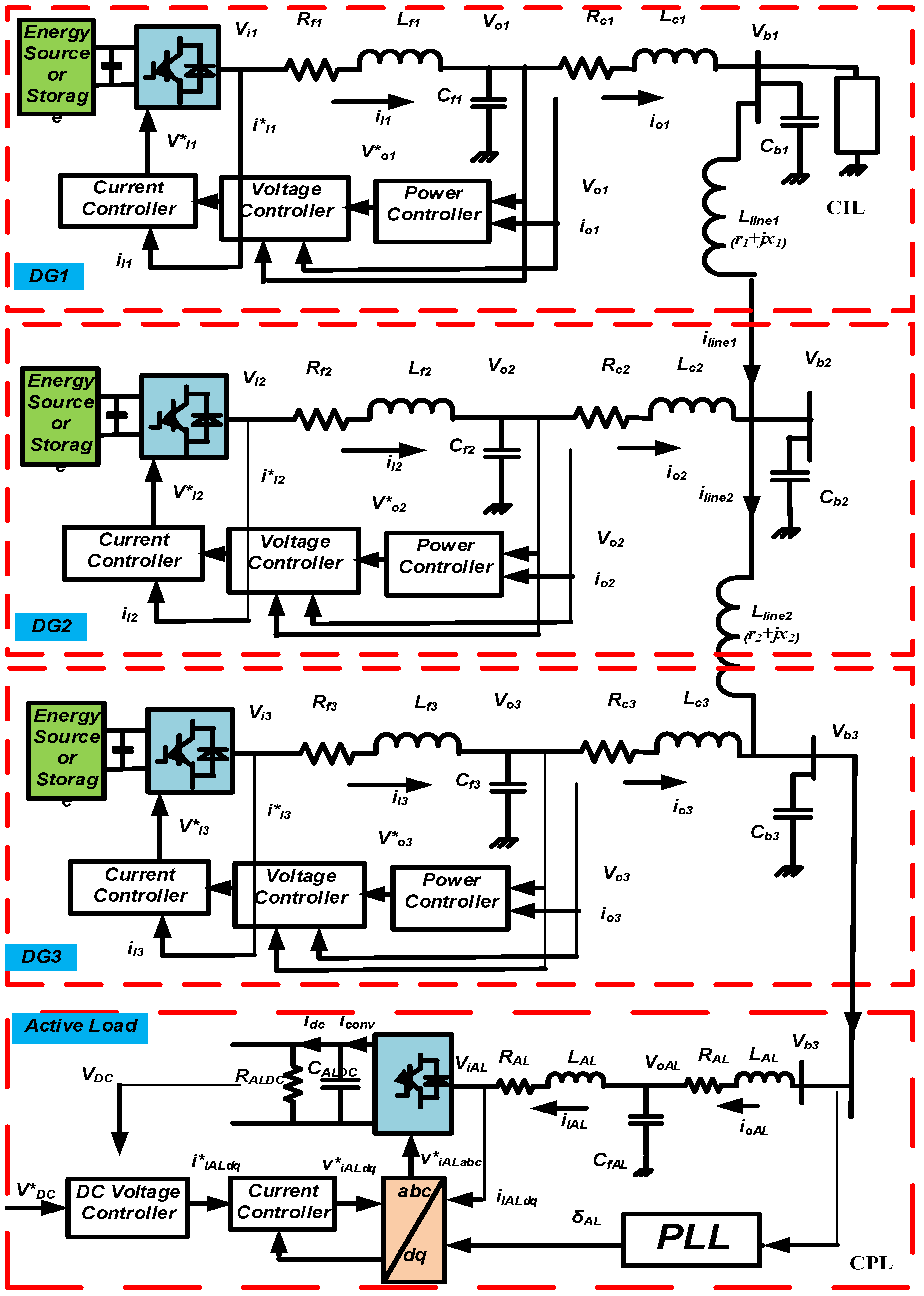
2. System Description

This section reviews the microgrid mathematical model of including the active load [3,12].

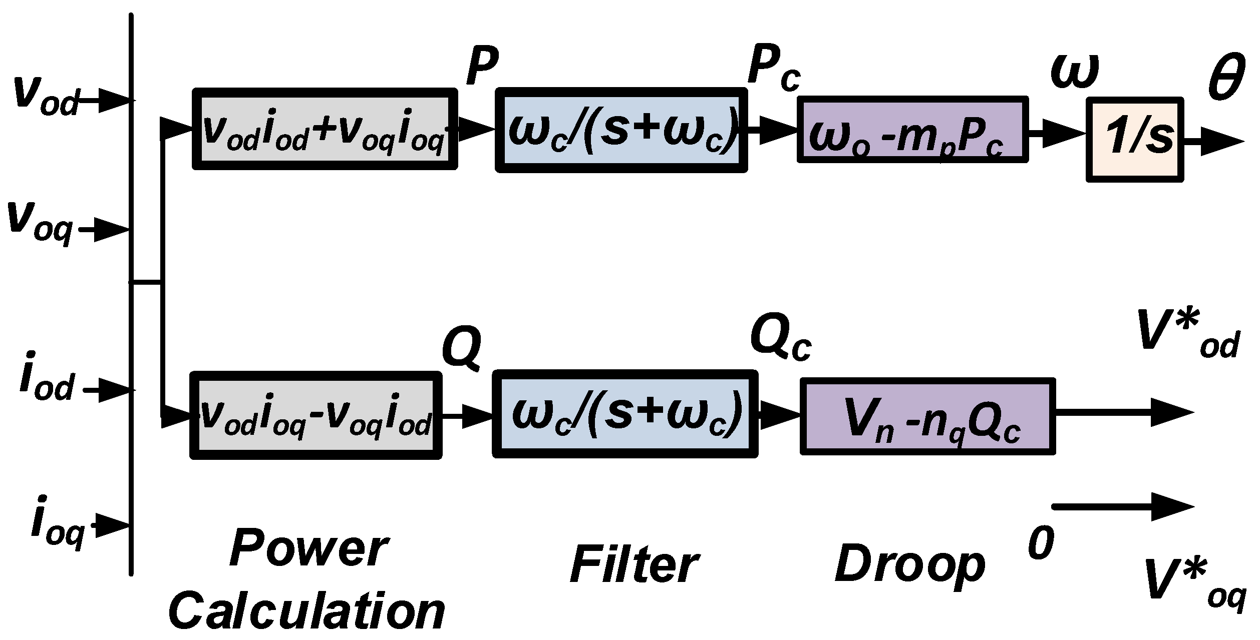
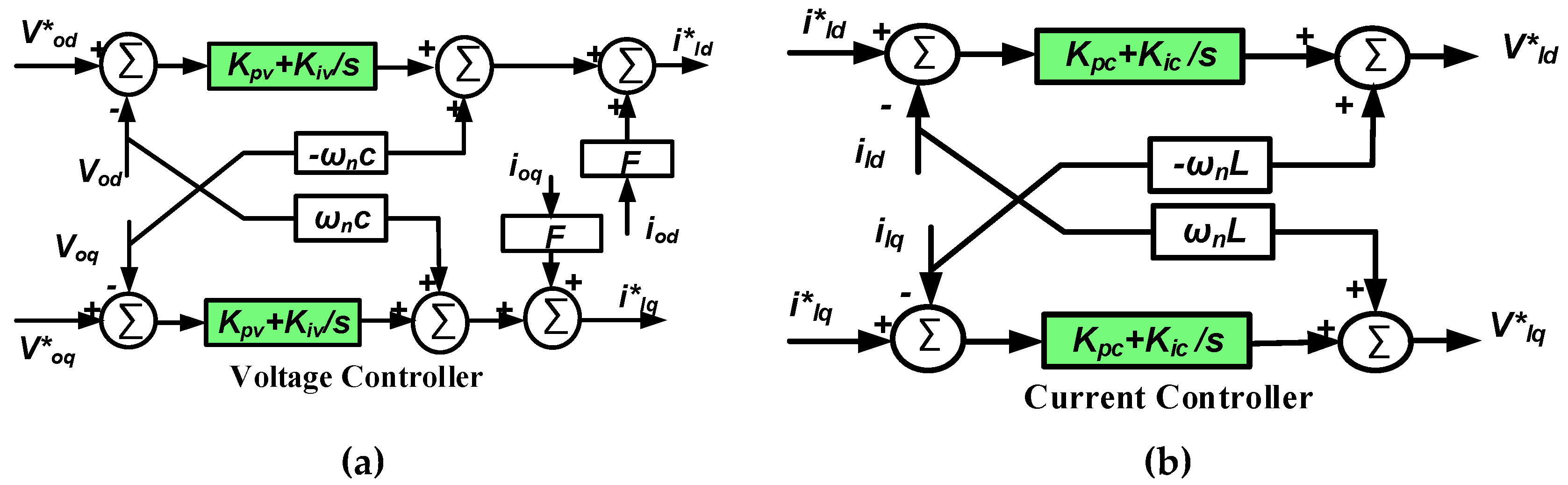
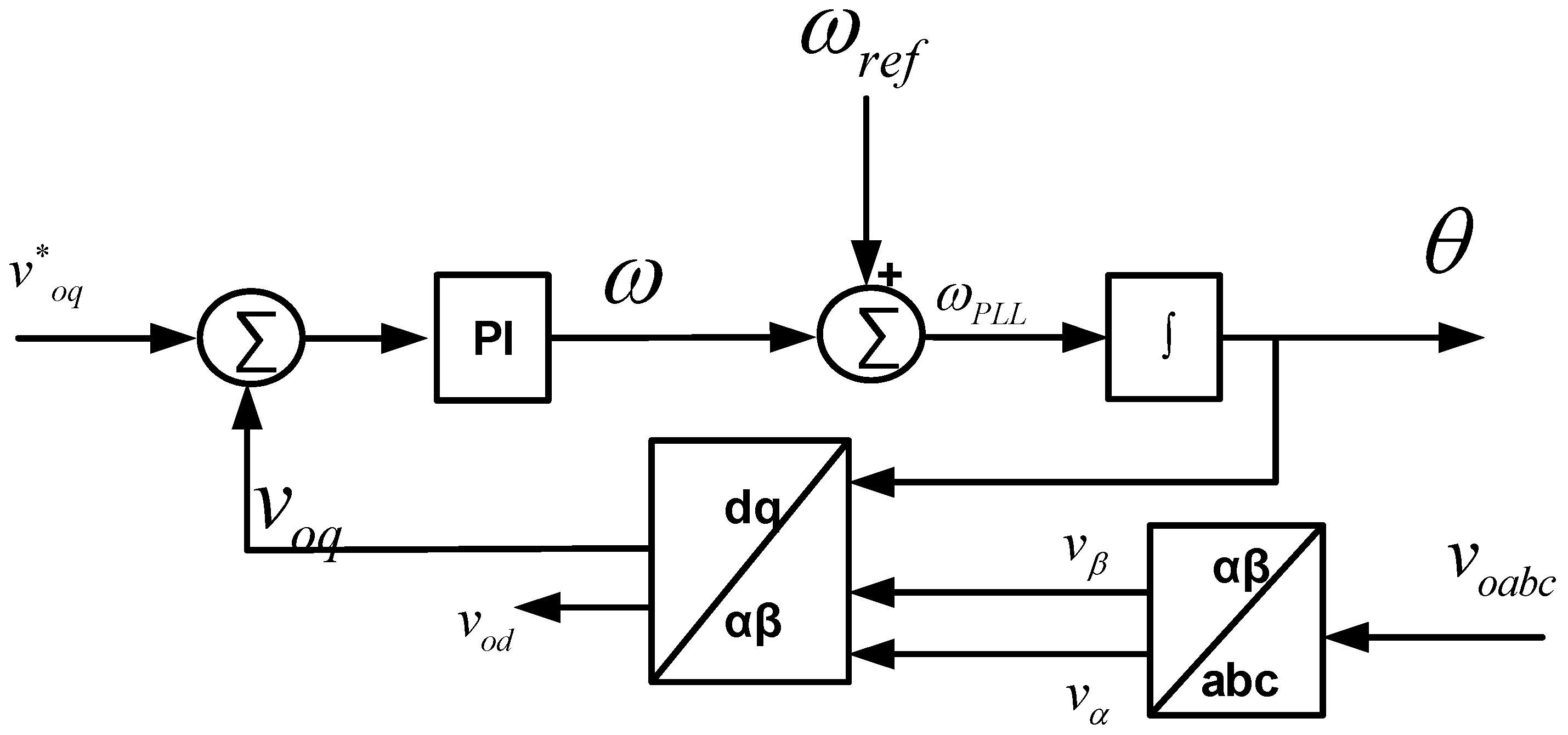
2.1. Autonomous Microgrid Model

Three inverter-based DGs are feeding two loads (CPL and CIL) through two transmission lines filters and coupling inductances as illustrated in Figure 1. In the autonomous mode, feeding the load with the predefined frequency and voltage values is the main objective of the inverter controller. Therefore, three controllers have been used to achieve this goal. Three controllers are presented to control the three inverters of the DG units. Firstly, emulating the synchronous generator, droop control is used to share the powers between DGs as given in Figure 2. Secondly, two PI controllers are employed to control the DGs’ output voltage and current as shown in Figure 3. It is worth mentioning that each DG inverter is assumed to be connected to a constant dc power source, so there no need to regulate the dc-link voltage otherwise, a controller should be introduced to regulate the dc-link voltage [40]. Meanwhile, our objective in this paper is to study the dynamic performance of the ac side of the inverter-based DG. The instantaneous real (P_m) and reactive powers (Q_m) are calculated using measured output current (i_o) and output voltage (v_o) is used to obtain the as given

$$P_m=v_{od}{i}_{od}+v_{oq}{i}_{oq}$$

(1)

$$Q_m=v_{od}{i}_{oq}-v_{oq}{i}_{od}$$

(2)

The average real P_c and reactive powers Q_c are obtained using a low pass filter as given in Figure 2.

$$P_c=\frac{{\omega }_c}{{\omega }_c+s}{P}_m, Q_c=\frac{{\omega }_c}{{\omega }_c+s}{Q}_m$$

(3)

where ω_c is the cut-off frequency of the low-pass filter.

As shown in Figure 2, the frequency ω is obtained from the active power while the d-axis reference voltage $v_{od}^{\ast }$ is obtained from the reactive power as

$$\omega ={\omega }_n-m_p{P}_c,\stackrel{•}{\theta }=\omega$$

(4)

$$v_{od}^{\ast }=V_n-n_q{Q}_c,v_{oq}^{\ast }=0$$

(5)

where ω_n is the nominal angular frequency of DG, V_n is the nominal magnitude of the DG voltage and m_p and n_q are the droop controller gains.

Voltage and current controllers’ state equations are shown

$$\begin{array}{l}{i}_{ld}^{\ast }=F{i}_{od}-{\omega }_n{C}_f{v}_{oq}+K_{pv}(v_{od}^{\ast }-v_{od})+K_{iv}{\displaystyle \int (v_{od}^{\ast }-v_{od})dt}\\ i_{lq}^{\ast }=F{i}_{oq}+{\omega }_n{C}_f{v}_{od}+K_{pv}(v_{oq}^{\ast }-v_{oq})+K_{iv}{\displaystyle \int (v_{oq}^{\ast }-v_{oq})dt}\end{array}$$

(6)

$$\begin{array}{l}{v}_{id}^{\ast }=-{\omega }_n{L}_f{i}_{lq}+K_{pc}(i_{ld}^{\ast }-i_{ld})+K_{ic}{\displaystyle \int (i_{ld}^{\ast }-i_{ld})dt}\\ v_{iq}^{\ast }={\omega }_n{L}_f{i}_{ld}+K_{pc}(i_{lq}^{\ast }-i_{lq})+K_{ic}{\displaystyle \int (i_{lq}^{\ast }-i_{lq})dt}\end{array}$$

(7)

where L_c and r_c are the inductance and resistance of the coupling inductor respectively, F is feed-forward gain, C_f is the filter capacitance, and K_pc, K_ic, K_pv, and K_iv are the PI controller parameters.

The LC filter and coupling inductance state equations are written as

$$\frac{d{i}_{ld}}{dt}=-\frac{r_f}{L_f}{i}_{ld}+\omega i_{lq}+\frac{1}{L_f}(v_{id}-v_{od})$$

(8)

$$\frac{d{i}_{lq}}{dt}=-\frac{r_f}{L_f}{i}_{lq}-\omega i_{ld}+\frac{1}{L_f}(v_{iq}-v_{oq})$$

(9)

$$\frac{d{v}_{od}}{dt}=\omega v_{oq}+\frac{1}{C_f}(i_{ld}-i_{od})$$

(10)

$$\frac{d{v}_{oq}}{dt}=-\omega v_{od}+\frac{1}{C_f}(i_{lq}-i_{oq})$$

(11)

$$\frac{d{i}_{od}}{dt}=-\frac{r_c}{L_c}{i}_{od}+\omega i_{oq}+\frac{1}{L_c}(v_{od}-v_{bd})$$

(12)

$$\frac{d{i}_{oq}}{dt}=-\frac{r_c}{L_c}{i}_{oq}-\omega i_{od}+\frac{1}{L_c}(v_{oq}-v_{bq})$$

(13)

Actually, this model uses different frequency variables: ω, ω₀, ω_n, and ω_COM. The variable ω denotes an arbitrary time varying frequency which used in Equations (8)–(13) to obtain the drop voltage in the coupling inductances. While nominal system frequency denoted by ω_n is used to obtain the reference values (Equations (6) and (7)). The other values denoted by ω₀ and ω_COM are the value of the frequency at time zero and the common system reference frame frequency, respectively [3]. As shown in Figure 4, each DG has to be modeled on its local rotating (dq_i) reference frame, and then all DGs will have common reference frames (DQ). Therefore, all related DG voltages and currents can be represented on DQ as

$$\frac{d{i}_{lineDi}}{dt}=-\frac{r_{linei}}{L_{linei}}{i}_{lineDi}+\omega i_{lineQi}+\frac{1}{L_{linei}}(v_{bDj}-v_{bDk})$$

(14)

$$\frac{d{i}_{lineQi}}{dt}=-\frac{r_{linei}}{L_{linei}}{i}_{lineQi}-\omega i_{lineQi}+\frac{1}{L_{linei}}(v_{bQj}-v_{bQk})$$

(15)

$$\frac{d{i}_{loadDi}}{dt}=-\frac{R_{loadi}}{L_{loadi}}{i}_{loadDi}+\omega i_{loadQi}+\frac{1}{L_{loadi}}{v}_{bDi}$$

(16)

$$\frac{d{i}_{loadQi}}{dt}=-\frac{R_{loadi}}{L_{loadi}}{i}_{loadQi}-\omega i_{loadDi}+\frac{1}{L_{loadi}}{v}_{bQi}$$

(17)

$$\frac{d{v}_{bDi}}{dt}=\omega v_{bQi}+\frac{1}{C_f}(i_{oDi}-i_{loadDi}\pm i_{lineDi,j})$$

(18)

$$\frac{d{v}_{bQi}}{dt}=-\omega v_{bDi}+\frac{1}{C_f}(i_{oQi}-i_{loadQi}\pm i_{lineQi,j})$$

(19)

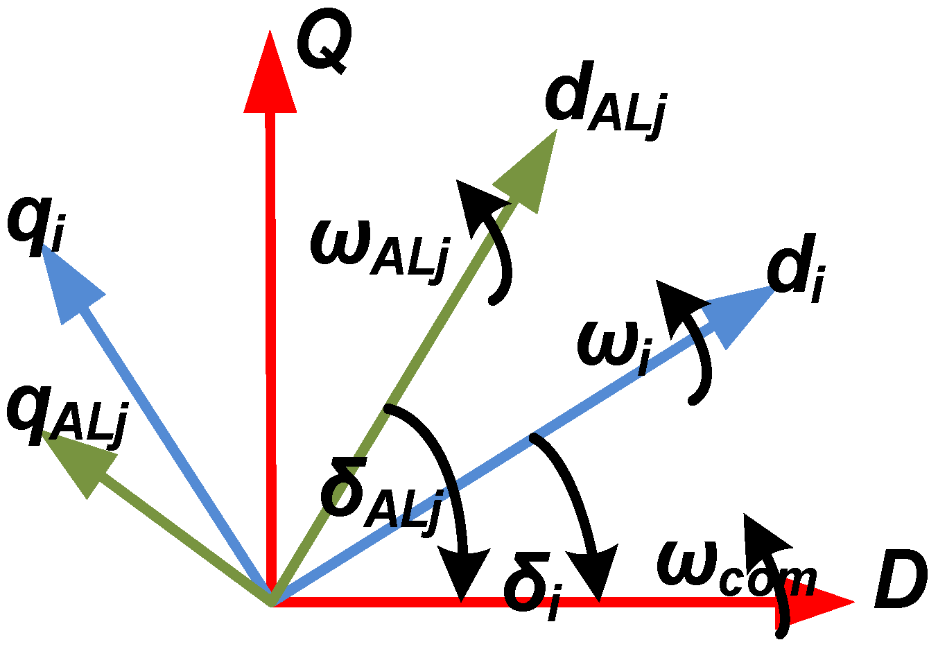
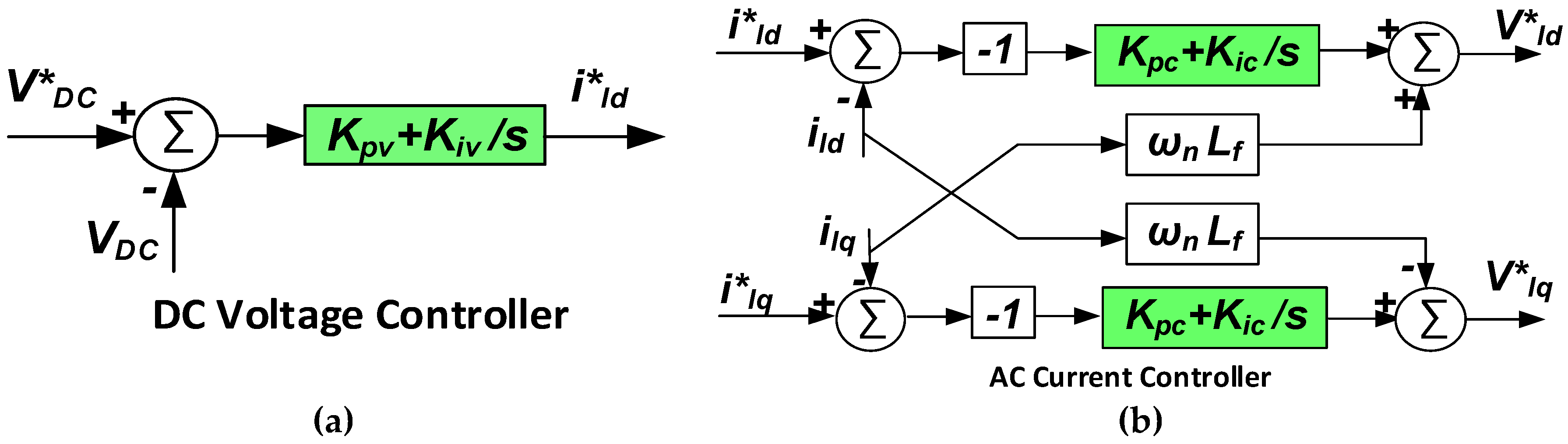
2.2. Active Load Model

Active load model with its controllers is given in Figure 1. In the following model, the active load has its own dq reference frame as each inverter has. The active load should be synchronized with the microgrid to share its angles. A traditional PLL shown in Figure 5 is used for this purpose. The input variable of the active load model is the input voltage while the output variable is the current drawn from the DG units [12]. The active load input current (i_lALDQ) is converted from the common reference frame “DQ” to the active load reference frame dq_AL using PLL.

$$\begin{array}{l}\left[i_{lALDQ}\right]=\left[T_R\right]\left[i_{lALdq}\right]\\ \left[T_R\right]=\sqrt{\frac{2}{3}}\left[\begin{array}{cc}\cos ({\delta }_i)& -\sin ({\delta }_i)\\ \sin ({\delta }_i)& \cos ({\delta }_i)\end{array}\right]\end{array}$$

(20)

where δ_i is the angle between the dq active load frame and common reference frame DQ.

To set the dq system frequency equal to the grid frequency, the regulator is arranged to maintain one component at zero by changing the frequency of dq system rotation [26]. The three-phase voltages are transformed into αβ stationary reference frame then the frequency and the inverter phase reference θ will be estimated as given in (21) & (22). The angle θ is controlled to transform from abc to dq and vice versa.

$$\omega =k_P^{PLL}(v_{oq}-v_{oq}^{\ast })+k_I^{PLL}{\displaystyle \int (v_{oq}-v_{oq}^{\ast })dt}$$

(21)

$$\theta ={\displaystyle \int (\omega -{\omega }_{ref})dt}+\theta (0)$$

(22)

where k_p^PLL and k_I^PLL are the PLL controller parameters.

As shown in Figure 6, to regulate the DC voltage and control the AC current of the active load, two PI controllers are proposed.

$$i_{ldAL}^{\ast }=K_{pv\_AL}(v_{DC}^{\ast }-v_{DC})+K_{iv\_AL}{\displaystyle \int (v_{DC}^{\ast }-v_{DC})dt}$$

(23)

Tuning these controller parameters is very important to get reasonable steady-state response. Firstly, the voltage controller can be used to get the AC reference current by minimizing the error between the measured DC voltage and the DC reference voltage. Similarly, the current controller can be used to get the AC reference voltage by minimizing the error between the measured AC current and the AC reference current. A negative sign to the inverter current should be added to the voltage controller state-space equations because the active load is receiving current from the DGs. For decoupling the inductor current in the DQ axes, feed-forward terms will be involved as shown in Figure 6. Meanwhile, the state-space equations of the DC capacitor circuit can be given.

$$\begin{array}{l}{v}_{idAL}^{\ast }={\omega }_{nAL}{L}_{fAL}{i}_{lqAL}-K_{pc\_AL}(i_{ldAL}^{\ast }-i_{ldAL})-K_{ic\_AL}{\displaystyle \int (i_{ldAL}^{\ast }-i_{ldAL})dt}\\ v_{iqAL}^{\ast }=-{\omega }_{nAL}{L}_{fAL}{i}_{ldAL}-K_{pc\_AL}(i_{lqAL}^{\ast }-i_{lqAL})-K_{ic\_AL}{\displaystyle \int (i_{lqAL}^{\ast }-i_{lqAL})dt}\end{array}$$

(24)

$$\frac{d{v}_{DC}}{dt}=\frac{1}{C_{dc}}{i}_{conv}-\frac{1}{R_{dc}{C}_{dc}}{v}_{DC}$$

(25)

where C_dc and R_dc are the dc load capacitance and resistance and i_conv is the DC current of the active load.

Considering ideal power converter, the internal power losses can be neglected. Therefore, the state-space equations of the switching bridge can be written as

$$v_{idAL}{i}_{idAL}+v_{iqAL}{i}_{iqAL}=i_{conv}{v}_{DC}$$

(26)

3. Problem Formulation

Controller gains may cause poor damped responses and even the instability of the microgrid [3]. To enhance the microgrid transient performance, the controller parameters of inverters and active load, PLL gains, and power-sharing coefficients would be tuned carefully. In this paper, an optimization technique is used to obtain the parameters affecting the microgrid stability. The design problem is expressed as

3.1. Objective Function and Problem Constraints

The optimal controller parameters and optimal power-sharing coefficients are designed based on time domain simulation. The problem constraints are the parameter bounds. Therefore, the design problem can be formulated as the following optimization problem

Minimize J

(27)

Subject to {K^min ≤ K ≤ K^max, m_p^min ≤ m_p ≤ m_p^max, and n_q^min ≤ n_q ≤ n_q^max}

(28)

$$\mathrm{where} J={\displaystyle {\int }_{t=0}^{t=t_{sim}}\left[{\left(P_m-P_{ref}\right)}^2+{\left(V_{dc}-V_{dc}^{\ast }\right)}^2\right]}tdt$$

(29)

where J is a weighted objective function, K = [k_pv, k_iv, k_pc, k_ic, k_{pv_AL}, k_{iv_AL}, k_{pc_AL}, k_{ic_AL,} k_P^PLL, k_I^PLL]^T are the controller parameters constrained as K^min ≤ K ≤ K^max, m_p and n_q are the power-sharing parameters, t is minimum settling time, P_ref is the reference active power of the DG and $V_{dc}^{\ast }$ is DC reference voltage.

In the optimization procedure, the goal is to minimize J to make sure that DG inject the required active power and make sure that the dc voltage of the active load is close to the reference dc voltage. PSO starts randomly assuming their particles (controller parameters in this work). Using these parameters, the cost function J is calculated. This cost function depends mainly on the variations of P_ref and $V_{dc}^{\ast }$ as it is mentioned in Equation (29). This step will be repeated and after each step, the cost function will be compared with the minimum calculated cost function until it arrives to the lowest cost function. The corresponding parameters to this lowest cost function will be selected to be the optimal controller parameters.

3.2. Particle Swarm Optimization

In this work, PSO is utilized to obtain the optimal parameters. In 1995, stimulated by social behavior of bird gathering or fish training, Eberhart and Kennedy developed PSO as a population based stochastic optimization method [35]. It is worth mentioning that balancing between local and global search methods can be achieved using PSO. It has different advantages over other traditional optimization techniques [3]. In a PSO algorithm, the population has n particles that represent candidate solutions. Each particle is an m-dimensional real-valued vector, where m is the number of optimized parameters. Therefore, each optimized parameter represents a dimension of the problem space. The PSO technique can be summarized as follows:

1) Initialization

Starting by time counter setting then randomly n particles and their initial velocities will be generated. The objective function of each particle will be evaluated. From the obtained objective functions, the global best function J_best will be selected as the lowest objective function. Meanwhile, its associated global best particle x_best will be selected as well. To control the impact of the previous velocity on the current velocity, the inertia weight will be initiated.

2) Time Updating

The time counter will be updated.

3) Weight Updating

The inertia weight will be updated as follows w(t) = αw(t − 1) where α is a decrement constant smaller than but close to 1;

4) Velocity Updating

At each time step, each particle velocity is modified depending mostly on its current velocity and the distances between the particle and its personal and global best positions.

$$v_{n+1}^i=w{v}_n^i+c_1{r}_1\left(p_{best}-k_n^i\right)+c_2{r}_2\left(g_{best}-k_n^i\right)$$

(30)

where r₁ and r₂ are random numbers between 0 and 1; w is the inertia weight; c₁ and c₂ are the ‘trust’ parameters; g_best is the best swarm position; and p_best is the best position for particle i.

It is worth mentioning that the second term represents the cognitive part of PSO where the particle changes its velocity based on its own thinking and memory. The third term represents the social part of PSO where the particle changes its velocity based on the social-psychological adaptation of knowledge. In previous research, a variety of inertia weight strategies were proposed and developed to improve the performance of the PSO algorithm. However, the random values for most modified PSO algorithms are always generated by uniform distribution in the range of [0, 1]. Obviously, the random values represent the weights of two distances for updating the particle velocity. If the range of random values is small, these two distances have little influence on the new particle velocity, which means that the velocity cannot be effectively increased or changed to escape from local optima. In order to improve the global optimization ability of the PSO algorithm, it is necessary to expand the range of random values [41].

5) Position updating

Based on the updated velocities, the new particle position at iteration n + 1 is given

$$k_{n+1}^i=k_n^i+v_{n+1}^i$$

(31)

where kⁱ_n+1 and vⁱ_n+1 are the particle position and its velocity vector at iteration n + 1.

6) Individual Best Updating

For each particle, the cost function J will be determined according to the updated position and then it will be compared with the previous one. If this cost function at this time is less than the previous one, it will be selected as the global best J_j^*. An individual best will be also selected as a global best.

7) Global Best Updating

From the all values of the global best J_j^*, the minimum value will be selected as follows: If J_min > J^** then update global best as X^** = X_min and J^** = J_min.

8) Stopping Criteria

PSO will stop searching if the number of iterations exceeds pre-specified number or if the number of iterations exceeds the maximum allowable iterations.

3.3. PSO Implementation

A MATLAB code is built to emulate the proposed PSO–based approach. Based on our experience, PSO performance is mainly affected by the initial inertia weight and the maximum allowable velocity. To obtain the effective values of these parameters, several runs have been done. Using uniform distribution, the random values r₁ and r₂ could be generated in the traditional PSO [41]. In addition, to get the global optima effectively and quickly without falling into the local optima, large-scale random values should be selected in the PSO algorithms. However, a range of [–1, 1] is more beneficial to improve the global searching capability in a low dimensional practical optimization problem [41]. For PSO algorithm with different types of random values, the impact of random values on the particle velocity was discoursed in details [41]. Actually, to achieve an efficient PSO performance, these parameters should be carefully selected [36]. In this work, the following PSO parameters are assumed as given:

• Population size = 20;
• Decrement constant (α) = 0.98;
• Inertia weight factor = 1;
• Acceleration constants: c₁ = c₂ = 2;
• Generation or iteration = 100.

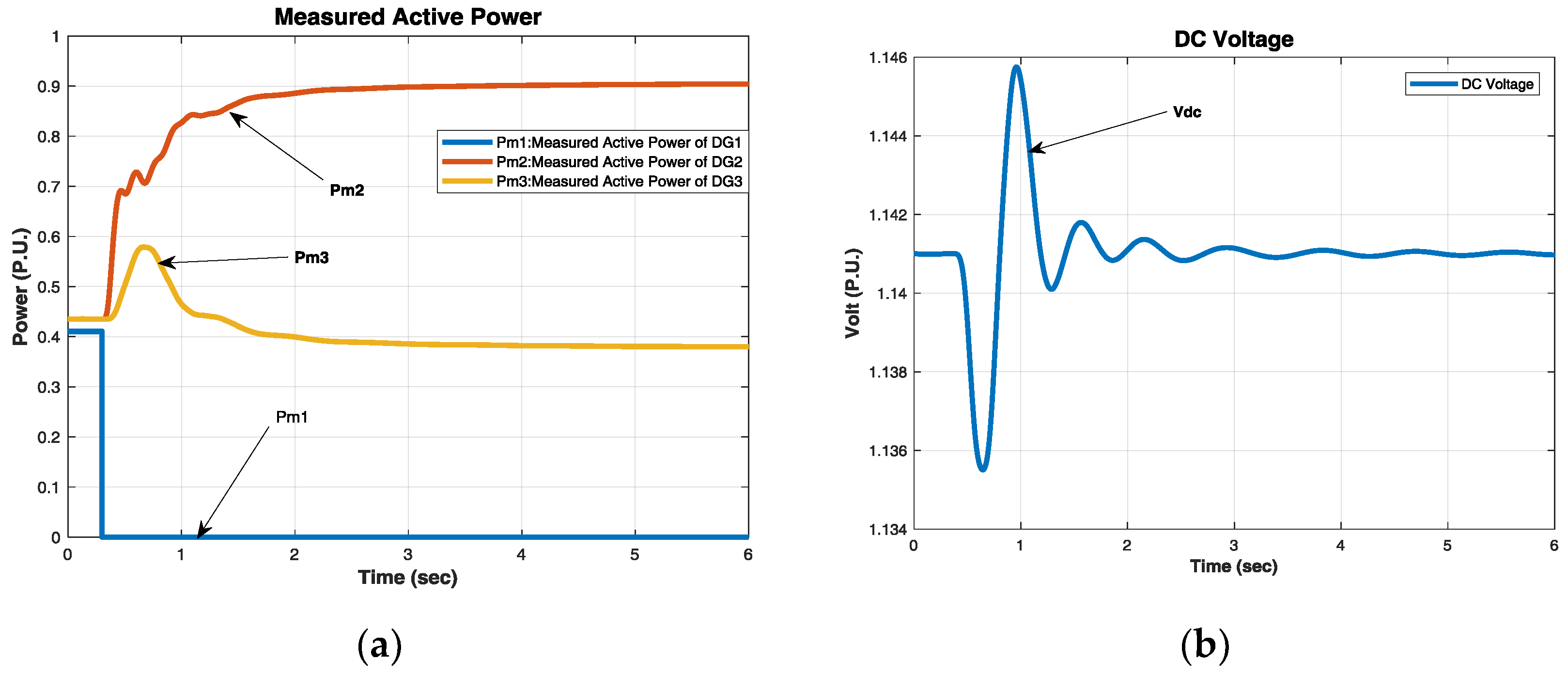
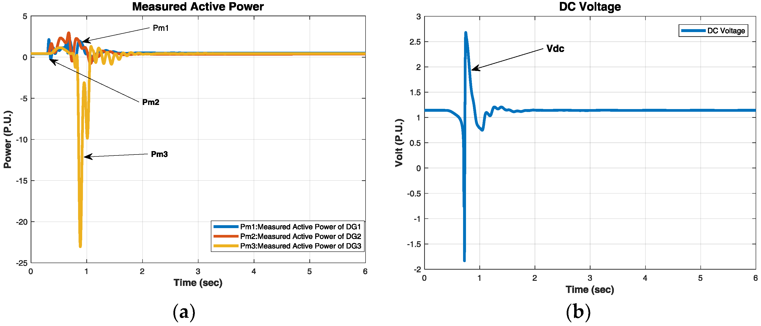
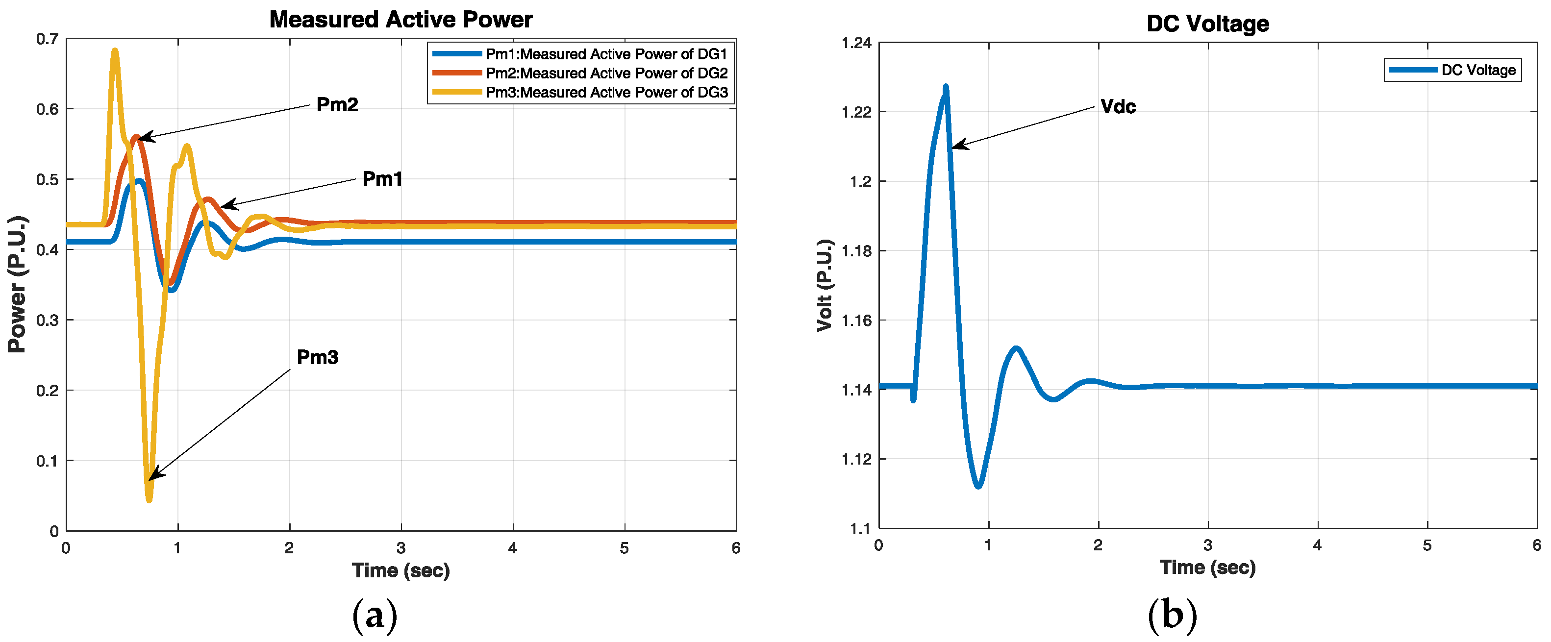
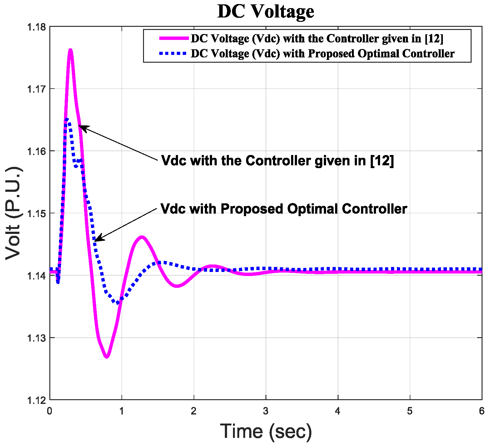
4. Results and Discussion

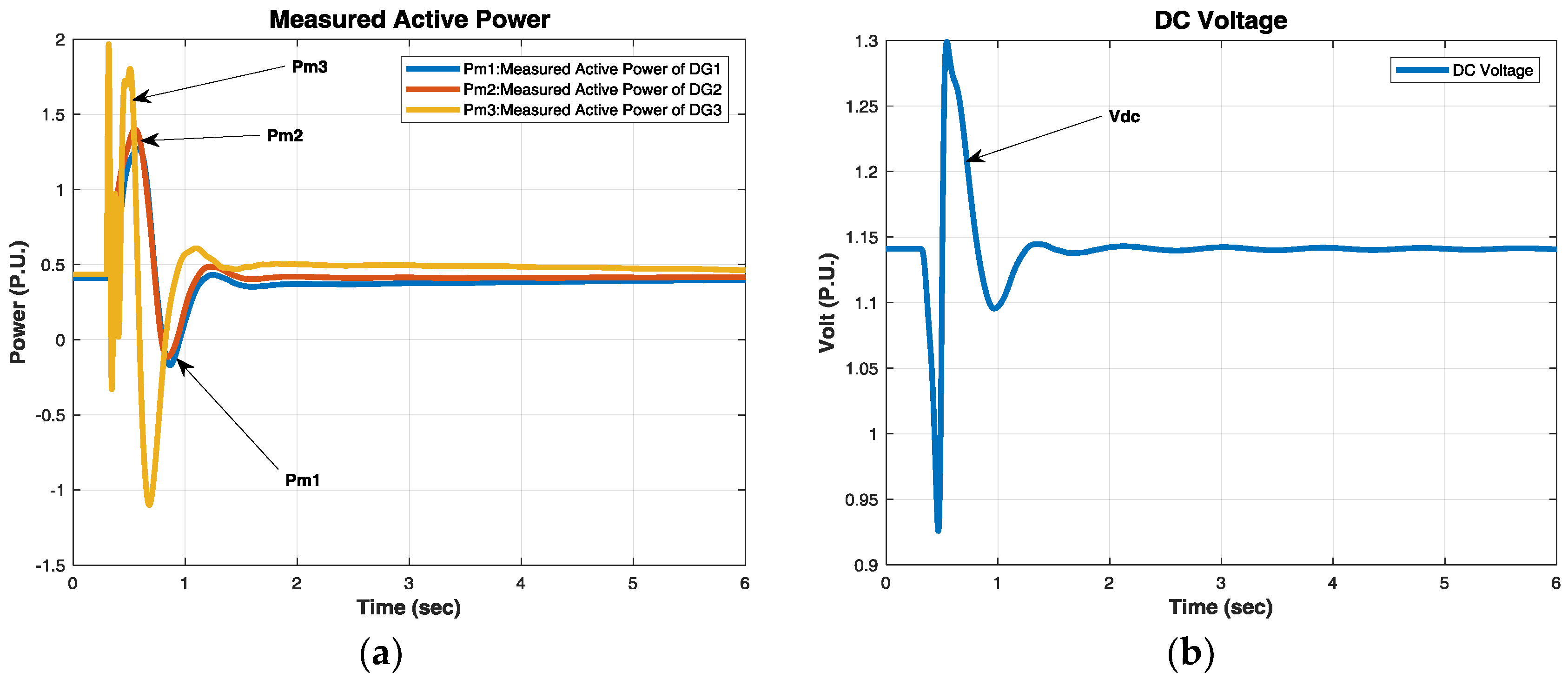
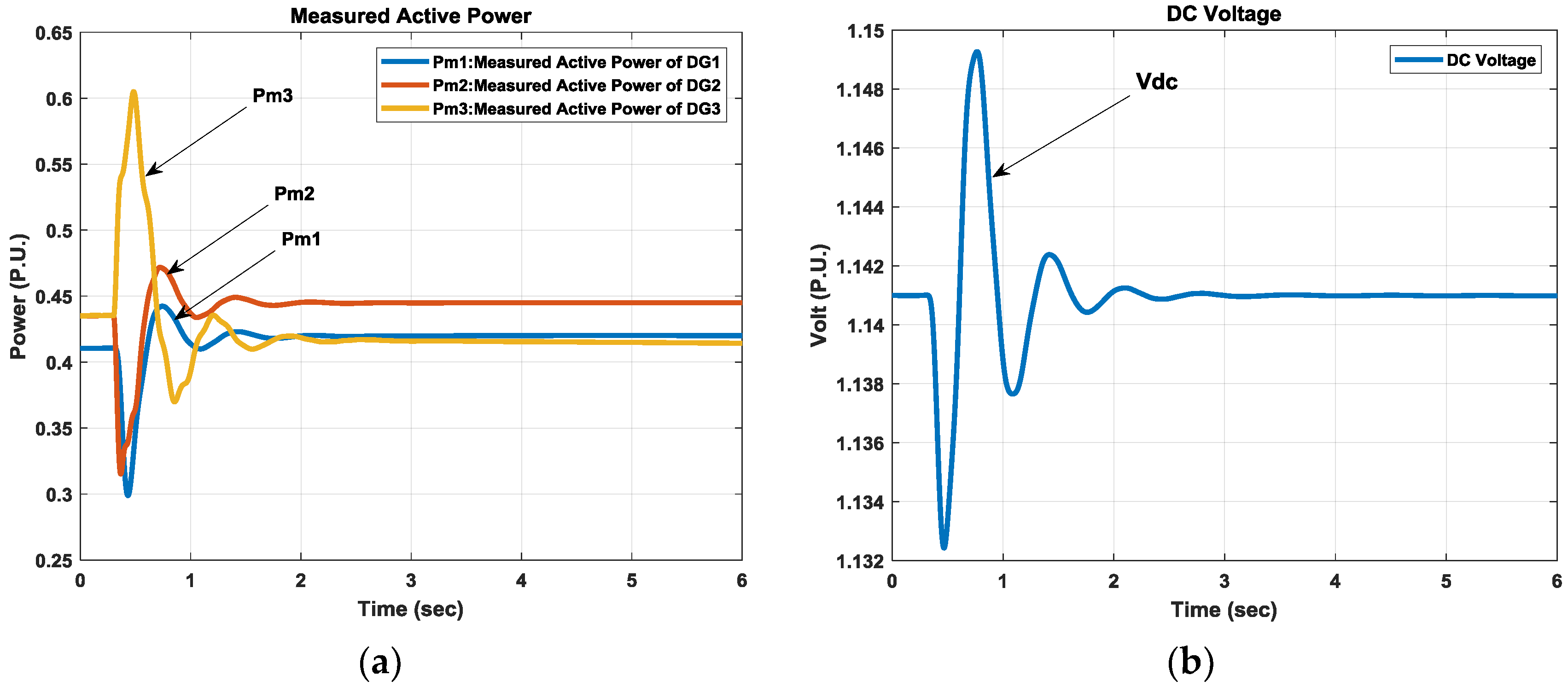
4.1. Time Domain Simulation

An autonomous microgrid shown in Figure 1 has been modeled. Three inverter-based DGs (10 kVA) are connected with CIL (5.8 kW) and CPL (7.3 kW) through coupling inductances, filters, and two transmission lines. Assuming an ideal source from the DG side, the dc bus dynamics can be neglected. With the realization of high switching frequencies (4–10 kHz), the switching process of the inverter may also be neglected [40]. The system parameters are given in

Table 1. System parameters.

Microgrid Parameters				Active Load Parameters
Parameter	Value	Parameter	Value	Parameter	Value	Parameter	Value
fs	8 kHz	Vn	381 V	Lf	2.3 mH	Lc	0.93 mH
Lf	1.35 mH	Lc	0.35 mH	Cf	8.8 × 10−6 F	rc	0.03 Ω
Cf	50 × 10−6 F	Cb	50 × 10−6 F	rf	0.1 Ω
rf	0.1 Ω	rc	0.03 Ω	Rdc	67.123 Ω	Cdc	2040 × 10−6 F
ωn	314.16 rad/s	ωc	31.416 rad/s
r1 + jx1	(0.23 + j0.1) Ω	r2 + jx2	(0.35 + j0.58) Ω

. Based on time-domain simulation, the error in the measured active power and DC voltage will be curtailed using a weighted objective function. The optimal parameters of the proposed active load and inverter controllers, PLL gains and power-sharing coefficients are presented in

Table 2. Optimal parameters.

PI Controller Parameters				Power-Sharing Parameters of the Three DG Units
Parameter	Value	Parameter	Value	Parameter	Value	Parameter	Value
kpv(Amp/Watt)	17.268074	kpc(Amp/Watt)	3.0547	mp	3.79404 × 10−7	nq	9.36593 × 10−5
	20.7258764		2.2025		6.75934 × 10−7		1.86121 × 10−5
	23.6522868		2.8311		1.71857 × 10−7		3.21349 × 10−5
kiv(Amp/Joule)	64.356192	kic(Amp/Joule)	2.4811	Active Load Parameters
	89.1177596		1.86315	kpv_AL (Amp/Watt)	4.79107648	kpc_AL (Amp/Watt)	2.3042
	−10.0262696		0.9311	kiv_AL (Amp/Joule)	62.5416616	kic_AL (Amp/Joule)	−0.3198
PLL Parameters
kPPLL	50	kIPLL	1

. Fault and step change disturbances have been applied on both ac and dc sides to explore and assess the effect of the optimal parameters on the microgrid stability. Through the time domain simulations, the microgrid performance has been examined firstly when three-phase fault occurred at active load bus. Figure 7 shows the satisfactory damping characteristics of the proposed microgrid under the fault disturbance at active load bus. Figure 7a,b depict the responses of the active power of the three DGs respectively and the DC output voltage of the DC side of the active load. To feed this fault, the output powers of the three DGs have been increased sharply after the fault immediately. Additionally, the output power of DG3 is much greater than the output powers of the DG1 & DG2 because the fault occurred at active load bus which is closed to DG3. Secondly, the microgrid performance has been examined when a three phase fault is applied at line 2 at t = 0.3 s then fault is cleared at t = 0.6 s. During this period, DG1 and DG2 respond to support the passive load by its demand while DG3 is isolated to feed the active load by its powers. Figure 8 shows the adequate damping characteristics of the proposed controller. The DGs output powers response is illustrated in Figure 8a while Figure 8b depicts the DC voltage response of the active load for this disturbance. It can be observed from the given results that the system performance has a good overshoot and settling time performance. Moreover, the results depict impressively enhanced damping characteristics. Thirdly, the controller capability is investigated and the microgrid performance is examined when the microgrid loses DG1. It means that both loads have to receive their powers from DG2 and DG3. Figure 9a,b illustrates the response of the output real power of the three DGs and the DC voltage response of the active load. Additionally, DG1 and DG2 are capable of feeding both loads after the microgrid is disturbed. After losing DG1, the results show reasonable damping characteristics of the proposed controller. From Figure 9a, at the steady state operation, the output active powers of the three DGs are 0.41, 0.43, and 0.43p.u. respectively. Therefore, the total output power is equal to 1.27p.u. While after the microgrid is cleared from the fault disturbance, the output active powers of the three DGs are 0.0, 0.37, and 0.9p.u. respectively. Therefore, the total output power is equal to 1.27p.u. This means that the total output powers of all DGs before and after fault are equal. Therefore, the two DGs (DG2 and DG3) can share the same power that the three DGs (DG1, DG2, and DG3) have shared before the microgrid lost DG1. In addition, as it was mentioned before in Section 2, each DG inverter is assumed to be connected to a constant dc power source, so there no need to regulate the dc-link voltage otherwise, a controller should be introduced to regulate the dc-link voltage [40]. Otherwise, DG3 output power could not be reached to this value since each DG source has a limited output power. For example, if DG3 represents a photovoltaic plant, the output power increase could not be available for many different reasons such as temperature and dc voltage regulations.

Fourthly, the microgrid performance has been examined when the CPL voltage stepped down to 0.5p.u. The DGs output power and active load DC voltage responses are provided in Figure 10a,b. It can be observed from the given results that the system performance has a good overshoot and settling time performance. Furthermore, the results depict impressively enhanced damping characteristics. Figure 10 shows reasonable damping characteristics of the proposed controller. It is worth mentioning that if the microgrid has a protection system, the protection system should respond very quickly for such a big disturbance. However, the main goal of this study is to check the effectiveness of the proposed controller for such disturbance like this. Fifthly, to guarantee the controller capability, another disturbance has been applied at dc side of the active load. Through the time domain simulation, the proposed controller has been explored when the DC reference voltage stepped up by 5%. Figure 11a,b show the DGs output power response and the DC voltage response of the active load respectively. To demonstrate its superiority, the proposed optimal controller is finally compared with the controller presented in [12]. The DC voltage response of the active load in both cases when a three-phase fault occurred at CPL bus is shown in Figure 12. The optimal parameters of are used to show the priority of the proposed case. From the controller results shown, the proposed controller has improved dynamic performance after getting disturbed.

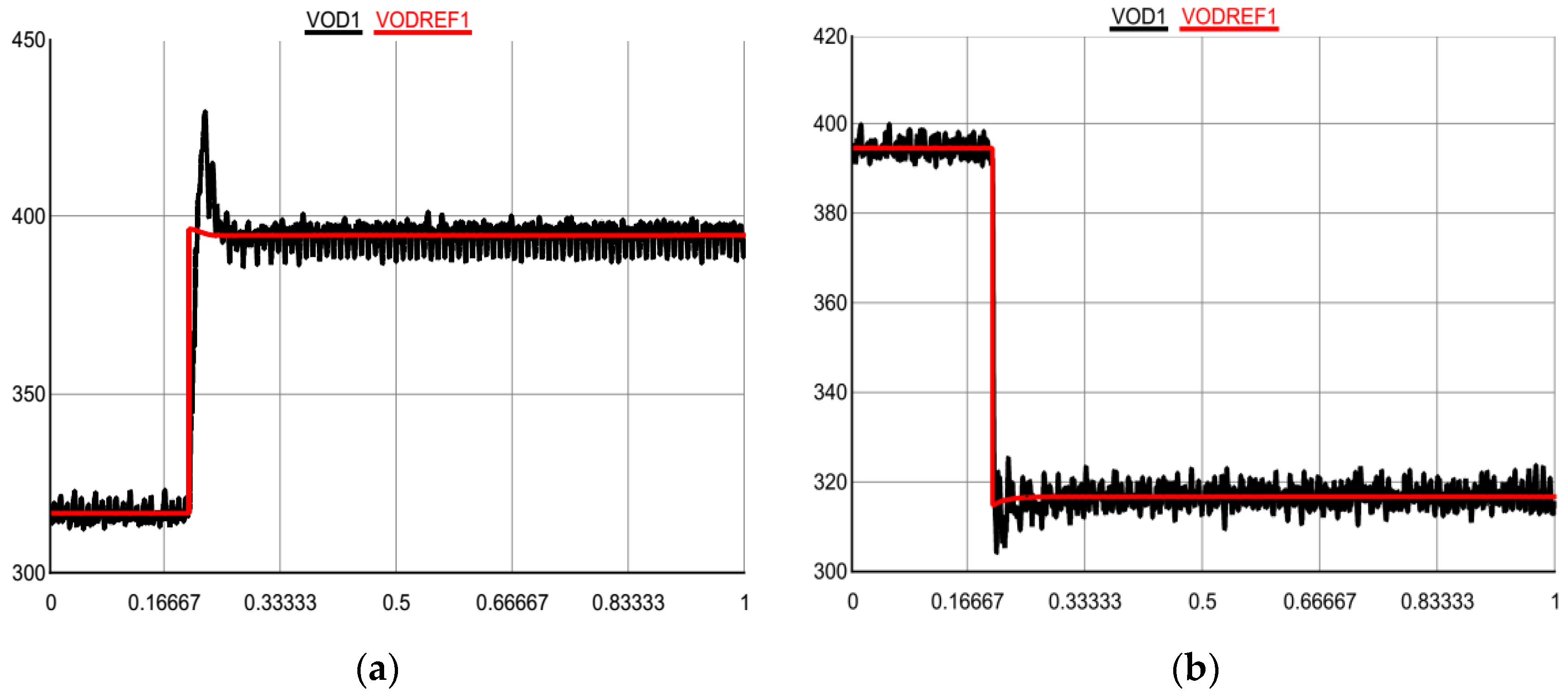
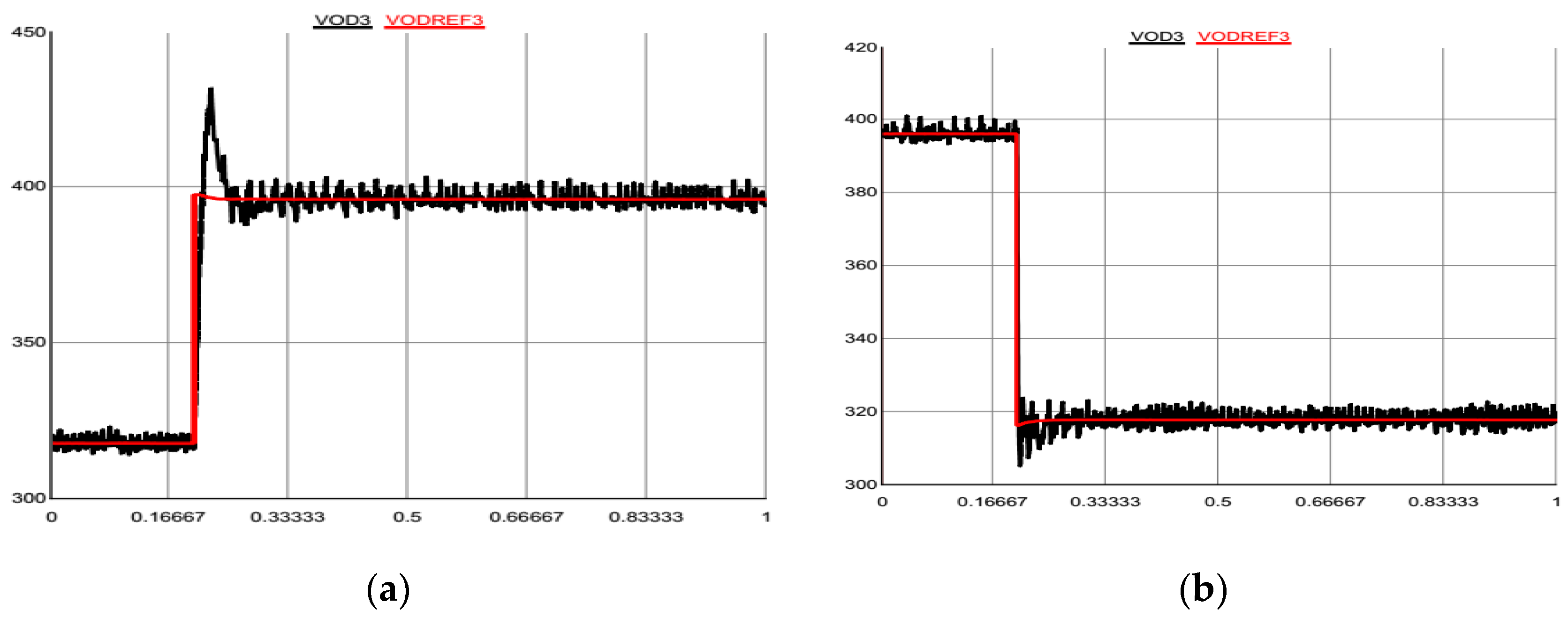
4.2. Experimental Implementation and Results

Recently, it has been made possible to simulate electrical networks using real-time digital simulator (RTDS) to verify the theoretical simulation [38,39]. The simulation could be performed faster in RTDS since it works continuously in sustained real-time. Microgrid elements such as loads, converter bridges, filters, and lines can be modeled inside the RTDS environmental using their physical representation built in a standard library blocks. Additionally, each power system component has its detailed model, which is already built in RTDS library. This model can resemble the real system. The converter (inverter/rectifier) bridge is ideally modeled. The inverters controllers and active load controllers are implemented in the RTDS using the optimal parameters obtained from PSO. The performance of the proposed controllers has been comprehensively tested. RTDS is used to analyze the microgrid described previously in Section 2. The microgrid setup including the inverter-based DGs and active load circuits is simulated using the RTDS. In real time, the controller performance of the autonomous microgrid is assessed using the optimal controller parameters. The effectiveness of the proposed approach for stability enhancement is investigated. With step up and down changes of the DG1 reference voltage, Figure 13a,b shows the DG1 output voltage and its reference respectively. The results show the controller effectiveness under the sever disturbances. Similarly, step up and down changes for the reference voltage of DG3 is applied to investigate the controller effectiveness. Figure 14a,b depict the output voltage of the DG3 and its reference due to this change. As shown in the RTDS results, the capability of the controller to track the reference during the step change is satisfactory without significant overshoot and delay time.

5. Conclusions

In this paper, an autonomous microgrid including active load has been modeled and analyzed. The stability of the inverter-based microgrids considering active load has been assessed. By minimizing the proposed objective function using particle swarm optimization, the control problem has been optimally designed. A weighted objective function has been used to curtail the errors in the measured active power and DC voltage based on time-domain simulations. Different AC and DC disturbances have been introduced to verify the optimal parameters effect on the microgrid stability. The proposed controllers successfully coordinate among the distributed energy resources. Results show satisfactory performance with efficient damping characteristics of the considered autonomous microgrid. Additionally, results prove the superiority of the proposed optimal controller over the controller presented in the literature. The considered microgrid including the three DGs, active loads, and their associated controllers has been developed and implemented on real time digital simulator (RTDS). The performance of three inverter-based DGs as well as the active load of the considered autonomous microgrid with the proposed controllers has been verified on RTDS. The experimental results confirm the effectiveness of the proposed controllers to enhance the stability of the proposed microgrid under different disturbances and operating conditions.

References

1. Colmenar-Santos, A.; Reino-Rio, C.; Borge-Diez, D.; Collado-Fernández, E. Distributed generation: A review of factors that can contribute most to achieve a scenario of DG units embedded in the new distribution networks. Renew. Sustain. Energy Rev. 2016, 59, 1130–1148. [Google Scholar] [CrossRef]
2. Hatziargyriou, N. Microgrids: Architectures and Control; John Wiley & Sons: Chichester, UK, 2013. [Google Scholar]
3. Hassan, M.; Abido, M. Optimal design of microgrids in autonomous and grid-connected modes using particle swarm optimization. IEEE Trans. Power Electron. 2011, 26, 755–769. [Google Scholar] [CrossRef]
4. Raju, E.; Jain, T. Robust optimal centralized controller to mitigate the small signal instability in an islanded inverter based microgrid with active and passive loads. Electr. Power Energy Syst. 2017, 90, 225–236. [Google Scholar] [CrossRef]
5. Han, H.; Hou, X.; Yang, J.; Wu, J.; Su, M.; Guerrero, J.M. Review of power sharing control strategies for islanding operation of ac microgrids. IEEE Trans. Smart Grid 2016, 7, 200–215. [Google Scholar] [CrossRef]
6. Chandorkar, M.; Divan, D.; Adapa, R. Control of parallel-connected inverters in standalone ac supply systems. IEEE Trans. Ind. Appl. 1993, 29, 136–143. [Google Scholar] [CrossRef]
7. Olivares, D.; Mehrizi-Sani, A.; Etemadi, A.H.; Cañizares, C.A.; Iravani, R.; Kazerani, M.; Hajimiragha, A.H.; Gomis-Bellmunt, O.; Saeedifard, M.; Palma-Behnke, R.; et al. Trends in microgrid control. IEEE Trans. Smart Grid 2014, 5, 1905–1919. [Google Scholar] [CrossRef]
8. Tsikalakis, A.; Hatziargyriou, N. Centralized control for optimizing microgrids operation. In Proceedings of the IEEE Power and Energy Society General Meeting, San Diego, CA, USA, 24–29 July 2011. [Google Scholar]
9. Tan, K.; Peng, X.; So, P.; Chu, Y.; Chen, M. Centralized control for parallel operation of distributed generation inverters in microgrids. IEEE Trans. Smart Grid 2012, 3, 1977–1987. [Google Scholar] [CrossRef] [Green Version]
10. Liang, H.; Choi, B.J.; Zhuang, W.; Shen, X. Stability enhancement of decentralized inverter control through wireless communications in microgrids. IEEE Trans. Smart Grid 2013, 4, 321–331. [Google Scholar] [CrossRef]
11. Wang, Y.; Wang, X.; Chen, Z.; Blaabjerg, F. Distributed optimal control of reactive power and voltage in islanded microgrids. IEEE Trans. Ind. Appl. 2017, 53, 340–349. [Google Scholar] [CrossRef]
12. Bottrell, N.; Prodanovic, M.; Green, T. Dynamic stability of a microgrid with an active load. IEEE Trans. Power Electron. 2013, 28, 5107–5119. [Google Scholar] [CrossRef]
13. He, J.; Li, Y. An enhanced microgrid load demand sharing strategy. IEEE Trans. Power Electron. 2017, 27, 3984–3995. [Google Scholar] [CrossRef]
14. Guerrero, J.; Loh, P.; Chandorkar, M. Advanced control architectures for intelligent microgrids—Part I: Decentralized and hierarchical control. IEEE Trans. Ind. Electron. 2013, 60, 1254–1262. [Google Scholar] [CrossRef]
15. He, J.; Li, Y.; Guerrero, J. An islanding microgrid power sharing approach using enhanced virtual impedance control scheme. IEEE Trans. Power Electron. 2013, 28, 5272–5282. [Google Scholar] [CrossRef]
16. Zhong, Q. Robust droop controller for accurate proportional load sharing among inverters operated in parallel. IEEE Trans. Ind. Electron. 2013, 60, 1281–1290. [Google Scholar] [CrossRef]
17. Lee, C.; Chu, C.; Cheng, P. A new droop control method for the autonomous operation of distributed energy resource interface converters. IEEE Trans. Power Electron. 2013, 28, 1980–1993. [Google Scholar] [CrossRef]
18. Perreault, D.; Selders, R., Jr.; Kassakian, J. Frequency based current-sharing techniques for paralleled power converters. IEEE Trans. Power Electron. 1988, 13, 626–634. [Google Scholar] [CrossRef]
19. Tuladhar, A.; Jin, H.; Unger, T. Control of parallel inverters in distributed AC power systems with consideration of line impedance effect. IEEE Trans. Ind. Appl. 2000, 36, 131–138. [Google Scholar] [CrossRef]
20. Han, Y.; Li, H.; Shen, P.; Coelho, E.; Guerrero, J. Review of active and reactive power sharing strategies in hierarchical controlled microgrids. IEEE Trans. Power Electron. 2017, 32, 2427–2451. [Google Scholar] [CrossRef]
21. Emadi, A.; Khaligh, A.; Rivetta, C.; Williamson, G. Constant power loads and negative impedance instability in automotive systems: Definition, modeling, stability, and control of power electronic converters and motor drives. IEEE Trans. Veh. Technol. 2006, 55, 1112–1125. [Google Scholar] [CrossRef]
22. Sanchez, S.; Ortega, R.; Grino, R.; Bergna, G.; Molinas, M. Conditions for existence of equilibria of systems with constant power loads. IEEE Trans. Circuits Syst. I Regul. Pap. 2014, 61, 2204–2211. [Google Scholar] [CrossRef]
23. Hassan, M. Dynamic Stability of an Autonomous Microgrid Considering Active Load Impact with New Dedicated Synchronization Scheme. IEEE Trans. Power Syst. 2018, 1–12. [Google Scholar] [CrossRef]
24. Dong, D.; Wen, B.; Boroyevich, D.; Mattavelli, P.; Xue, Y. Analysis of phase-locked loop low-frequency stability in three-phase grid-connected power converters considering impedance interactions. IEEE Trans. Ind. Electron. 2015, 62, 310–321. [Google Scholar] [CrossRef]
25. Svensson, J. Synchronization methods for grid-connected voltage source converters. IEE Proc. Gener. Transm. Distrib. 2001, 148, 229–235. [Google Scholar] [CrossRef]
26. Chen, J.; Chen, J. Stability analysis and parameters optimization of islanded microgrid with both ideal and dynamic constant power loads. IEEE Trans. Ind. Electron. 2018, 65, 3263–3274. [Google Scholar] [CrossRef]
27. Mahmoudi, A.; Hosseinian, S.; Kosari, M.; Zarabadipour, H. A new linear model for active loads in islanded inverter-based microgrid. Int. J. Electr. Power Energy Syst. 2016, 81, 104–113. [Google Scholar] [CrossRef]
28. Magne, P.; Nahid-Mobarakeh, B.; Pierfederci, S. Dynamic consideration of dc microgrids with constant power loads and active damping system; a design method for fault-tolerant stabilizing system. IEEE J. Emerg. Sel. Top. Power Electron. 2014, 2, 562–570. [Google Scholar] [CrossRef]
29. Marx, D.; Magne, P.; Nahid-Mobarakeh, B.; Pierfederici, S.; Davat, B. Large signal stability analysis tools in dc power systems with constant power loads and variable power loads—A review. IEEE Trans. Power Electron. 2012, 27, 1773–1787. [Google Scholar] [CrossRef]
30. Du, W.; Zhang, J.; Zhang, Y.; Qian, Z. Stability criterion for cascaded system with constant power load. IEEE Trans. Power Electron. 2013, 28, 1843–1851. [Google Scholar] [CrossRef]
31. Karimipour, D.; Salmasi, F. Stability Analysis of AC Microgrids with Constant Power Loads Based on Popov’s Absolute Stability Criterion. IEEE Trans. Circuits Syst. II 2015, 62, 696–700. [Google Scholar] [CrossRef]
32. Guo, X.; Lu, Z.; Wang, B.; Sun, X.; Wang, L.; Guerrero, J. Dynamic phasors-based modeling and stability analysis of droop-controlled inverters for microgrid applications. IEEE Trans. Smart Grid 2014, 5, 2980–2987. [Google Scholar] [CrossRef]
33. Khorramabadi, S.; Bakhshai, A. Critic-based self-tuning PI structure for active and reactive power control of VSCs in microgrid systems. IEEE Trans. Smart Grid 2015, 6, 92–103. [Google Scholar] [CrossRef]
34. Moafi, M.; Marzband, M.; Savaghebi, M.; Guerrero, J. Energy management system based on fuzzy fractional order PID controller for transient stability improvement in microgrids with energy storage. Int. Trans. Electr. Energy Syst. 2016, 26, 2087–2106. [Google Scholar] [CrossRef]
35. Kennedy, J.; Eberhart, R. Particle swarm optimization. In Proceedings of the IEEE International Conference on Neural Networks, Perth, Western Australia, 27 November–1 December 1995; Volume 4, pp. 1942–1948. [Google Scholar]
36. Abido, M. Optimal design of power-system stabilizers using particle swarm optimization. IEEE Trans. Energy Convers. 2002, 17, 406–413. [Google Scholar] [CrossRef]
37. Real Time Digital Simulator Power System and Control User Manual; RTDS Technologies: Winnipeg, MB, Canada, 2009.
38. Forsyth, P.; Kuffel, R. Utility applications of a RTDS simulator. In Proceedings of the IPEC International Power Engineering Conference, Singapore, 3–6 December 2007; pp. 112–117. [Google Scholar]
39. Li, Y.; Vilathgamuwa, D.; Loh, P. Design, analysis, and real-time testing of a controller for multibus microgrid system. IEEE Trans. Power Electron. 2004, 19, 1195–1204. [Google Scholar] [CrossRef]
40. Hornik, T.; Zhong, Q. A Current-Control Strategy for Voltage-Source Inverters in Microgrids Based on H∞ and Repetitive Control. IEEE Trans. Power Electron. 2011, 26, 943–952. [Google Scholar] [CrossRef]
41. Dai, H.-P.; Chen, D.-D.; Zheng, Z.-S. Effects of Random Values for Particle Swarm Optimization Algorithm. Algorithms 2018, 11, 23. [Google Scholar] [CrossRef]
Figure 1. Microgrid with active load.
Energies 11 01109 g001
Figure 2. Power droop controller.
Energies 11 01109 g002
Figure 3. Voltage and current controllers.
Energies 11 01109 g003
Figure 4. Common reference frame (DQ).
Energies 11 01109 g004
Figure 5. Phase locked loop (PLL).
Energies 11 01109 g005
Figure 6. Active load controllers.
Energies 11 01109 g006
Figure 7. Microgrid response when a three-phase fault occurred at CPL bus.
Energies 11 01109 g007
Figure 8. Microgrid response when a three-phase fault occurred at line 2.
Energies 11 01109 g008
Figure 9. Microgrid response when the microgrid loses DG1.
Energies 11 01109 g009
Figure 10. Microgrid response when active load voltage stepped down to 0.5pu.
Energies 11 01109 g010
Figure 11. Microgrid response when the reference dc voltage stepped up by 5%.
Energies 11 01109 g011
Figure 12. Comparison of DC voltage responses of the active load when a fault occurred at CPL bus.
Energies 11 01109 g012
Figure 13. (a) DG1 output voltage and (b) DG1 reference voltage due to voltage step changes.
Energies 11 01109 g013
Figure 14. (a) DG3 output voltage and (b) DG3 reference voltage due to voltage step changes.
Energies 11 01109 g014