Wide-Area Measurement—Based Model-Free Approach for Online Power System Transient Stability Assessment

Abstract

Online assessment of transient stability of power systems is critical for avoiding blackout. The increasing installation of phasor measurement units in power systems and the advancement of the wide-area measurement systems make it possible to develop methods for online assessment of power systems by using a large amount of real-time synchronous data. In this paper, we propose an approach based on the largest Lyapunov exponent (LLE) for online transient rotor angle stability assessment, using only wide-area measurement systems data. Through establishing a mathematical model that accounts for the LLE value and the rotor speed, as well as analyzing the post-fault phase-plane trajectory, we present a fast stability criterion to determine whether transient instability occurs. The proposed approach is model-free and does not need long-time LLE data to identify the final sign of the LLE. Furthermore, to reduce computational cost and realize online assessment for large-scale power systems, the critical generator pair (CGP) is recognized as the observation for the rotor angle stability assessment, and an effective algorithm for identifying the CGP is presented. Several case studies on the IEEE-39 bus test system and East China power grid are reported to demonstrate the accuracy and effectiveness of the proposed approach.

1. Introduction

Transient rotor angle stability is defined as the ability of synchronous generators of a power system to remain in synchronism after being subjected to a disturbance [1]. Since the advancement of wide-area measurement system (WAMS) based on synchronized phasor measurements has made it possible to gain real-time information of transient stability status in power systems [2], power system transient stability assessment and emergency control have received renewed interests [3,4,5]. However, online transient rotor angle stability assessment is confronted with some serious challenges due to the increasing scale and more complex dynamics of power systems.

Presently available methods for real-time transient rotor angle stability assessment after a fault are mostly classified into two categories: model-based methods [6,7] and model-free methods [8,9]. Model-based methods that depend on a power system model are not particularly appropriate for online stability assessment implementation due to computational complexity and high computation cost associated with the size of power system [10,11,12]. Model-free methods, which are independent of any system model or parameter, can avoid incorrect assessment results caused by model parameter errors. As a typical model-free method, machine learning (ML) has gained interest among power system researchers. ML methods mainly include decision tree (DT), artificial neural network (ANN), support vector machine (SVM), and so on. In [13], an approach for out-of-step prediction of synchronous generators was presented based on DT theory, and the measurements data were used for DT induction and deduction. An approach for predicting the generator rotor angle using ANN for power system stability was presented in [14], where the stability status of each generator was predicted. In [15], a hierarchical scheme for transient stability prediction based on SVM ensemble classifier was proposed. Reference [16] employed recurrent neural network (RNN) and long short-term memory (LSTM) for online transient stability assessment by using phasor measurement unit (PMU) measurements. A confidence index of the SVM-based classifier was defined to evaluate the transient stability prediction results. In [17], an ML approach based on an ensemble of online sequential extreme learning machines (EOS-ELM) with binary Jaya-based feature selection was proposed with consideration of post-fault dynamic-state information. The above methods generate a database as the input of a given network considering possible conditions, and the classifiers are trained by applying these methods to assess the power system stability. However, two limitations of ML methods are that (1) the classifiers depend entirely on the network configuration and (2) the generated database needs a large number of samples obtained offline.

To circumvent the above problems involved in using model-based methods and ML methods, this paper proposes a model-free rotor angle stability assessment method based on the largest Lyapunov exponent (LLE). Lyapunov exponents (LEs)—which characterize the separation rate of nearby trajectories in the state space and the sensitivity of a dynamical system to its initial condition—are important indices for quantifying the stability of system [18]. The LLE of a dynamical system can be used to examine whether the system reaches the stable steady-state equilibrium point or not [19]. Several LLE-based methods for analyzing rotor angle stability of the post-fault power systems were proposed in [20,21,22]. Reference [20] proposed an online monitoring algorithm based on PMU for rotor angle stability of power systems, where LLE is used to identify the out-of-step behavior of the power system after a fault. Reference [21] conducted a systematic stability analysis of a power system by using the concept of LEs, in which stability region and critical clearing time are determined by the LEs. It was found that the LLE value under a specific fault condition is invariant of the fault-clearing time up to the critical clearing time. However, the algorithms for calculating the LLE in [20,21] are model-based, so they are computationally expensive for large-scale power systems. Therefore, Dasgupta proposed a model-free LLE calculation approach for transient rotor angle stability monitoring [22] and real-time short-term voltage stability monitoring [23], in which the LLE is estimated by only using PMU measurements.

The model-free LLE estimation algorithm in [22] is a simple method with small computation cost, and only requires rotor angle measurements. Thus, it can not only eliminate the model errors, but also can be appropriate for online application. However, the time window, which is crucial for achieving reliable, accurate, and timely stability assessment results, must be prespecified when applying the algorithm for monitoring the system stability. The optimal window size is difficult to be predetermined because the optimal window size depends on fault scenarios. Furthermore, the LLE estimated by the algorithm may fluctuate between negative and positive values for quite a long time. Therefore, the rotor angle stability monitoring approach in [22] cannot be used for rapid transient stability assessment.

In this paper, a novel approach is proposed for assessing transient rotor angle stability by combining the LLE–time curve obtained by the model-free algorithm with the dynamic features of the post-fault phase-plane trajectory. To rapidly identify whether a disturbance will lead to transient instability, a new stability criterion is presented that combines the LLE with the relative rotor speed of the generator pair (GP). The proposed approach is purely data-driven and does not require any models or parameters of systems. Compared with the existing LLE-based approaches, the proposed approach does not need a large time calculation for the LLE–time curves to monitor the final signs of the LLEs, and the sampling rate has no great effect on stability assessment results. Most importantly, the proposed approach can always make a reliable and fast identification from the crucial features of the rotor speed and the corresponding LLE curves.

The remainder of this paper is organized as follows. Section 2 describes the transient rotor angle stability conditions by analyzing the dynamic features of the phase-plane trajectories. Section 3 provides the stability criterion and the scheme for online rotor angles stability assessment. In Section 4, simulation results on IEEE-39 test system and East China Power Grid (ECG) are presented. Section 5 discusses two key computational aspects and the differences between the approach proposed in this paper and the approach in [22]. Section 6 draws the conclusions.

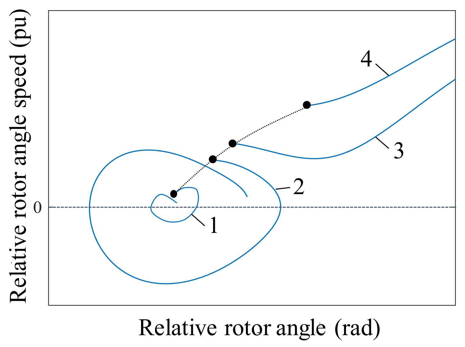
2. Transient Rotor Angle Stability Analysis Based on Post-Fault Phase-Plane Trajectories

From a system-theoretic viewpoint, the transient rotor angle stability is defined as follows [1]:

Definition 1.

The system shows asymptotic angle stability if for all i, j, there is a $k_{ij}<\infty$ such that:

$${\lim }_{t\to \infty }\left|{\theta }_i(t)-{\theta }_j(t)\right|=k_{ij}$$

(1)

According to Definition 1, it can be known that the system is rotor angle stable if the relative angle differences between all possible pairs of generators tend to be constant. Considering a multi-machine power system in which the number of the generators is n, the dynamics of each machine can be described as Equation (2).

$$\{\begin{array}{l}{\dot{\delta }}_i={\omega }_0\Delta {\omega }_i\\ \Delta {\dot{\omega }}_i=\frac{1}{M_i}(P_{mi}-P_{ei})\end{array},i=1,2\cdots ,n$$

(2)

where δ_i is the rotor angle of generator i; Δω_i is the rotor angle speed with respect to a synchronous frame of the generator i; M_i is the inertia constant of generator i; P_mi and P_ei are the mechanical power input and electric power output of generator i. Taking a GP of generators i and j as an example to analyze the transient rotor angle stability of a GP, the following is a discussion of the dynamic features of the post-fault phase-plane trajectories. Figure 1 depicts the typical dynamic features of the phase-plane trajectories of the GP after clearing fault with different fault-clearing times. (The black spots in Figure 1 denote the points of the phase-plane trajectories at the fault-clearing time.)

Stability Condition 1: In this condition, the fault is removed as soon as it occurs, and the GP shows rotor angle stability. Corresponding to Curve 1 in Figure 1, the relative rotor angle δ_ij gradually tends to be a stable value after a period of oscillation, and the relative rotor speed Δω_ij increases with a decreasing rate and then tends to be zero after a period of oscillation.

Stability Condition 2: In this condition, the GP finally tends to be rotor angle stable. Corresponding to Curve 2 in Figure 1, δ_ij oscillates and then tends to be stable, while Δω_ij decreases, then oscillates, and finally tends to be zero.

Stability Condition 3: In this condition, the GP shows rotor angle instability. Corresponding to Curve 3 in Figure 1, δ_ij keeps increasing, and Δω_ij decreases for a short time and then keeps increasing quickly.

Stability Condition 4: In this condition, the GP shows rotor angle instability due to the long duration of fault. Corresponding to Curve 4 in Figure 1, δ_ij keeps increasing and Δω_ij accelerates.

3. Online Rotor Angle Stability Assessment Scheme

3.1. LLE Calculation from Time Series

In the ergodic theory of dynamical systems, the LEs can be considered to reflect the exponential divergence or convergence of nearby trajectories in the state space of the dynamic system [24]. The LLE of a dynamical system is used as the stability certificate. The positive (negative) value of the LLE indicates that the nearby trajectories diverge (converge) and hence the system is unstable (asymptotically stable). Several algorithms using time-series data for computing the LLE have been proposed [20,21,22,23]. In this paper, the model-free algorithm presented in [22] is applied for online computation of the LLE of the relative rotor angle, and the algorithm based on the rotor angle samples from WAMS is summarized below:

(1)

Get the rotor angle time series data of the generators from WAMS. Suppose that n is the number of generators in the power grid, and θ_i(t) is a rotor angle vector of the generator i (i = 1, 2, 3, …, n) valued time series data for t = 0, ∆t, 2∆t, …, N∆t, where ∆t is the sampling period. Take one of the rotor angles denoted by θ_R(t) as the reference and define the relative rotor angle with respect to ${\mathsf{\theta }}_{\mathrm{R}}\left(\mathrm{t}\right)$ as:${\delta }_i\left(t\right)={\theta }_i\left(t\right)-{\theta }_R\left(t\right)$, i ≠ R.

(2)

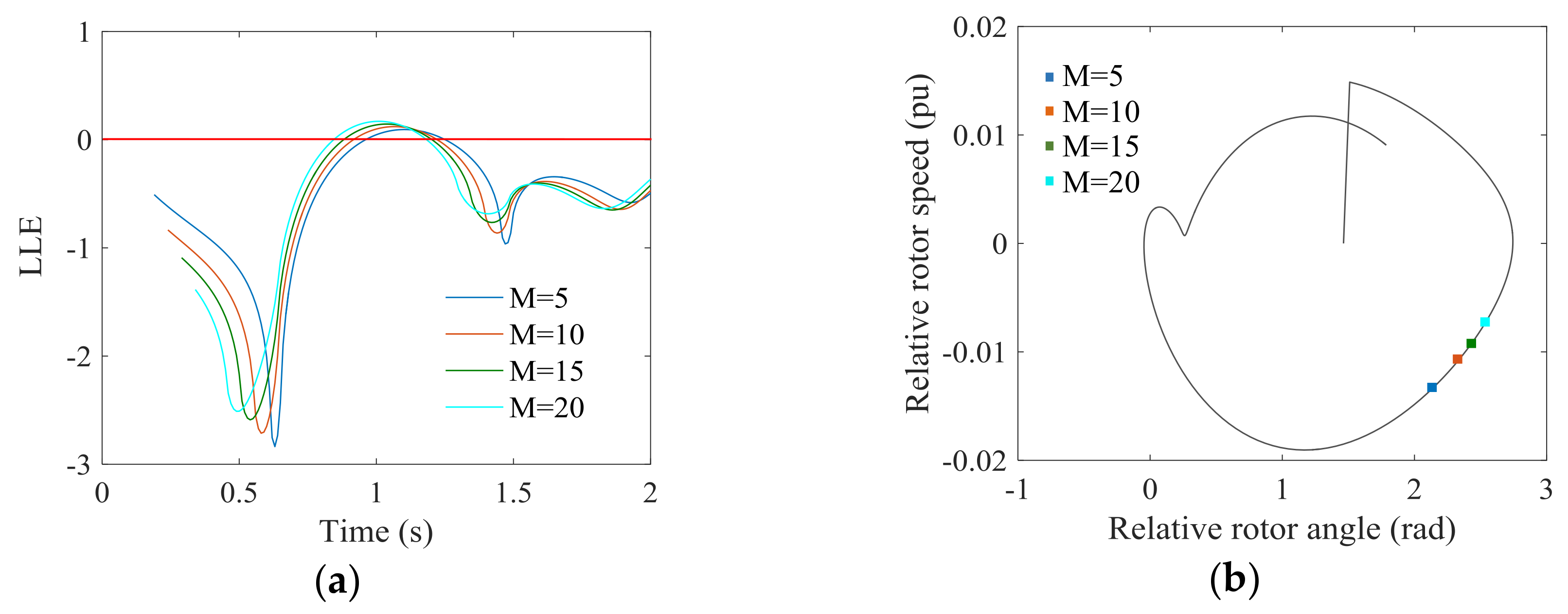
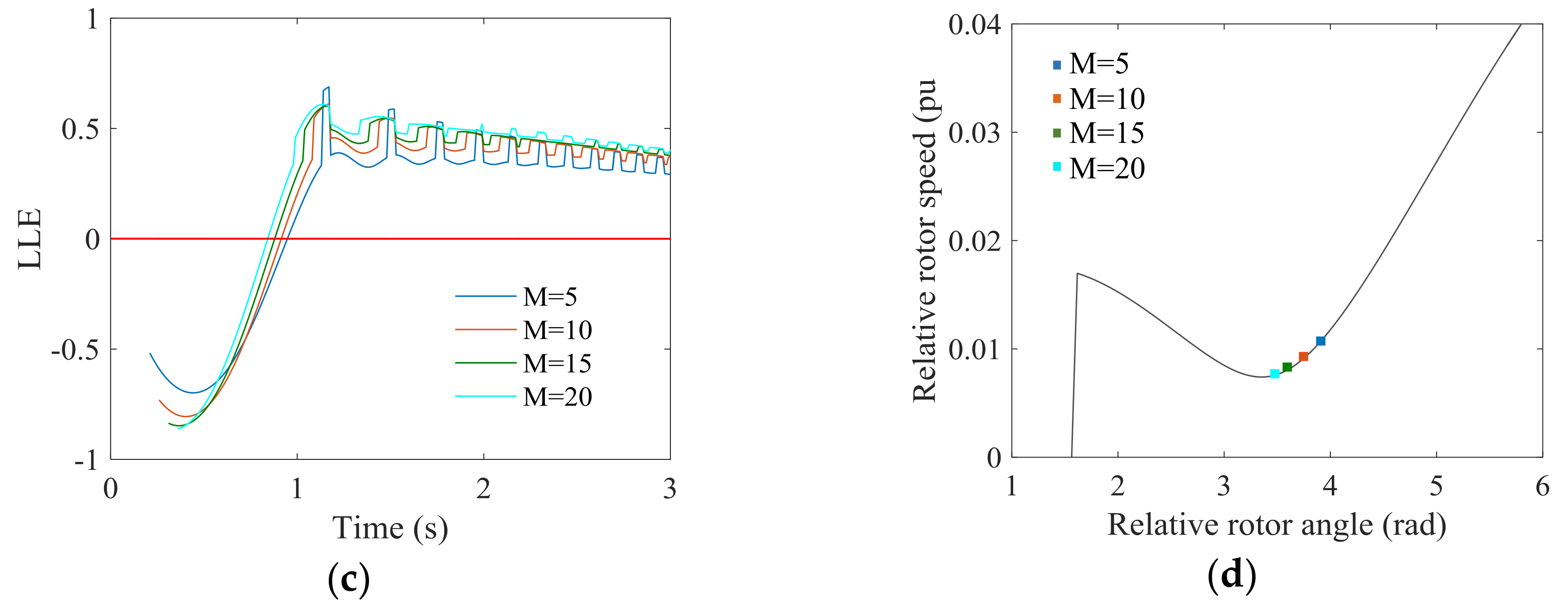
Choose M initial conditions, and calculate the LLE of δ_i(t) by Equation (3):

$${\lambda }_i(k\Delta t)\approx \frac{1}{Mk\Delta t}\times {\displaystyle \sum _{m=1}^M\log \frac{\left|{\delta }_i((k+m)\Delta t)-{\delta }_i((k+m-1)\Delta t)\right|}{\left|{\delta }_i(m\Delta t)-{\delta }_i((m-1)\Delta t)\right|}}$$

(3)

where m = 1, 2, …, M, M < k. The basic idea of Equation (3) is to take M initial conditions and study their evolution over time.

The rotor angle samples of the LLE evolution trends that have different initial conditions for the stable condition and unstable condition of the IEEE-39 bus test system [25] are shown in Figure 2, as calculated by the model-free method. As can be observed from Figure 2, the final signs of the LLE values for stable and unstable conditions are different, i.e., the signs of the LLE values for stable (unstable) condition are negative (positive). Furthermore, it can be seen that the LLE trends are the same for different M values. In other words, the number of initial conditions has no effect on the ultimate trend of the LLE evolution as time passes.

3.2. Rotor Angle Stability Criterion Based on the LLE and Rotor Speed

The relative rotor speed between generator i and generator R is denoted as ${\Delta \mathsf{\omega }}_{\mathrm{i}}$ (i = 1, 2, 3, …, n, i ≠ R). According to Equation (2), the following Equation is obtained:

$${\delta }_i((n)\Delta t)-{\delta }_i((n-1)\Delta t)={\omega }_0\Delta {\omega }_i((n-1)\Delta t)$$

(4)

Then, Equation (3) can be written as:

$$\begin{array}{cc}\hfill {\lambda }_i(k\Delta t)& \approx \frac{1}{Mk\Delta t}\times {\displaystyle \sum _{m=1}^M\log \frac{\left|{\delta }_i((k+m)\Delta t)-{\delta }_i((k+m-1)\Delta t)\right|}{\left|{\delta }_i(m\Delta t)-{\delta }_i((m-1)\Delta t)\right|}}\hfill \\ & =\frac{1}{Mk\Delta t}\times {\displaystyle \sum _{m=1}^M\log \frac{\left|{\omega }_0\Delta {\omega }_i((k+m-1)\Delta t)\right|}{\left|{\omega }_0\Delta {\omega }_i((m-1)\Delta t)\right|}}=\frac{1}{Mk\Delta t}\times {\displaystyle \sum _{m=1}^M\log \frac{\left|\Delta {\omega }_i(k+m-1)\right|}{\left|\Delta {\omega }_i(m-1)\right|}}\hfill \\ & =\frac{1}{Mk\Delta t}\times {\displaystyle \sum _{m=1}^M\log H}\hfill \end{array}$$

(5)

where $H=\frac{\left|\Delta {\omega }_i(k+m-1)\right|}{\left|\Delta {\omega }_i(m-1)\right|}$.

Since M has no effect on the final trend of the LLE evolution, M is considered as a small number for the following analysis. Taking a GP as an example, Figure 3 shows the phase-plane trajectories (δ–Δω curves) after clearing fault for different stability conditions and the corresponding LLE–time curves of the GP. The time when the LLE–time curve first crosses the zero line from negative to positive is denoted as t_ZCP, and the relative rotor speed and the relative rotor angle at this time are denoted as Δω_ZCP and δ_ZCP, respectively. It should be noted that the lagging generator of the GP was chosen as the reference in our analysis, since the calculation results of the LLE for the GP are independent of the selected reference generator.

Stability Condition 1: The δ–Δω curve in Figure 3a shows that the relative rotor speed Δω increases with a reducing rate for a short time, then decreases to zero quickly, and finally tends to be zero after a period of oscillations. The corresponding H in Equation (5) is greater than one (H > 1) for a short time, then greater than zero and less than one (0 < H < 1), and alternately H > 1 and 0 < H < 1. According to Equation (5), the LLE–time curve in Figure 3a shows that the curve starts with a positive value and soon crosses the zero line, then crosses the zero line from negative to positive, and finally tends to be a negative value after a period of oscillations.

Stability Condition 2: The Δω–δ curve in Figure 3b shows that Δω soon decreases to zero, then oscillates, and finally tends to be zero. Correspondingly, there is 0 < H < 1, then there are H > 1 and 0 < H < 1, alternately. Therefore, the LLE–time curve starts with a negative value, then oscillates, and finally tends to be a negative value. It should be noted that the LLE–time curve may not cross the zero line but evolves with time while maintaining the negative value.

Stability Condition 3: The Δω–δ curve in Figure 3c shows that Δω decreases for a short time, then keeps increasing. In the unstable condition, the Δω–δ curve does not cross the zero line, i.e., Δω remains positive. Correspondingly, there is 0 < H < 1 for a short time, then H > 1 is maintained. Therefore, the LLE–time curve starts with a negative value, then soon crosses the zero line from negative to positive and retains the positive value.

Stability Condition 4: The Δω–δ curve in Figure 3d shows that Δω keeps increasing and maintains the positive value. The corresponding H is greater than one for the whole time. Therefore, the LLE is always positive.

According to above analysis, the assessment criterion of the rotor angle stability for a GP can be obtained as follows.

Criterion 1: If the LLE–time curve does not cross the zero line, the positive (negative) value of the LLE demonstrates unstable (stable) rotor angle dynamics of the GP.

Criterion 2: If the LLE–time curve crosses the zero line, the positive (negative) value of Δω_ZCP ${\Delta \mathsf{\omega }}_{\mathrm{ZCP}}$ demonstrates unstable (stable) rotor angle dynamics of the GP.

The principle for Criterion 1 is obvious, so we focus on the proof of Criterion 2 as:

(1)

Proof of stable conditions

Necessity: In stable conditions, according to the characteristics of the logarithmic function in Equation (5), the LLEs at the time when δ–Δω curves cross the zero line for the first time must be less than zero, and the LLE–time curves cross the zero-line from negative to positive soon after this time. Moreover, the δ–Δω curves must pass through the third quadrant and then return to the first quadrant for stable conditions [26]. Hence, the point (δ_ZCP, Δω_ZCP) must be in the third quadrant, i.e., Δω_ZCP must be less than zero for the stable conditions. Therefore, stable rotor angle dynamics imply that Δω_ZCP < 0.

Sufficiency: The phase-plane trajectories do not cross the zero line for unstable conditions, i.e., there must be Δω_ZCP > 0 for the unstable conditions. Therefore, if Δω_ZCP < 0, the GP shows transient rotor angle stability.

(2)

Proof of unstable conditions

Necessity: In unstable conditions, the phase-plane trajectories do not cross the zero line, i.e., ${\Delta \mathsf{\omega }}_{\mathrm{ZCP}}$ must be greater than zero for the unstable conditions. Therefore, unstable rotor angle dynamics imply that Δω_ZCP > 0.

Sufficiency: According to the proof of necessity and sufficiency for the stable conditions, the necessary and sufficient condition for the stable condition is Δω_ZCP < 0. Therefore, if Δω_ZCP > 0, the GP shows transient rotor angle instability.

3.3. Critical Generator Pair Identification

For a multi-machine power system, the relative rotor angle of the critical generator pair (CGP) is selected as the observation objective for the rotor angle stability consideration of the system. In general, the CGP—which is composed of a severely disturbed generator and the least disturbed generator—is responsible for the system dynamics after disturbance [27]. To improve the accuracy of identifying the CGP, several possible CGPs are selected by the following identification method, which includes the main criterion and the auxiliary criterion.

Main criterion: Obtain rotor angle and rotor speed of all generators at a certain moment (t₁) after clearing fault from WAMS and sort them in descending order. Since the rotor angle and the rotor speed are impossible to swing obviously after clearing fault because the rotor shaft of generator has a large inertia, set t₁ as the moment of three cycles after clearing fault to improve the accuracy of the identification. Both of the generators with the maximal rotor angle values and the maximal rotor speed values are selected to form the set of the critical generators, denoted as Ω_cr, while both of the generators with the minimum rotor angle values and the minimum rotor speed values are selected to form the set of the noncritical generators, denoted as Ω_ncr. However, if there is an intersection between Ω_cr and Ω_ncr, and if the intersection is generator G_i, it should be further determined to which set generator G_i belongs, because there is no need to study the relative rotor angle stability of generator G_i itself. Therefore, the following auxiliary criterion is designed to determine which set the intersection belongs to.

Auxiliary criterion: Obtain angular acceleration of all generators at t₁ and sort them in descending order. The sorted generators are numbered from 1 to n, where n is the number of the generators of the system. If the number of generator G_i is less (more) than n/2, it is demonstrated that the angular acceleration of generator G_i is relatively large (small), indicating that the rotor speed of generator G_i increases quickly (slowly) so that its rotor angle increases more rapidly (slowly). Therefore, if the number of generator G_i is less (more) than n/2, generator G_i belongs to Ω_cr (Ω_ncr). (Take the integer portion of n/2, if n/2 is a decimal number.)

The CGP identification process is as follows:

(1)

Get the initial Ω_cr and Ω_ncr by using the main criterion.

(2)

Judge whether there is an intersection between Ω_cr and Ω_ncr. If the intersection exists, Ω_cr and Ω_ncr is renewed by using the auxiliary criterion.

(3)

Judge whether there exists an empty set for Ω_cr and Ω_ncr. If it exists, repeat Steps (1) and (2) on the other generators.

(4)

Form the set of CGPs using the above steps as:

$$\mathsf{\Omega }=\left\{({\mathrm{G}}_i,{\mathrm{G}}_j)|{\mathrm{G}}_i\in {\mathsf{\Omega }}_{cr},{\mathrm{G}}_j\in {\mathsf{\Omega }}_{ncr},i\ne j\right\}$$

(6)

It should be pointed out that there are no intersections between Ω_cr and Ω_ncr for most cases, and the empty sets for Ω_cr and Ω_ncr usually do not exist. Therefore, the CGP identification for most cases only needs the main criterion.

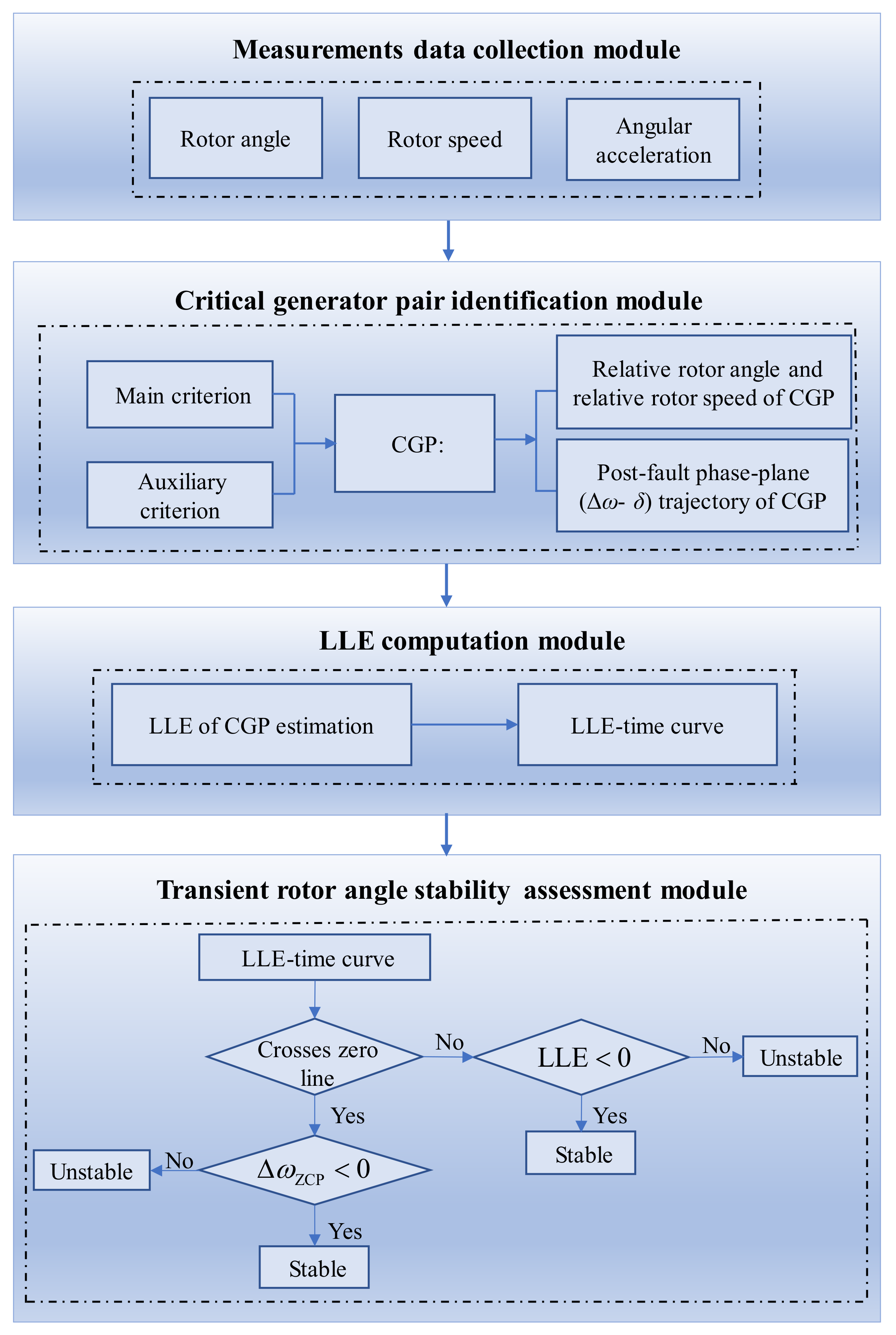
3.4. Online Rotor Angle Stability Assessment Scheme

The procedure of the proposed online rotor angle stability assessment is shown in Figure 4, which includes the measurement data collection module from WAMS, the CGP identification module, the LLE computation module, and the transient stability assessment module. Specifically,

(1)

When a fault is detected, the measurement data collection module is started to identify the CGPs. The relative rotor angle and rotor speed data of the CGPs are obtained in real time and the phase-plane trajectories of the CGPs are generated. It should be noted that the generator belonging to Ω_ncr is selected as the reference for the relative rotor angle and the rotor speed of the CGPs.

(2)

The LLE sequences for the relative rotor angle of the CGPs are calculated by the algorithm in Section 3.1.

(3)

The system rotor angle stability can be assessed by Criterion 1 and Criterion 2 proposed in Section 3.2. Note that the system is unstable if one of the CGPs is identified as unstable, and the system is stable if all of the CGPs are identified as stable.

4. Simulation Results

The proposed approach was tested on the IEEE-39 bus system and EGG. For the two power systems, the corresponding WAMS was assumed to have a hierarchical architecture [28]. The power systems were monitored with different areas, and the PMU measurements from different substations in different areas were collected, time aligned by the phasor data concentrator, and then submitted to the monitoring center. However, preserving full network observability may not be practically possible in large power systems [29]. Since the proposed approach performs online stability assessment only using the rotor angle and rotor speed data of generators, the rotor angle and rotor speed of the unobserved generators can be estimated by the dynamic state estimation algorithms, which can provide accurate and real-time estimation with respect to PMU measurements [30,31]. In our cases, the optimal PMU placement can be fulfilled based on the maximization of the determinant of the empirical observability, per Gramian in [32], where the obtained optimal PMU placements for generators can still guarantee good observability under a small or large disturbance. The sampling frequency of the PMU measurements used for the calculation of the LLE is 2 samples per cycle, i.e., 120 samples per second.

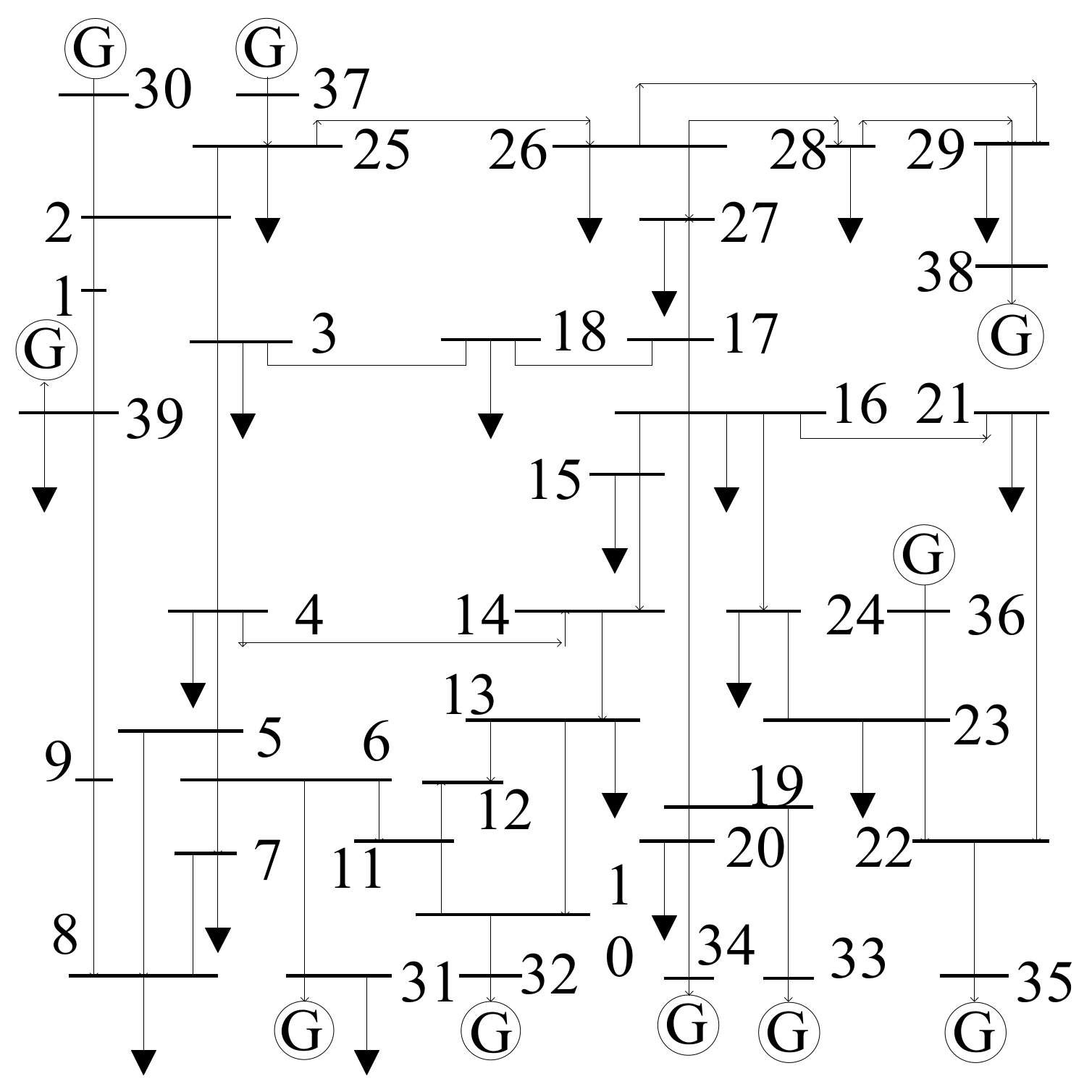
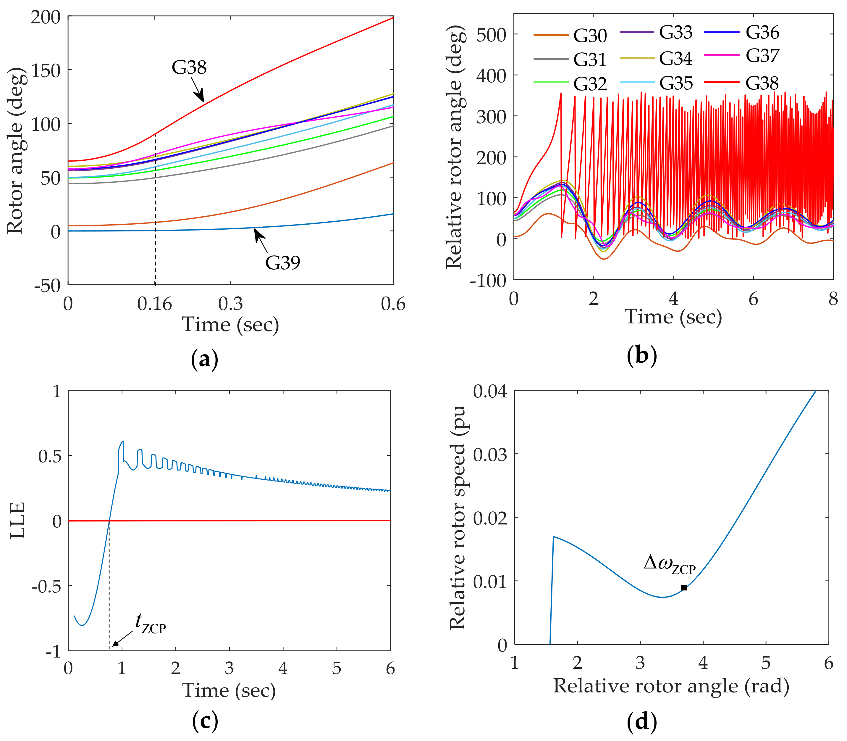
4.1. IEEE-39 Bus System

The diagram of the IEEE-39 bus test system is shown in Figure 5. Parameters about this system can be found in Reference [25]. The fourth-order transient model is used for generators. All loads are represented in a ZIP model, and the ratios of the constant current, constant resistance, and constant power loads are 0.5, 0.3, and 0.2, respectively. The three-phase to ground fault occurs on the line connecting buses 26 and 29 at time 0 s, and the fault is cleared at 7.5 cycles and 8 cycles for Case 1 and Case 2, respectively. By using the proposed CGP identification algorithm, the generator pair 38-39 is identified as the CGP for both cases.

Case 1: According to the time domain simulation (TDS), the system is critical stable when the fault clearing time is 7.5 cycles. Figure 6a,b are the TDS results. From the relative rotor angle curves in Figure 6b, it is found that the relative rotor angle of the CGP tends to be stable after a long period of oscillations. From the LLE evolution shown in Figure 6c, it can be easily seen that the LLE–time curve for the CGP crosses the zero line. The relative rotor speed at time t_ZCP for the CGP, shown as in Figure 6d, is less than zero, i.e., Δω_ZCP < 0. According to the proposed transient stability criterion, the system is stable, and the moment of the transient stability identified for the CGP is t_ZCP = 0.88 s. On the other hand, the earliest time of identifying the transient stability is more than 4 s by the traditional LLE-based method in [22], just according to the LLE evolution depicted in Figure 6c. Furthermore, from the F area marked in the phase-plane trajectory shown in Figure 6d, it can be found that the trajectory changes from concave to convex, resulting in an incorrect judgement that the system is unstable with the conventional method based on the phase-plane trajectory in [33], where the rotor angle stability are detected just according to the concavity and convexity of the phase-plane trajectory. From this perspective, our proposed stability assessment approach is more reliable, and will not be affected by the irregular changes of the phase-plane trajectory.

Case 2: According to the TDS, the system is critical unstable when the fault clearing time is 8 cycles. Figure 7a,b are the TDS results. From the relative rotor angle curves in Figure 7b, it is seen that the relative rotor angles of the CGP shows the first-swing instability after fault. From the LLE evolution shown in Figure 7c, it can be found that the LLE curve for the CGP crosses the zero line. The relative rotor speed at time t_ZCP for the CGP (shown in Figure 7d) is greater than zero, i.e., Δω_ZCP > 0. According to the proposed transient stability criterion, the system is unstable, and the moment of stability identified for the CGP is 0.87 s, i.e., the time needed to identify the transient rotor angle instability is only 0.71 s after clearing fault. In contrast, for the traditional LLE-based method in [22], a longer time is needed to observe the final sign of the LLE evolution depicted in Figure 7c, which identifies the rotor angle instability. Therefore, the system would be out-of-step before emergency control measures can be taken if the rotor angle stability is assessed by the proposed method in [22].

Furthermore, to verify the accuracy and effectiveness of the proposed assessment scheme for transient stability, the results assessed by the proposed approach, TDS, and the traditional LLE-based approach in [22] were compared. The comparisons of the simulation results for the fault scenario mentioned above with different fault clearing time are summarized in

Table 1. The comparisons of the simulation results obtained by different assessment approaches for the IEEE-39 bus system.

Tc 1 (cycles)	CGP	TDS	The Proposed Approach			Only by LLE–t Curve
			Stability Assessment Results	tac 2 (s)	ΔωZCP (rad)	Stability Assessment Results	LLE at t = 4 s
5.5	G38-G39	stable	stable	0.54	−0.0054	stable	−0.0560
6	G38-G39	stable	stable	0.56	−0.0056	stable	−0.0076
6.5	G38-G39	stable	stable	0.58	−0.0057	stable	−0.0631
7	G38-G39	stable	stable	0.62	−0.0061	unstable	0.0075
7.5	G38-G39	stable	stable	0.73	−0.0086	unstable	0.0141
8	G38-G39	unstable	unstable	0.71	0.0089	unstable	0.1069
8.5	G38-G39	unstable	unstable	0.55	0.0114	unstable	0.0947
9	G38-G39	unstable	unstable	0.44	0.0135	unstable	0.1064
9.5	G38-G39	unstable	unstable	0.36	0.0156	unstable	0.0937
10	G38-G39	unstable	unstable	0.29	0.0176	unstable	0.1054

¹ “T_c” denotes fault clearing time. ² “t_ac” denotes assessment time.

, which proves that the proposed scheme can assess the transient rotor angle stability accurately and rapidly. Moreover, the critical stable condition and the critical unstable condition can be distinguished accurately by the proposed approach. It should also be observed that the transient stability assessment time ranges from 0.29 s to 0.73 s, which indicates the rapidity of the proposed method. On the other hand, the assessment results obtained by the method in [22] for the cases of T_c = 7 cycles and T_c = 7.5 cycles are incorrect since it only ensures the signs of the LLEs at t = 4 s. Meanwhile, the stability assessment time needed for the unstable cases are much shorter than the time needed for the stable cases, so that the proposed approach is appropriate for being used in the real-time emergency control in order to avoid out-of-step splitting in power system. Furthermore, it can be seen that the longer fault clearing time leads to a less transient stability assessment time for unstable conditions. Figure 8 shows the LLE–time curves with different fault clearing times corresponding to Table 1. It can be seen that both of the stability assessment results obtained by the proposed approach and the LLE evolution method are accurate. However, most of the LLE–time curves fluctuate between positive and negative values for quite a long time. Therefore, it will take a long time to assess the rotor angle stability with the proposed approach in [22].

In the simulations of the IEEE-39 bus system, the identification of the CGP needs to be performed once and the auxiliary criterion does not need to be executed. The calculation time for the identification of the CGPs ranges from 0.015 ms to 0.035 ms, and the calculation time of the LLE for each sampling step ranges from 0.01 ms to 0.03 ms. Therefore, the largest total computing time for each sampling step is less than 10⁻⁴ s, which fully satisfies online computing demand.

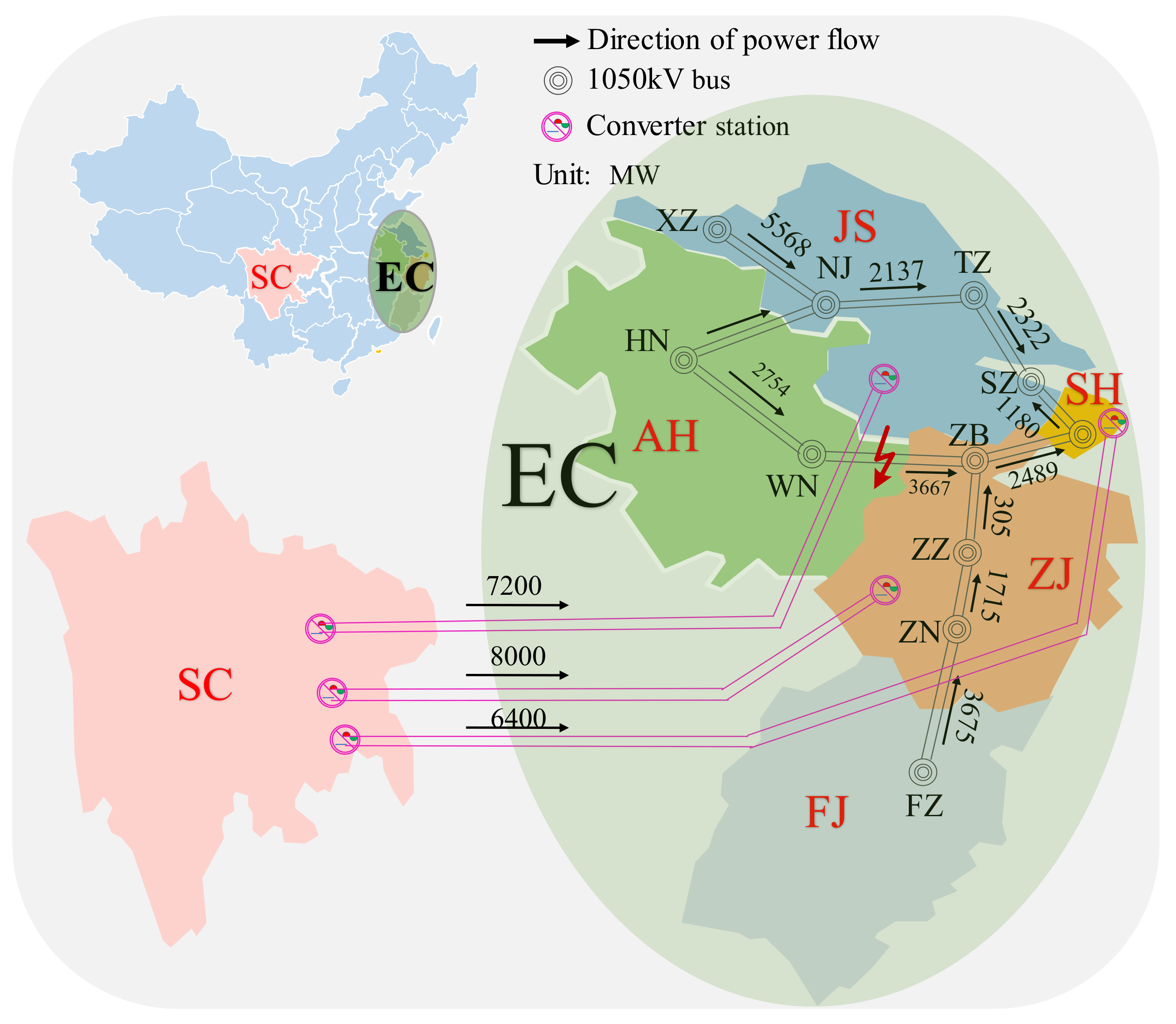
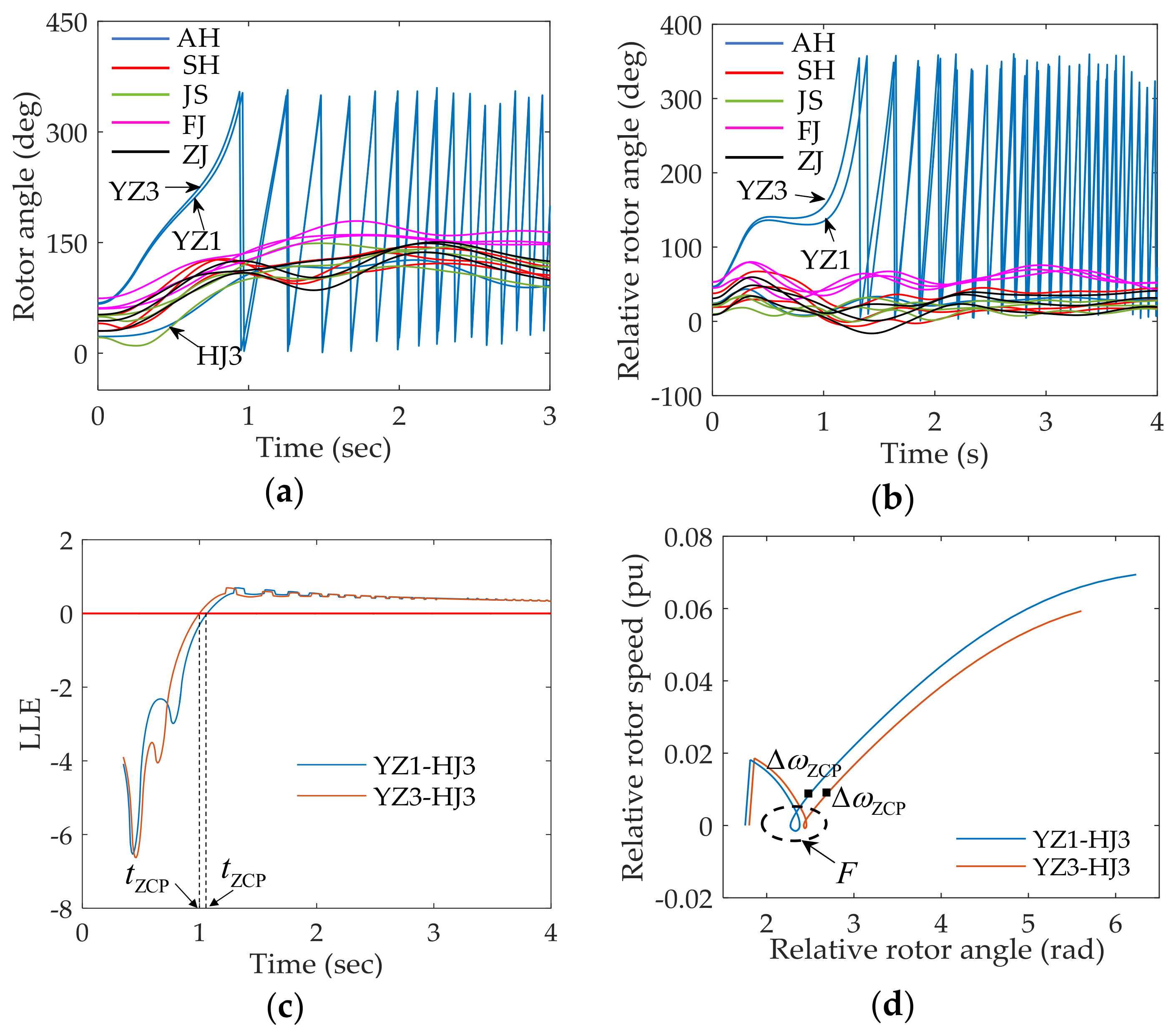
4.2. Real-World Power System

To evaluate the applicability of the proposed scheme, ECG—known as one of the ultrahigh voltage AC/DC hybrid power grids—was selected as a realistic test system. It is a large-scale multi-area interconnected power system composed of Anhui (AH), Jiangsu (JS), Shanghai (SH), Zhejiang (ZJ), and Fujian (FJ) provincial and municipal grids. The backbone network of ECG is shown in Figure 9. The number of the generators in ECG is 546, and the loads are described by different proportions of constant resistance load model and induction motors. The three-phase to ground fault occurs on the tie-line connected AH power grid and ZJ power grid, i.e., the transmission 1050 kV line interconnecting buses WN and ZE at time 0 s, and the fault is cleared after a duration of 12 cycles and 12.5 cycles for Case 3 and Case 4, respectively. By using the proposed CGP identification algorithm, the generator pairs YZ1-HJ3 and YZ3-HJ3 (YZ1 and YZ3 are the generators in the AH power grid, and HJ3 is the generator in the JS power grid are identified as the CGPs for both cases.

Case 3: According to the TDS, the system is critical stable when the fault clearing time is 12 cycles. Figure 10a,b are the TDS results. According to the relative rotor angle curves of the CGPs shown in Figure 10b, the CGPs finally tends to be stable. From the LLE evolution shown in Figure 10c, it can be easily seen that the LLE–time curves for both the CGPs cross the zero line. The relative rotor speed at time t_ZCP for both the CGPs, shown in Figure 10d, are less than zero, i.e., Δω_ZCP < 0. According to the proposed transient stability criterion, the system is stable, and the moments of the stability assessed for YZ1-HJ3 and YZ3-HJ3 are t_ZCP = 0.77 s and t_ZCP = 0.78 s, respectively, whereas the earliest identifying time is about 3 s by the method in [22], just according to the LLE evolution depicted in Figure 10c. Furthermore, from the phase-plane trajectory in F area shown in Figure 10d, it can be observed that the trajectory changes from concave to convex, resulting in an incorrect judgement that the system is unstable with the conventional phase-plane -based method in [33].

Case 4: According to the TDS, the system is critical unstable when the fault clearing time is 12.5 cycles. The fault duration of 12.5 cycles causes six unstable generators in AH power grid. Figure 11a,b are the TDS results. From the relative rotor curves shown in Figure 11b, both the CGPs show transient instability after fault. From the LLE evolution shown in Figure 11c, it can be easily seen that the LLE–time curves for both the CGPs cross the zero line. As can be seen in Figure 11d, Δω_ZCP > 0 for both the CGPs. According to the proposed transient stability criterion, the system is unstable, and the moments of stability identified for YZ1-HJ3 and YZ3-HJ3 are t_ZCP = 1.08 s and t_ZCP = 1.01 s, respectively. Therefore, the rotor angle stability assessment time for the system is 0.83 s after clearing fault. For comparison, the earliest identifying time is about 3 s by using the method in [22], just according to the LLE evolution depicted in Figure 11c. Moreover, the trajectory mutations occur in F area, as shown in Figure 11d. If the rotor angle stability is assessed by using the method in [34], where the first derivative of the phase-plane trajectory is used to identify the rotor angle stability, the identification results are easily affected by the trajectory mutations. Instead, the proposed approach can always provide a reliable assessment even when phase-plane trajectory mutations occur.

The transient stability assessment results of ECG by using the proposed approach, TDS, and the proposed method in [22] are compared. The comparisons for the above fault scenario with different fault clearing times are presented in

Table 2. The comparisons of the simulation results obtained by different assessment approaches for ECG.

Tc (cycles)	CGP	TDS	The Proposed Approach			Only by LLE–t Curve
			Stability Assessment Results	tac (s)	ΔωZCP (rad)	Stability Assessment Results	LLE at t = 5 s
10	YZ1-HJ3	stable	stable	0.28	−0.0094	stable	−0.2229
	YZ3-HJ3	stable	stable	0.29	−0.0101	stable	−0.2238
10.5	YZ1-HJ3	stable	stable	0.31	−0.0105	stable	−0.2228
	YZ3-HJ3	stable	stable	0.32	−0.0111	stable	−0.2235
11	YZ1-HJ3	stable	stable	0.37	−0.0111	stable	−0.2240
	YZ3-HJ3	stable	stable	0.38	−0.0115	stable	−0.2246
11.5	YZ1-HJ3	stable	stable	0.44	−0.0115	unstable	0.0028
	YZ3-HJ3	stable	stable	0.44	−0.0114	unstable	0.0033
12	YZ1-HJ3	stable	stable	0.53	−0.0111	unstable	0.0087
	YZ3-HJ3	stable	stable	0.54	−0.0112	unstable	0.0090
12.5	YZ1-HJ3	unstable	unstable	0.73	0.0087	unstable	0.1653
	YZ3-HJ3	unstable	unstable	0.71	0.0090	unstable	0.1642
13	YZ1-HJ3	unstable	unstable	0.50	0.0090	unstable	0.1673
	YZ3-HJ3	unstable	unstable	0.48	0.0092	unstable	0.1661
13.5	YZ1-HJ3	unstable	unstable	0.40	0.0091	unstable	0.1668
	YZ3-HJ3	unstable	unstable	0.39	0.0096	unstable	0.1656
14	YZ1-HJ3	unstable	unstable	0.34	0.0095	unstable	0.1641
	YZ3-HJ3	unstable	unstable	0.33	0.0098	unstable	0.1630
14.5	YZ1-HJ3	unstable	unstable	0.30	0.0104	unstable	0.1653
	YZ3-HJ3	unstable	unstable	0.28	0.0106	unstable	0.1642

. From Table 2, it is seen that the proposed stability assessment scheme can identify the real power system stability reliably and rapidly. It is demonstrated that the proposed scheme can provide an effective premise for emergency control to further avoiding blackout in real power systems. Moreover, both the critical stable condition and the critical unstable condition can be clearly identified by the proposed approach. Meanwhile, it can be observed that the stability identification time ranges from 0.28 s to 0.73 s, which indicates the rapidity of the proposed approach applied to the real power grid. In contrast, for the traditional LLE-based method in [22], the stability assessment results for the cases of T_c = 11.5 cycles and T_c = 11.5 cycles are incorrect if only according to the signs of the LLEs at t = 5 s, so that it needs take a relative longer time to observe the final sign of the LLE evolution to identify the rotor angle instability. Therefore, the system would be out-of-step before emergency control measures can be taken if the rotor angle stability is assessed by the proposed method in [22]. Figure 12 shows the LLE–time curves with different fault clearing time corresponding to Table 2. It can be seen that most of the LLE–time curves fluctuate between positive and negative values for quite a long time, and the observation time should be more than 6 s for the stable condition assessment by using the method in [22], just by monitoring the LLE evolutions.

In the simulations of ECG, the identification for each CGP needs to be performed once and the auxiliary criterion does not need to be executed. The calculation time for the identification of the CGPs ranges from 0.055 ms to 0.15 ms, and the calculation time of LLE for each sampling step ranges from 0.015 ms to 0.05 ms. Therefore, the largest total computing time for each sampling step is less than 0.2 ms, which indicates that the proposed assessment scheme can satisfy online computing demand for the large power system.

5. Discussions

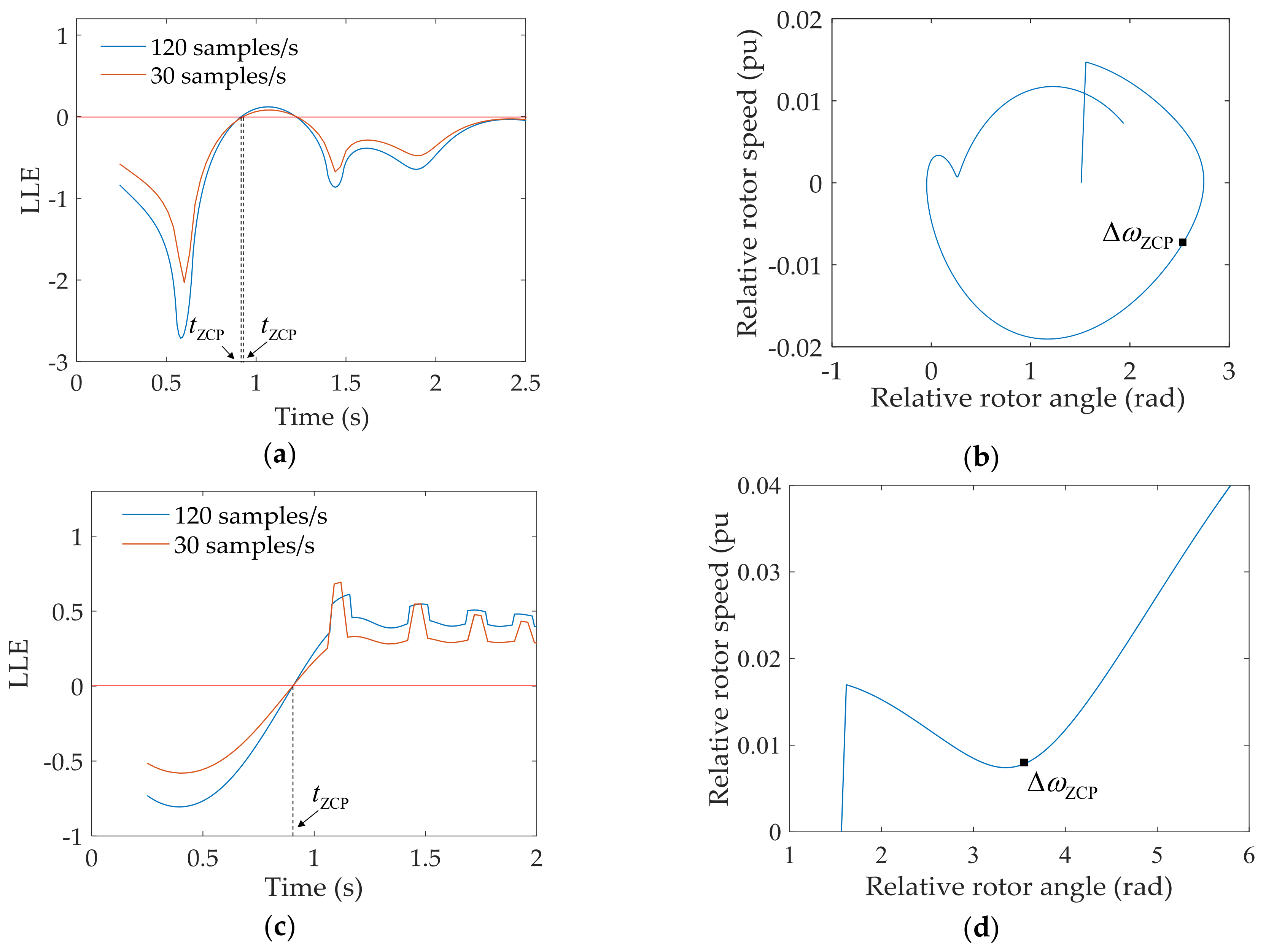
5.1. Effect of Sampling Rate

The sampling rate is an important aspect to be considered when implementing the online rotor angle stability assessment by using the PMU measurements. However, since the proposed approach only needs a small number of samples, the sampling rate has no significant effect on the assessment results. The realistic sampling rate for modern PMU ranges from 30 samples per second to 120 samples per second [32,35]. Figure 13 shows the rotor angle stability assessment results of different sampling rates for Case 1 and Case 2. From Figure 13, it can be clearly observed that the rapidity and correctness of the rotor angle assessment are not affected by the sampling rate with the proposed approach. Moreover, the dynamic state estimation can be realized in real time [30], which satisfies the requirement of the proposed approach.

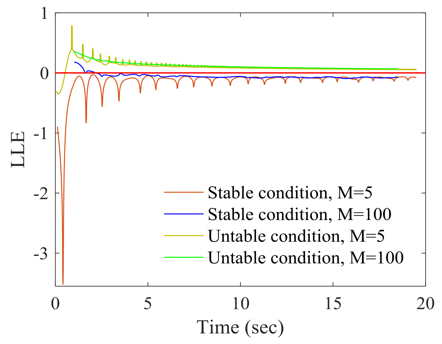
5.2. Effect of Initial Conditions

For the implementation of the proposed approach, the numbers of initial conditions (M) need to be determined. The appropriate size of the initial conditions is critical for accurate, reliable, and timely assessment. Figure 14 gives the assessment results of different M values for Case 1 and Case 2. (The colored squares in Figure 14b,d denote Δω_ZCP.) In the simulation, the sampling rate is 120 samples per second. From Figure 14, it can be observed that the larger M value leads to a faster assessment, and about 0.04 s decreases in stability assessment for every 5 increases in the value of M. Therefore, the rapidity of stability assessment can be improved by increasing M appropriately. However, M cannot be increased immoderately due to the proposed assessment approach being based on a small number for M. If M is too big, it may result in an inaccurate assessment for the proposed approach. According to extensive simulations and considering the speed of the data updating of PMUs, the appropriate size of M is 100–200 ms so that both the accuracy and rapidity of stability assessment can be ensured.

5.3. Discussions on the Differences from the Traditional LLE-Based Approach

The differences of the approach proposed in this paper from the approach in [22] can be summarized as:

(1)

Reference [22] requires the LLE–time curves of the relative rotor angles for all possible GPs. Instead, our proposed approach needs only the LLE–time curves of the CGPs.

(2)

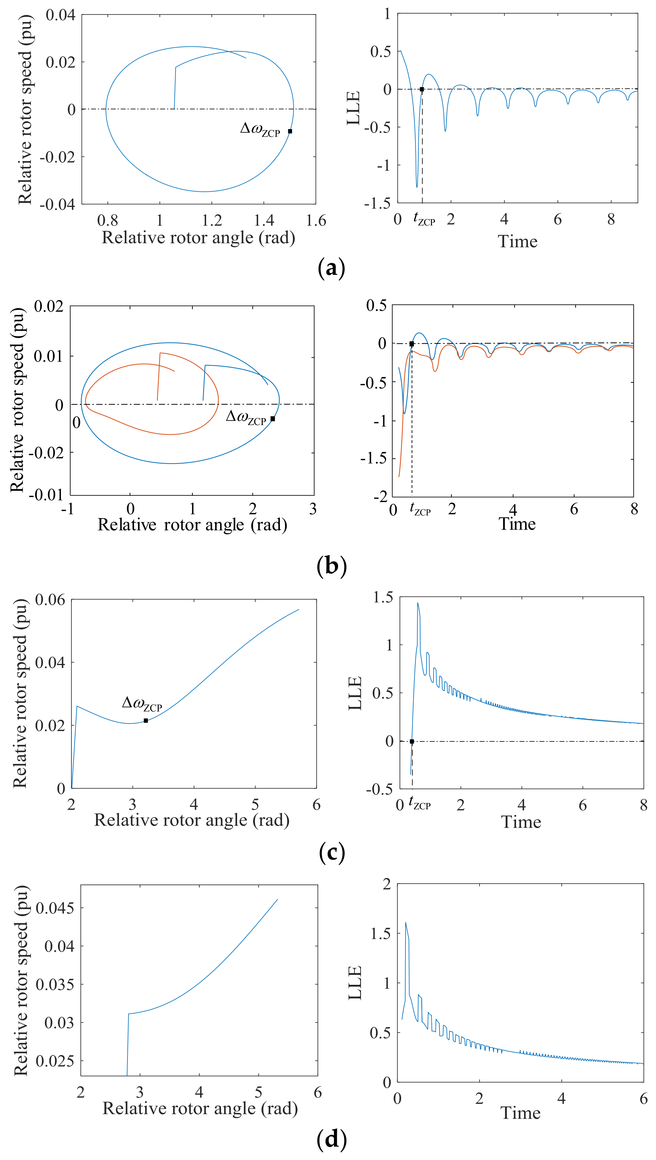
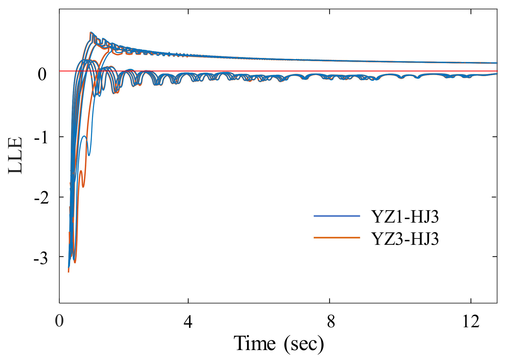
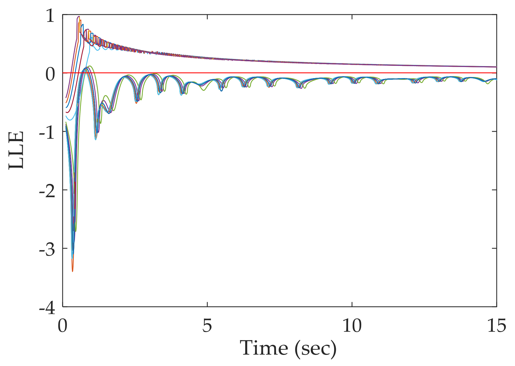
Reference [22] requires sufficient length of calculation time because the LLE estimated by the algorithm usually fluctuates between negative and positive values for quite a long time. In this paper, the calculation time length for each GGP is usually less than 1 s because the rotor angle stability can be assessed when the LLE–time curve crosses the zero line from negative to positive for the first time.

(3)

In this paper, the mathematical model between the LLE value and the rotor speed is established, and the proposed stability criterion combines the mathematical model with the dynamic characteristics of the phase-plane trajectory to guarantee the accuracy and the rapidity of the proposed stability criterion. However, Reference [22] only considers the signs of the LLE evolution as stability criterion. As a result, the stability assessment time is long, and the assessment results may be inaccurate because the calculation window and the sampling rates have a great effect on the LLE estimation.

6. Conclusions

In this paper, a model-free approach is proposed to assess transient rotor angle stability online based on the LLE and the rotor speed. By establishing the mathematical relationship between the LLE values and the rotor speed, we have presented a novel stability criterion that can be applied online to identify the rotor angle stability of a power system with WAMS measurements. The proposed approach does not need a long time calculation to observe the final signs of the LLE–time curves. Furthermore, an algorithm to identify the CGPs as the observation objective to assess the power system rotor angle stability is proposed. The proposed approach has successfully been performed on the IEEE-39 test system and ECG (546-bus system). Among all the simulation cases, the rotor angle stability can be assessed within 0.73 s, and the shortest time needed for the rotor angle stability assessment is only 0.28 s. Moreover, the total computing time for transient stability assessment is less than 10⁻³ s, which indicates that the proposed approach is fast enough to satisfy the online calculating requirement for large power system.

Future investigations are underway to incorporate the proposed approach and emergency control to prevent power systems from entering an unstable state.

References

1. Kundur, P.; Paserba, J.; Ajjarapu, V.; Andersson, G.; Bose, A.; Canizares, C.; Hatziargyriou, N.; Hill, D.; Stankovic, A.; Van Cutsem, T.; et al. Definition and classification of power system stability IEEE/CIGRE joint task force on stability terms and definitions. IEEE Trans. Power Syst. 2004, 19, 1387–1401. [Google Scholar]
2. Su, H.Y.; Liu, T.Y. GECM-based voltage stability assessment using wide-area synchrophasors. Energies 2017, 10, 1601. [Google Scholar] [CrossRef]
3. Zhao, J.; Zhang, G.; Das, K.; Korres, G.N.; Manousakis, N.M.; Sinha, A.K.; He, Z. Power system real-time monitoring by using PMU-based robust state estimation method. IEEE Trans. Smart Grid 2016, 7, 300–309. [Google Scholar] [CrossRef]
4. Vu, T.L.; Turitsyn, K. Lyapunov functions family approach to transient stability assessment. IEEE Trans. Power Syst. 2016, 31, 1269–1277. [Google Scholar] [CrossRef]
5. Reddy, S.S.; Prathipati, K.; Lho, Y.H. Transient stability improvement of a system connected with wind energy generators. Int. J. Emerg. Electr. Power Syst. 2017, 18, 1–15. [Google Scholar] [CrossRef]
6. Zadkhast, S.; Jatskevich, J.; Vaahedi, E. A multi-decomposition approach for accelerated time-domain simulation of transient stability problems. IEEE Trans. Power Syst. 2015, 30, 2301–2311. [Google Scholar] [CrossRef]
7. Fang, D.Z.; Chung, T.S.; Zhang, Y.; Song, W. Transient stability limit conditions analysis using a corrected transient energy function approach. IEEE Trans. Power Syst. 2000, 15, 804–810. [Google Scholar] [CrossRef]
8. Wang, B.; Fang, B.; Wang, Y.; Liu, H.; Liu, Y. Power system transient stability assessment based on big data and the core vector machine. IEEE Trans. Smart Grid 2016, 7, 2561–2570. [Google Scholar] [CrossRef]
9. Reddy, S.S.; Rathnam, C.S. Optimal power flow using glowworm swarm optimization. Int. J. Electr. Power Energy Syst. 2016, 80, 128–139. [Google Scholar] [CrossRef]
10. Gurusinghe, D.R.; Rajapakse, A.D. Post-disturbance transient stability status prediction using synchrophasor measurements. IEEE Trans. Power Syst. 2016, 31, 3656–3664. [Google Scholar] [CrossRef]
11. Bhui, P.; Senroy, N. Real-time prediction and control of transient stability using transient energy function. IEEE Trans. Power Syst. 2017, 32, 923–934. [Google Scholar] [CrossRef]
12. Oluic, M.; Ghandhari, M.; Berggren, B. Methodology for rotor angle transient stability assessment in parameter space. IEEE Trans. Power Syst. 2017, 32, 1202–1211. [Google Scholar]
13. Amraee, T.; Ranjbar, S. Transient instability prediction using decision tree technique. IEEE Trans. Power Syst. 2013, 28, 3028–3037. [Google Scholar] [CrossRef]
14. AL-Masri, A.N.; Ab Kadir, M.Z.A.; Hizam, H.; Mariun, N. A novel implementation for generator rotor angle stability prediction using an adaptive artificial neural network application for dynamic security assessment. IEEE Trans. Power Syst. 2013, 28, 2516–2525. [Google Scholar] [CrossRef]
15. Zhou, Y.; Wu, J.; Ji, L.; Hao, L. A hierarchical method for transient stability prediction of power systems using the confidence of a SVM-based ensemble classifier. Energies 2016, 9, 778. [Google Scholar] [CrossRef]
16. Li, Y.; Yang, Z. Application of EOS-ELM with binary Jaya-based feature selection to real-time transient stability assessment using PMU Data. IEEE Access 2017, 25, 23092–23101. [Google Scholar] [CrossRef]
17. James, J.Q.; Hill, D.J.; Lam, A.Y.; Gu, J.; Li, V.O. Intelligent time-adaptive transient stability assessment system. IEEE Trans. Power Syst. 2018, 33, 1049–1058. [Google Scholar]
18. Liu, C.W.; Thorp, J.S.; Lu, J.; Thomas, R.J.; Chiang, H.D. Detection of transiently chaotic swings in power systems using real-time phasor measurements. IEEE Trans. Power Syst. 1994, 9, 1285–1292. [Google Scholar]
19. Khaitan, S.K.; McCalley, J.D. VANTAGE: A Lyapunov exponents based technique for identification of coherent groups of generators in power systems. Electr. Power Syst. Res. 2013, 105, 33–38. [Google Scholar] [CrossRef]
20. Yan, J.; Liu, C.C.; Vaidya, U. PMU-based monitoring of rotor angle dynamics. IEEE Trans. Power Syst. 2011, 26, 2125–2133. [Google Scholar] [CrossRef]
21. Wadduwage, D.P.; Wu, C.Q.; Annakkage, U.D. Power system transient stability analysis via the concept of Lyapunov Exponents. Electr. Power Syst. Res. 2013, 104, 183–192. [Google Scholar] [CrossRef]
22. Dasgupta, S.; Paramasivam, M.; Vaidya, U.; Ajjarapu, V. PMU-based model-free approach for real-time rotor angle monitoring. IEEE Trans. Power Syst. 2015, 30, 2818–2819. [Google Scholar] [CrossRef]
23. Dasgupta, S.; Paramasivam, M.; Vaidya, U.; Ajjarapu, V. Real-time monitoring of short-term voltage stability using PMU data. IEEE Trans. Power Syst. 2013, 28, 3702–3711. [Google Scholar] [CrossRef]
24. Skokos, C.H.; Gottwald, G.A.; Laskar, J. Chaos Detection and Predictability; Springer: Berlin/Heidelberg, Germany, 2016; pp. 123–135. [Google Scholar]
25. Pai, M.A. Energy Function Analysis for Power System Stability; Kluwer Academic Publishers: Boston, MA, USA, 1989. [Google Scholar]
26. Wang, L.; Girgis, A.A. A new method for power system transient instability detection. IEEE Trans. Power Deliv. 1997, 12, 1082–1089. [Google Scholar] [CrossRef]
27. Haque, M.H.; Rahim, A.H.M.A. Determination of first swing stability limit of multimachine power systems through taylor series expansions. IEE Proc. C 1989, 136, 373–380. [Google Scholar] [CrossRef]
28. He, M.; Vittal, V.; Zhang, J. Online dynamic security assessment with missing PMU measurements: A data mining approach. IEEE Trans. Power Syst. 2013, 28, 1969–1977. [Google Scholar] [CrossRef]
29. Sun, K.; Qi, J.; Kang, W. Power system observability and dynamic state estimation for stability monitoring using synchrophasor measurements. Control Eng. Pract. 2016, 53, 160–172. [Google Scholar] [CrossRef]
30. Zhou, N.; Meng, D.; Huang, Z.; Welch, G. Dynamic state estimation of a synchronous machine using PMU data: A. comparative study. IEEE Trans. Smart Grid. 2015, 6, 450–460. [Google Scholar] [CrossRef]
31. Ariff, M.A.; Pal, B.C.; Singh, A.K. Estimating dynamic model parameters for adaptive protection and control in power system. IEEE Trans. Power Syst. 2015, 30, 829–839. [Google Scholar] [CrossRef]
32. Qi, J.; Sun, K.; Kang, W. Optimal PMU placement for power system dynamic state estimation by using empirical observability gramian. IEEE Trans. Power Syst. 2015, 30, 2041–2054. [Google Scholar] [CrossRef]
33. Wang, H.; Zhang, B.; Hao, Z. Response based emergency control system for power system transient stability. Energies 2015, 8, 13508–13520. [Google Scholar] [CrossRef]
34. Gu, Z.Y.; Yong, T.; Sun, H. An identification method for power system transient angle stability based on the trend of rotor speed difference-rotor angle difference. Proc. CSEE 2013, 33, 65–72. [Google Scholar]
35. Jones, K.D.; Pal, A.; Thorp, J.S. Methodology for performing synchrophasor data conditioning and validation. IEEE Trans. Power Syst. 2015, 30, 1121–1130. [Google Scholar] [CrossRef]
Figure 1. Typical features of the phase-plane trajectories of a generator pair (GP) after clearing fault with different fault-clearing times.
Energies 11 00958 g001
Figure 2. Largest Lyapunov exponent (LLE) calculated by using the model-free algorithm for different stability conditions with different M values.
Energies 11 00958 g002
Figure 3. Phase-plane trajectories after clearing fault and corresponding LLE–time curves of a GP under different stability conditions: (a) Stability Condition 1 and the corresponding LLE–time curve; (b) Stability Condition 2 and the corresponding LLE–time curve; (c) Stability Condition 3 and the corresponding LLE–time curve; (d) Stability Condition 4 and the corresponding LLE–time curve.
Energies 11 00958 g003
Figure 4. Flowchart of the proposed scheme for online transient rotor angle stability assessment.
Energies 11 00958 g004
Figure 5. Diagram of the IEEE-39 bus test system.
Energies 11 00958 g005
Figure 6. Simulation results for Case 1: (a) Rotor angle curves of generators after fault; (b) relative rotor angle curves after fault (G39 is the reference generator); (c) LLE–time curves; (d) phase-plane trajectories after clearing the fault.
Energies 11 00958 g006
Figure 7. Simulation results for Case 2: (a) Rotor angle curves of generators after fault; (b) relative rotor angle curves after fault (G39 is the reference generator); (c) LLE–time curves; (d) phase-plane trajectories after clearing the fault.
Energies 11 00958 g007
Figure 8. LLE–time curves with different fault clearing times for the mentioned fault scenario of the IEEE-39 bus test system.
Energies 11 00958 g008
Figure 9. Power flow diagram of East China Power Grid (ECG).
Energies 11 00958 g009
Figure 10. Simulation results for Case 3: (a) Rotor angle curves of generators after fault; (b) relative rotor angle curves after fault (HJ3 is the reference generator); (c) LLE–time curves; (d) phase-plane trajectories after clearing the fault.
Energies 11 00958 g010
Figure 11. Simulation results for Case 4: (a) Rotor angle curves of generators after fault; (b) relative rotor angle curves after fault (HJ3 is the reference generator); (c) LLE–time curves; (d) phase-plane trajectories after clearing the fault.
Energies 11 00958 g011
Figure 12. LLE–time curves with different fault clearing time for the mentioned fault scenario of ECG.
Energies 11 00958 g012
Figure 13. Simulation results of different sampling rates for Case 1 and Case 2. (a) LLE–time curves for Case 1; (b) phase-plane trajectory after clearing the fault of Case 1; (c) LLE–time curves for Case 2; (d) phase-plane trajectory after clearing the fault of Case 2.
Energies 11 00958 g013
Figure 14. Simulation results of different initial conditions for Case 1 and Case 2. (a) LLE–time curves for case 1; (b) phase-plane trajectory after clearing the fault of Case 1; (c) LLE–time curves for Case 2; (d) phase-plane trajectory after clearing the fault of Case 2.
Energies 11 00958 g014aEnergies 11 00958 g014b