Smart Hybrid Micro-Grid Integration for Optimal Power Sharing-Based Water Cycle Optimization Technique

Abstract

Micro-Grid (MG) with hybrid power resources can supply electric loads independently. In case of surplus power, the neighborhood micro-grids can be integrated together in order to supply the overloaded micro-grid. The challenge is to select the most suitable, optimal and preferable micro-grid within a distributed network, which consists of islanded MGs, to form that integration. This paper presents an intelligent decision-making criteria based on the Weighted Arithmetic Mean (WAM) of different technical indices, for optimal selection of micro-grids integration in case of overloaded event due to either unusual increase in consumed power or any deficiency in power generation. In addition, overloading is expected due to excess increase or decrease in weather temperature. This may lead to extreme increase of load due to increase of air conditioning or heating loads respectively. The proposed arithmetic mean determination based on six multi-objective indices, which are voltage deviation, frequency deviation, reliability, power loss in transmission lines, electricity price and CO₂ emission is applied. This work is developed through three main scenarios. The first scenario studies the effect of each index on the integrated micro-grid formation. The second scenario is the biased optimization analysis. In this stage, the optimal micro-grids integration is based on intentionally chosen multi-objective index weights to fulfil certain requirements. The third scenario targets the optimal selection of the multi-objective indices’ effectiveness weights for power system optimum redistribution. The sharing weights of each index will be optimally selected by Water Cycle Optimization Technique (WCOT) and Genetic Algorithm (GA) addressing the system optimal power sharing through optimum micro-grids re-formation (integration). WCOT and GA are simulated using MATLAB (R2017a, The MathWorks Ltd, Natick, MA, USA). The developed work is applied to a distributed network which consists of a five micro-grid tested system, with one overloaded micro-grid. The three modules are utilized for multi-objective analysis of different alternative micro-grids. Both WCOT and GA results are compared. In addition, it is investigated to find and validate the optimum solution. Final decision-making for optimal combination is determined, aiming to reach a perfect technical, economic and environmental solution. The results indicate that the optimal decision may be modified after each individual index weight exceeds a specific limit.

1. Introduction

Micro-grids (MGs) play a very important role in the technical, economical and environmental aspects of power system studies. Micro-grid is a distributed system network that merges (is constructed of) a power generation implemented by Distributed Generators (DGs), distributed energy resources (DERs), storage systems and loads. The DGs and DERs can be a combination of clean renewable energy and conventional fossil fuel resources [1]. MGs have a low development and implementation cost which involves power generation, storage and consumption, which can be developed, adapted, innovated and proposed through local technologies [2]. Smart grids are constructions of micro-grids which can operate in isolated or grid-connected modes [1]. The operation of MG modes is mainly controlled through a central controller, which has a power module protection and management coordination [2]. Although, at normal operation, each micro-grid supplies its own loads by its own distributed generators (which is called isolated mode), still there is connection to the grid by an Interconnecting Static Switch (ISS) which is normally open. Unfortunately, the topological structure of the distributed network can be changed due to natural disasters such as floods, hurricanes, blizzards or any extreme weather condition which may cause defects or increase the outages. Hurricane Sandy was one of those disasters that caused an outage for 15 states in the USA. The annual inflation adjusted cost is estimated at $25–$70 billion in the US [3].

In the case of overloading due to vulnerable and unexpected conditions in MG, power restoration of the distributed network is targeted. It can be processed through two methodologies. The first methodology depends on supporting the overloaded MG by utilizing under-frequency/voltage load shedding, energy storage system [4], or Distributed System Restoration (DSR). DSR restores the loads after any fault or blackout, by various solutions such as fuzzy logic [5,6], multi-agent systems [7], heuristic search [8], mathematical programming [9], expert systems [10], spanning tree search [11], distributed generators insertion by branch bound algorithm [12] and Mixed-Integer Linear Program (MILP) [13]. The second methodology relies on either interconnecting the overloaded MG to utility [14] or coupling it with the neighboring MGs [15], which can be done through ISS. ISS operates either on a centralized or decentralized mode based on the availability of the data communications [15]. The supervisory control approach to ensure the optimum coupling by ISS can be done by many methodologies like Droop Control Regulation (DCR) [16], stability improvement in the presence of constant power loads by a Lyapunov redesign controller [17], Load-to-Capacity (L2C) ratio [18], analysis of Small Signal Stability (SSS) [19], and cloud theory-based probabilistic method [20]. DCR is used to regulate the voltage and frequency to improve load sharing by droop coefficients [16]. L2C ratio depends on the communications among all MGs which is represented in two Auxiliary Controllable Loads (ACL) at the two sides of the ISS to alleviate transient current in the tie line between MGs [18]. The Analysis of Small Signal Stability (SSS) based on decision-making algorithm couples only two neighboring islanded MGs; and if the system is unstable the droop control coefficient can be changed to establish the coupling process as in [19]. The cloud theory-based probabilistic method based on decision-making algorithm depends on some indices and focuses on random different weights for each criteria [20].

The economic aspects perform an important role in electrical power system operation, management and control. Various studies consider the techno-economic assessment issues in improving the power system performance. Techno-economic assessment criteria tend to combine technical and economic solutions in order to optimize the operation of micro-grid by improving the reliability level based on sequential Monte Carlo simulations and maximizing the benefits associated with reliability services [21] or self-healing by different energy configuration of the network [22,23,24].

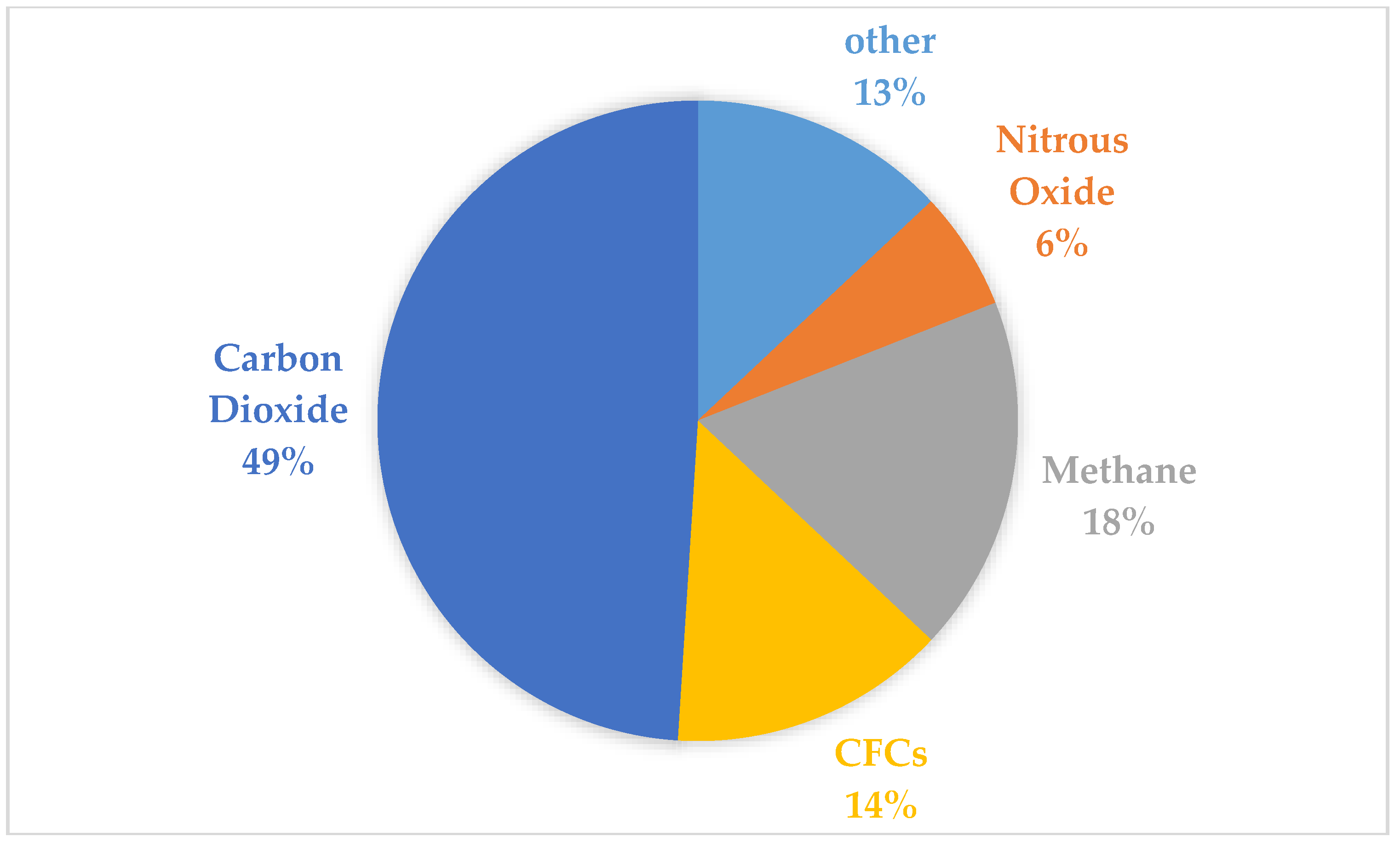
Carbon Dioxide emission (CO₂ emission in $/ton of CO₂) is one of the main critical global issues. The CO₂ emission resulting from fossil fuel burning is responsible for approximately 50% of the global warming. Its contribution to the greenhouse effect is clarified in Figure 1, where 1990 is the base year statistics, and the predictions cover a ten-year interval from 2000 to 2010 [25].

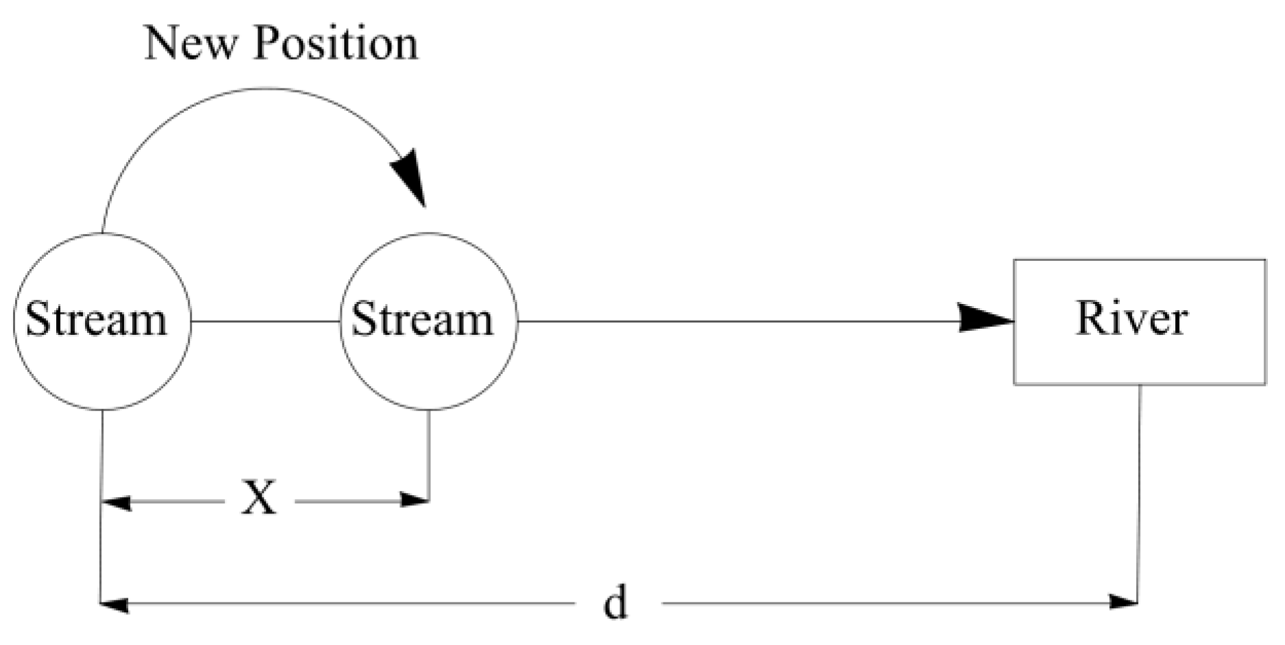
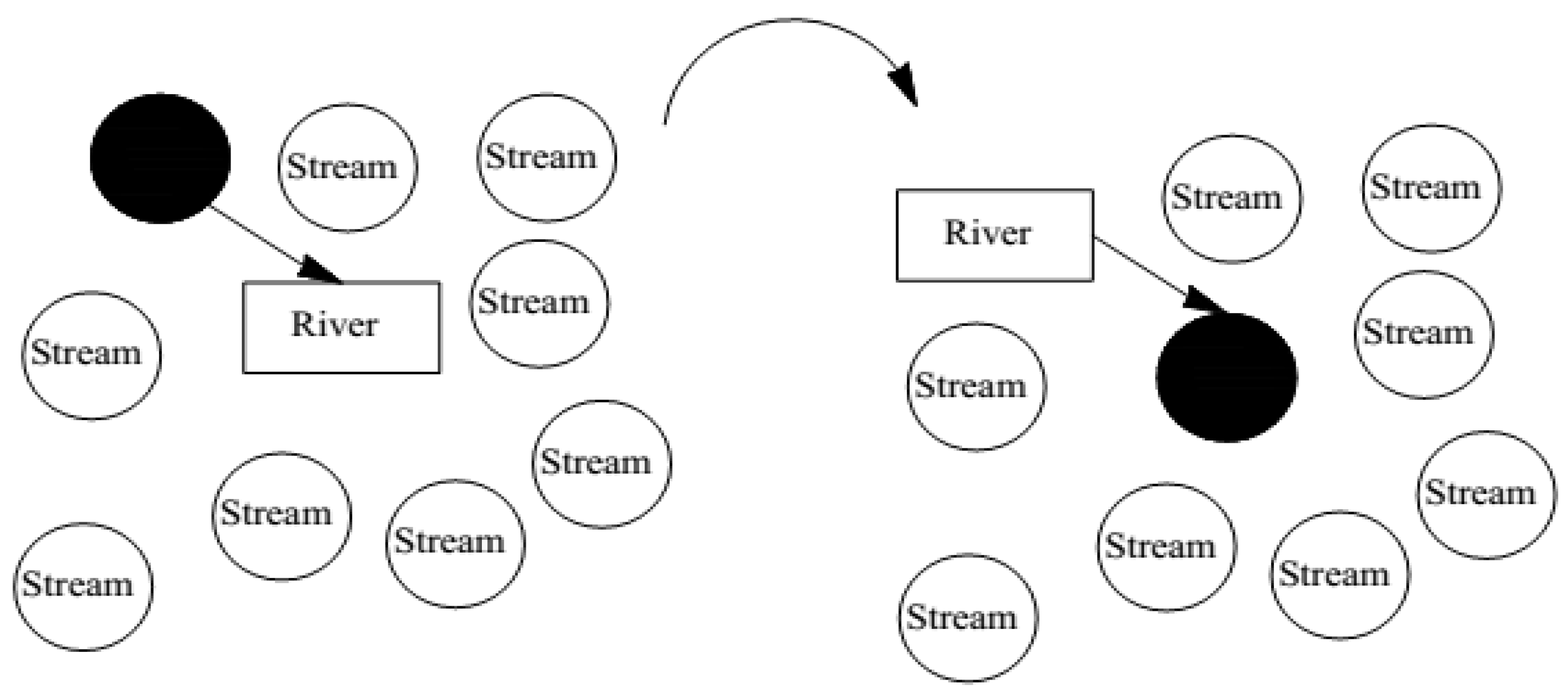
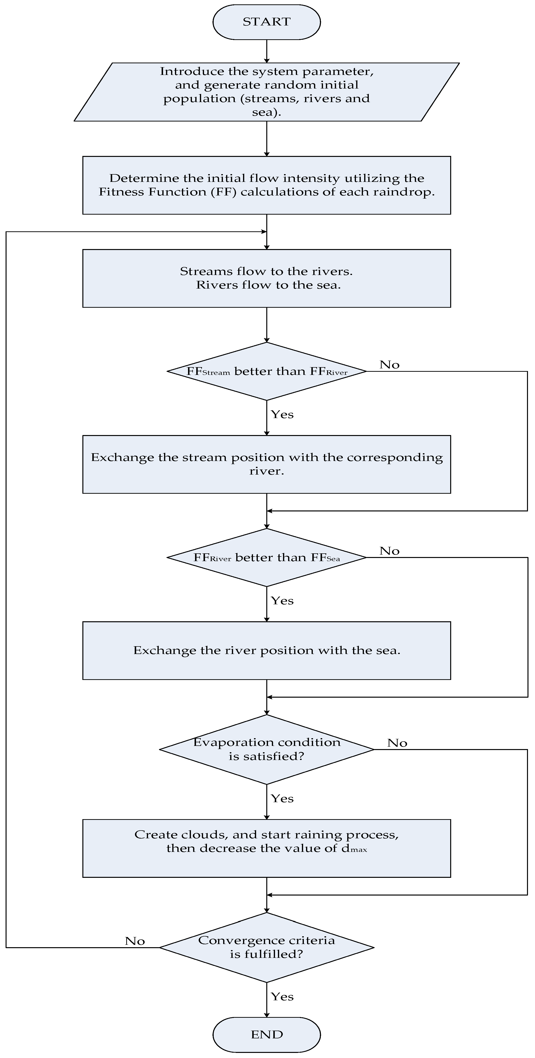
In this paper, the technical, environmental and economic optimum power sharing alternative which can supply the overloaded MG is studied based on the multi-objective indices for the decision-making criteria. The decision-making is based on sharing weights of the indices individually. The decision-making criteria are developed through two main strategies based on three scenarios. The basic analysis method is utilized in the first strategy, which consists of both the Equally Weighted Indices Scenario (EWIS) and the Intended Targeted Weighted Indices Scenario (ITWIS). The second strategy is based on the Intelligent Optimization Scenario (IOS) which utilizes the Water Cycle Optimization Technique (WCOT) [26] compared to Genetic Algorithm (GA). The Water Cycle Algorithm (WCA) efficiency has been proved in solving complex issues with the optimum solution compared to other optimization techniques like linear programing (LP), nonlinear programming (NLP) and practical swarm optimization (PSO) [27]

The paper is divided into five main sections. Section 2 illustrates the operation conditional flags and multi-objective indices for decision-making criteria. Section 3 provides an overview of the intelligent optimization scenarios (IOS). Section 4 illustrates Hybrid MG Integration Simulation and Results. Section 5 represents the paper conclusion.

2. Operation Conditional Flags and Multi-Objective Indices for Decision-Making Criteria

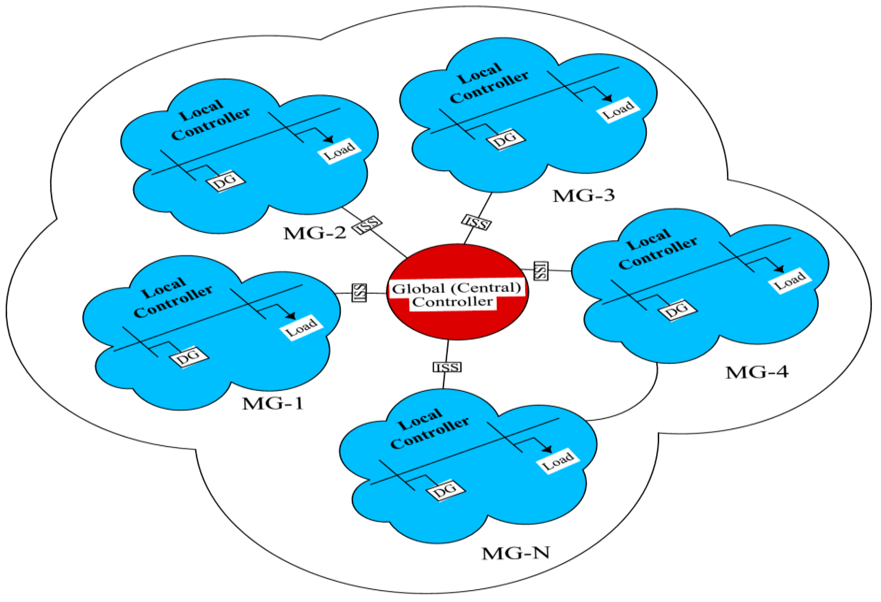
The distributed network shown in Figure 2 is constructed of N islanded micro-grids. Normally, each of them works in a stable way at steady state conditions. Each MG has a hybrid combination of Distributed Generation (DG) that consists of renewable energy resources in addition to the conventional fossil fuel resources. Under sudden abnormal conditions which lead to either power generation deficiency or overloading situation, an optimal decision should be made to select the most efficient, economical and environmental friendly MG integration alternative. The suggested optimal coupled alternative to the ill-MG may consist of only one MG or a set of integrated MGs.

For example, a distributed network, which is built of 3 MGs (N = 3), with overloaded MG (MG-1), has three power covering alternatives. The different alternatives are [{MG-2}, {MG-3} and {MG-2 & MG-3}]. Generally, if N_O is the overloaded MG in a distributed network, which has N MGs, then the available alternatives N_a are as follows

$$N_a=2^{N-N_0}-1$$

(1)

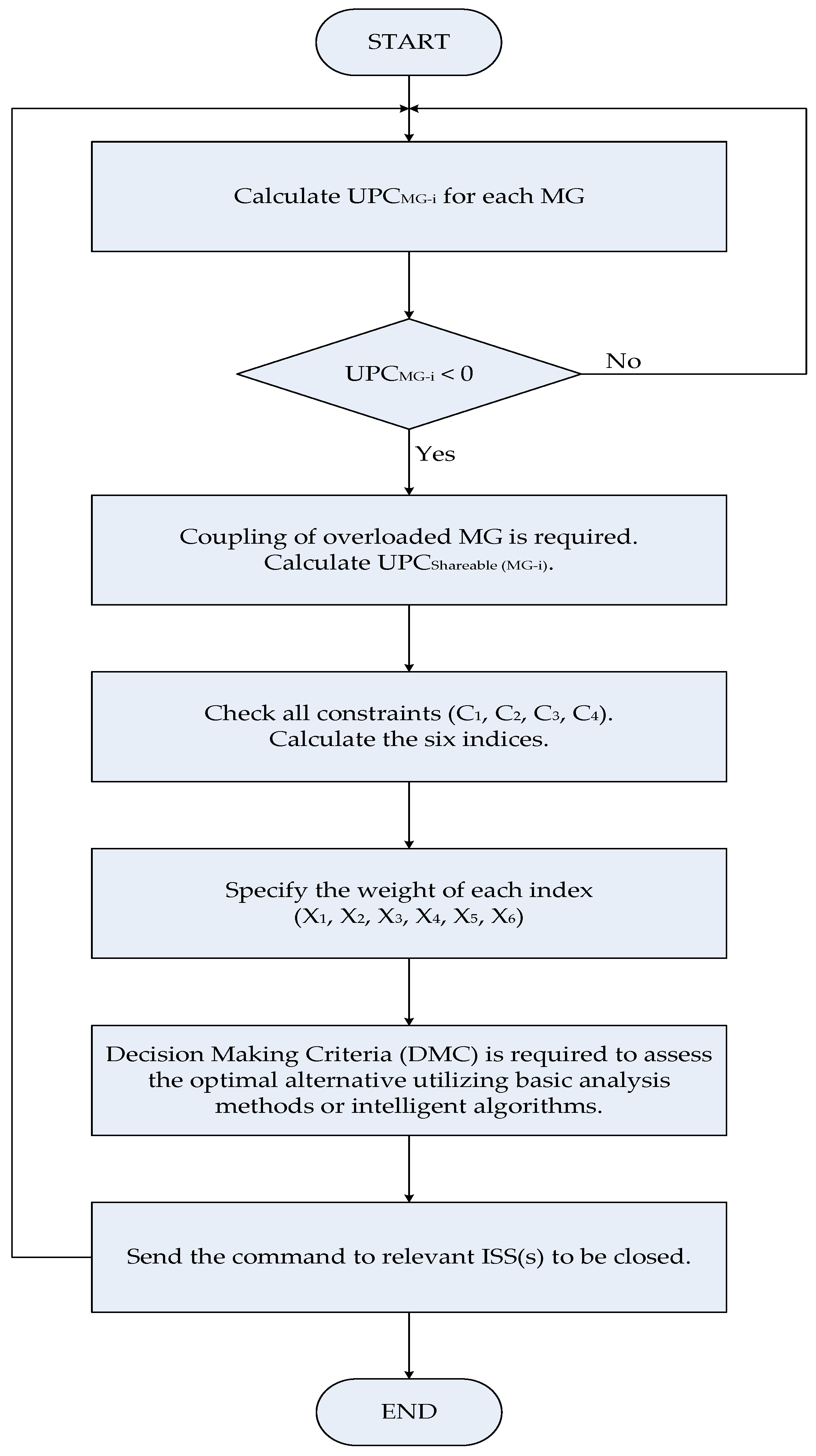
The global central controller is responsible for the optimal decision-making, based on the active generated and consumed power data collected from the local MG controllers. The decision signals are sent to the individual Interconnecting Static Switch (ISS) to be opened or closed according to the power re-distribution indices, after considering the operation conditional flags.

Four operation conditions should be checked for each MG to ensure its validity in supplying the ill-MG either alone or through a combined MG group.

2.1. Operation Conditional Flags

2.1.1. The Shareable Unused Power Capacity (UPC_Shareable) Flag (C₁)

The Unused Power Capacity (UPC) is calculated for each MG as

$$UP{C}_{MG-i}=P_{DG\left(MG-i\right)}-P_{LOAD\left(MG-i\right)}$$

(2)

where P_{DG (MG-i)} and P_{load (MG-i)} are the active generated power and the consumed power of micro-grid i respectively.

If UPC is less than zero, then this MG is overloaded. The Shareable Unused Power Capacity (UPC_Shareable) is calculated for all the remaining MG(s) as

$$UP{C}_{Shareable\left(MG-i\right)}=UP{C}_{\left(MG-i\right)}-\alpha P_{load\left(MG-i\right)}$$

(3)

where α is a safety margin for any sudden fault or disaster which may take place during the formation of the distributed network. It is suggested that α = 0.25 to save a generation margin equivalent to 25% of the MG’s consumed power in case of any emergency power extension.

As UPC_Shareable represents the UPC after assigning a safety margin, it is reserved to cover any sudden disturbance or overloading condition in the network. The condition for coupling the studied alternative with the ill-MG is that its UPC_Shareable must overcome the Power Deficiency Load (PDL), otherwise, the studied alternative may be combined with other MG sets. C₁ should be checked for each MG as follows:

$$C_1=\{\begin{array}{llllllll}0& & & & & & & if{\displaystyle \sum _{i=1}^{N_a}}UP{C}_{Shareable\left(MG-i\right)}<PD{L}_{MG-j}\\ 1& & & & & & & if{\displaystyle \sum _{i=1}^{N_a}}UP{C}_{Shareable\left(MG-i\right)}\ge PD{L}_{MG-j}\end{array}$$

(4)

where N_a is the number of MG(s) in the same alternative.

2.1.2. Interconnecting Static Switch (ISS) Flag (C₂)

The second condition flag is the availability of each MG. It illustrates the status of the ISS that indicates the tie to the overloaded MG.

$$C_2=\{\begin{array}{cccccccccc}0\hfill & & & & & & & ifMG\hfill & & \hfill vetoescoupling\\ 1\hfill & & & & & & & ifMG\hfill & & \hfill consentscoupling\end{array}$$

(5)

If C_2i flag is zero, MG-i cannot supply the overloaded MG or be shared with any other MG(s).

2.1.3. Voltage Deviation Flag (C₃)

Voltage deviation ($\Delta V$) is one of the main important conditions, which must be checked before MGs coupling, to be assured within a specific limit. It is defined by the maximum voltage difference between corresponding bus and nominal voltage (V_nominal) for each MG. This deviation should be kept within the limit of $\pm \Delta V_L=$ ±5% to avoid any failure or damage in the distributed system [28]:

$$\Delta V=Max\left(V_b-V_{nominal}\right)$$

(6)

where V_b is the voltage of bus-b in MG-i (in p.u.), with b $\in$ {1, 2, 3, …, N_bus}. V_nominal = 1 p.u.

$$C_3=\{\begin{array}{llllllll}0& & & & & & & if\Delta V_L<\Delta V<-\Delta V_L\\ 1& & & & & & & if\Delta V_L>\Delta V>-\Delta V_L\end{array}$$

(7)

2.1.4. Frequency Deviation Flag (C₄)

Frequency deviation ($\Delta F$) is the maximum frequency difference between the bus and the nominal frequency (F_nominal) of each MG. Deviation in frequency may lead to a disaster, so the maximum acceptable fluctuation is $\pm \Delta F_L$ = ±1% [29]. It is represented as

$$\Delta F=Max\left(F_b-F_{nominal}\right)$$

(8)

where F_b is the p.u. frequency bus-b in MG-i. F_nominal = 1 p.u.

The fourth studied condition is the frequency deviation, which must be studied to be confirmed within a certain range.

$$C_4=\{\begin{array}{llllllll}0& & & & & & & if\Delta F_L<\Delta F<-\Delta F_L\\ 1& & & & & & & if\Delta F_L>\Delta F>-\Delta F_L\end{array}$$

(9)

After inspecting the condition flags, the six evaluating indices should be studied to be the main assessment of the decision-making criteria.

2.2. Multi-Objective Indices

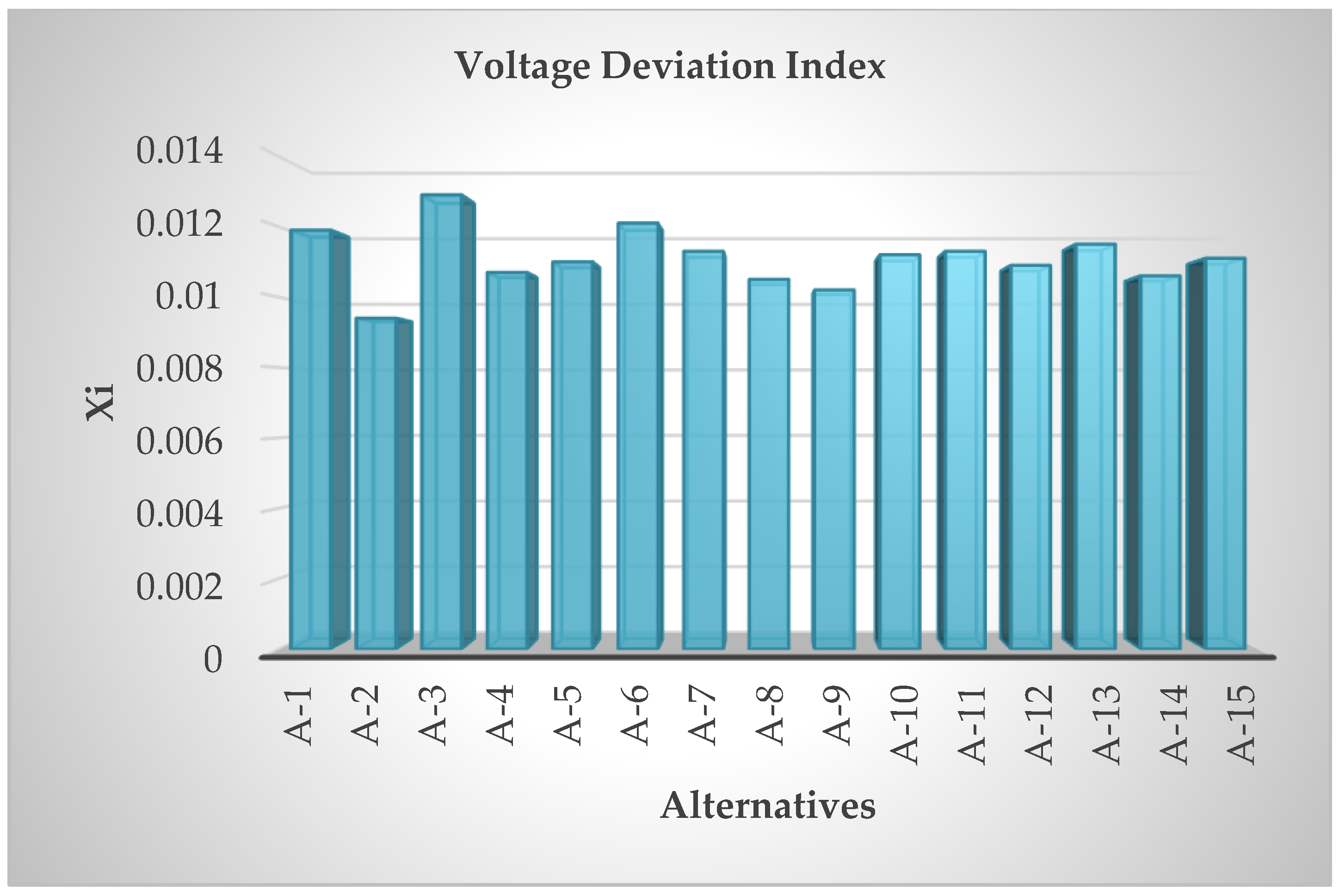
2.2.1. Voltage Deviation Index (X₁)

Voltage deviation index is one of the principal indices in operating any electric power system. It is determined as

$${X_1}_A=\{\begin{array}{ccccc}-\frac{\Delta V}{\Delta V_L}+1& & & & 0\le \Delta V\le \Delta V_L\\ \frac{\Delta V}{\Delta V_L}-1& & & & -\Delta V_L\le \Delta V<0\\ 0& & & & \Delta V_L<\Delta V<-\Delta V_L\end{array}forA=1,2,\dots ,N_a$$

(10)

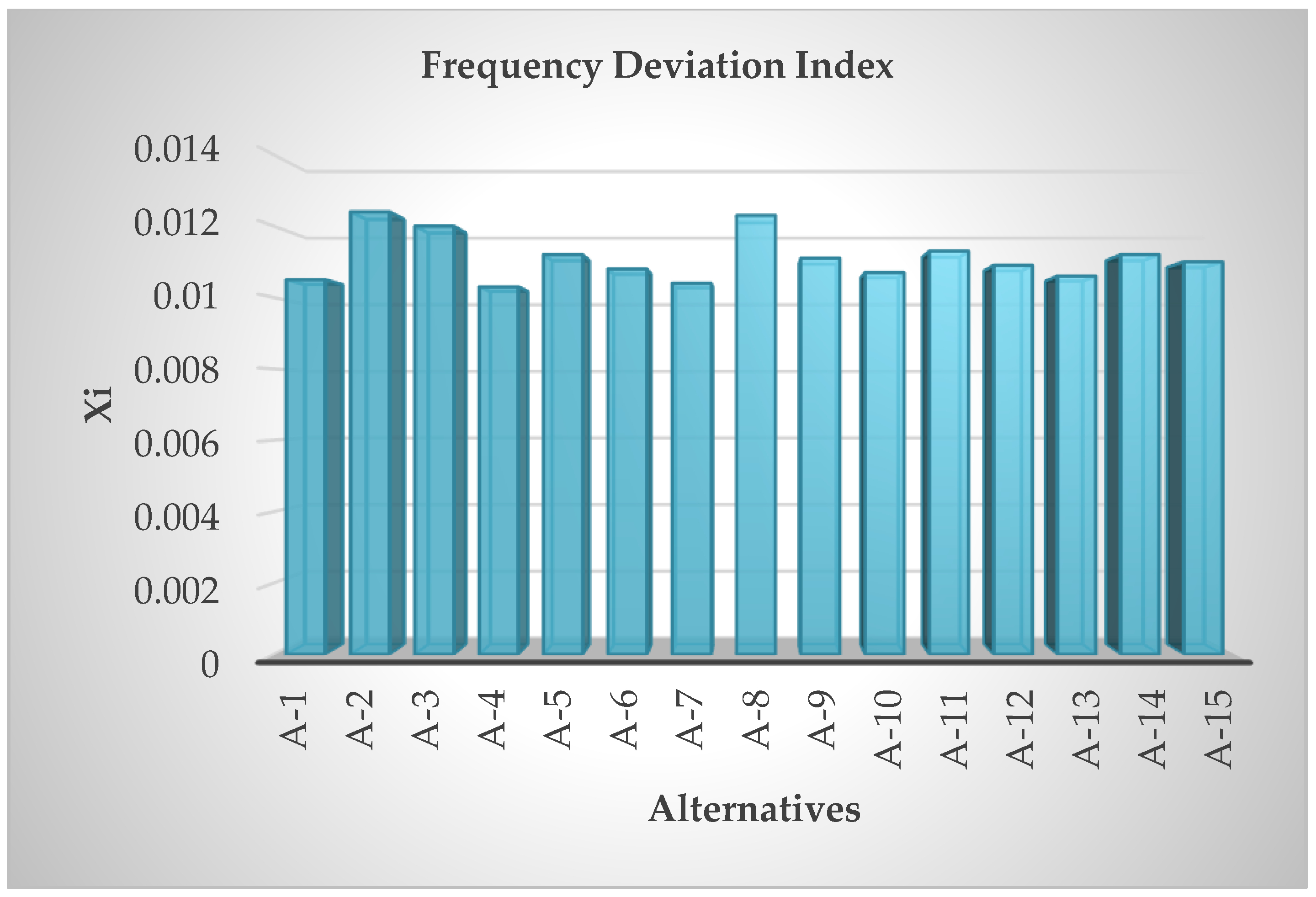
2.2.2. Frequency Deviation Index (X₂)

Frequency can be introduced as the backbone of the power quality. Frequency deviation index is calculated as follows:

$${X_2}_A=\{\begin{array}{ccccc}-\frac{\Delta F}{\Delta F_L}+1& & & & 0\le \Delta F\le \Delta F_L\\ \frac{\Delta F}{\Delta F_L}-1& & & & -\Delta F_L\le \Delta F<0\\ 0& & & & \Delta F_L<\Delta F<-\Delta F_L\end{array}forA=1,2,\dots ,N_a$$

(11)

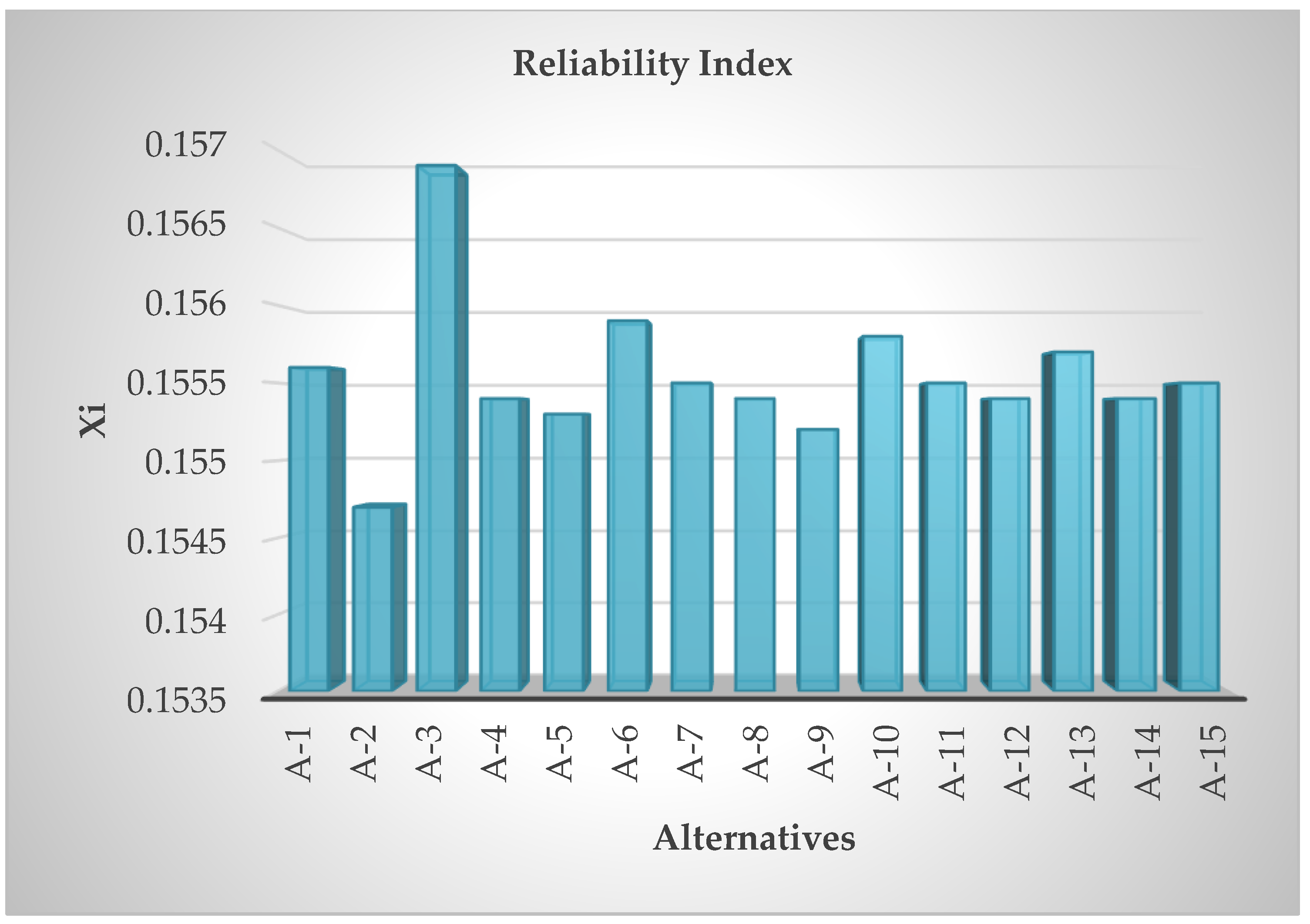
2.2.3. Reliability (X₃)

It is an indicator of customers’ interruptions and customer time lost for events lasting for more than three minutes as short interruptions are neglected [21]. It is the ability of the system to perform certain tasks under specific environmental conditions for a certain period of time. Any component failure in the electric distribution network causes interruptions to the customer services, like what happened in Ekpoma Network, Edo State, in Nigeria [30]. Interruptions are illustrated by many indicators such as System Average Interruption Frequency Index (SAIFI), Customer Average Interruption Duration Index (CAIDI), System Average Interruption Duration Index (SAIDI), Momentary Average Interruption Frequency Index (MAIFI) and Customer Total Average Interruption Duration Index (CTAIDI).

System Average Interruption Frequency Index (SAIFI) is a substantial indicator, which represents the total number of interrupted customers corresponding to the total number of all served customers during a specific period.

$$SAIFI=\frac{FrequencyofOutages}{Numberofcustomerssupplied}$$

(12)

$$X_{3_A}=1-{\sum }^{\text{}}(\frac{MG-i_{UP{C}_{Shareable}}\times SAIFI}{{\sum }^{\text{}}MG-i_{UP{C}_{Shareable}}})forA=1,2,\dots ,N_a$$

(13)

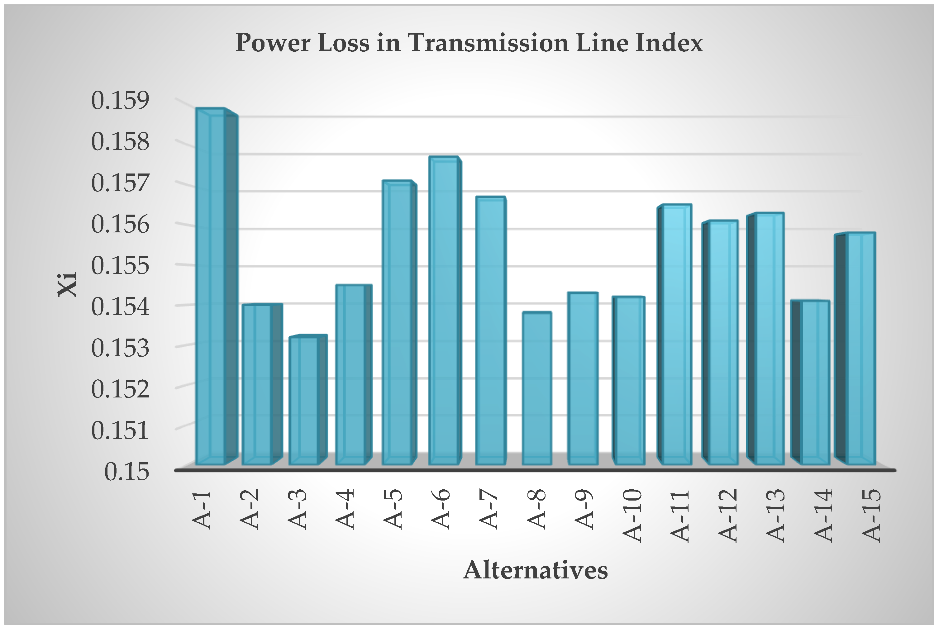
2.2.4. Power Loss in Transmission Lines Index (X₄)

Transmission Lines (T.L.) are the interconnecting lines between MGs, which facilitate the movement of electrical power. They are exposed to many losses, which affect the transmitting energy. Copper Loss is one of the main losses, which occur in transmission lines that depend on the length and the impedance of the line between the overloaded MG and the selected MG(s). It is presented as follows:

$$P_{Loss}=3\times {\left(\frac{PDL}{\surd 3\times V_L\times \cos \varnothing }\right)}^2\times Z_L\times L$$

(14)

$$X_{4_A}=1-{\sum }^{\text{}}(\frac{MG-i_{UP{C}_{Shareable}}\times P_{Loss}}{{\sum }^{\text{}}MG-i_{UP{C}_{Shareable}}})for\mathrm{A}=1,2,\dots ,N_a$$

(15)

where $P_{Loss}$ is the T.L. power loss (in kW). $Z_L$ is the impedance of transmission line per length, while L is the T.L. length $V_L$ is the line-to-line voltage (in V).

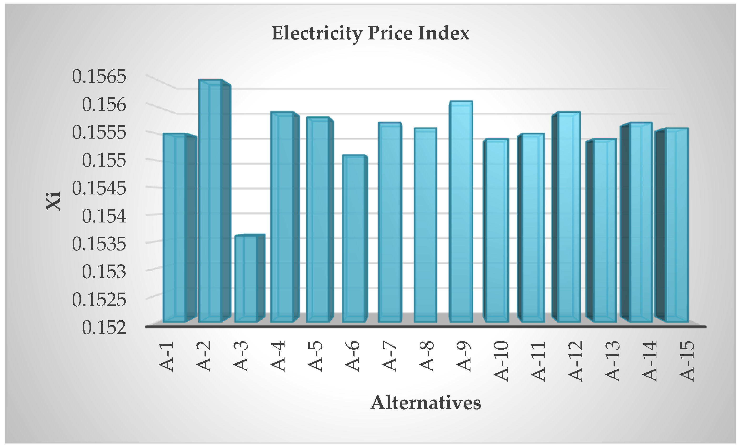
2.2.5. Electricity Price Index (X₅)

One of the main important criteria in selecting the best alternative is the Electricity Price (E.P. in $). As each MG has its own distributed generators, its owner can sell the electricity to the neighboring MG(s) for a different price. The difference in tariff is determined according to the variation of the peak hour and the usage of conventional fossil fuel resources. E.P. index is analysed as follows:

$$X_{5_A}=1-{\sum }^{\text{}}(\frac{MG-i_{UP{C}_{Shareable}}\times E.P}{{\sum }^{\text{}}MG-i_{UP{C}_{Shareable}}})for\mathrm{A}=1,2,\dots ,N_a$$

(16)

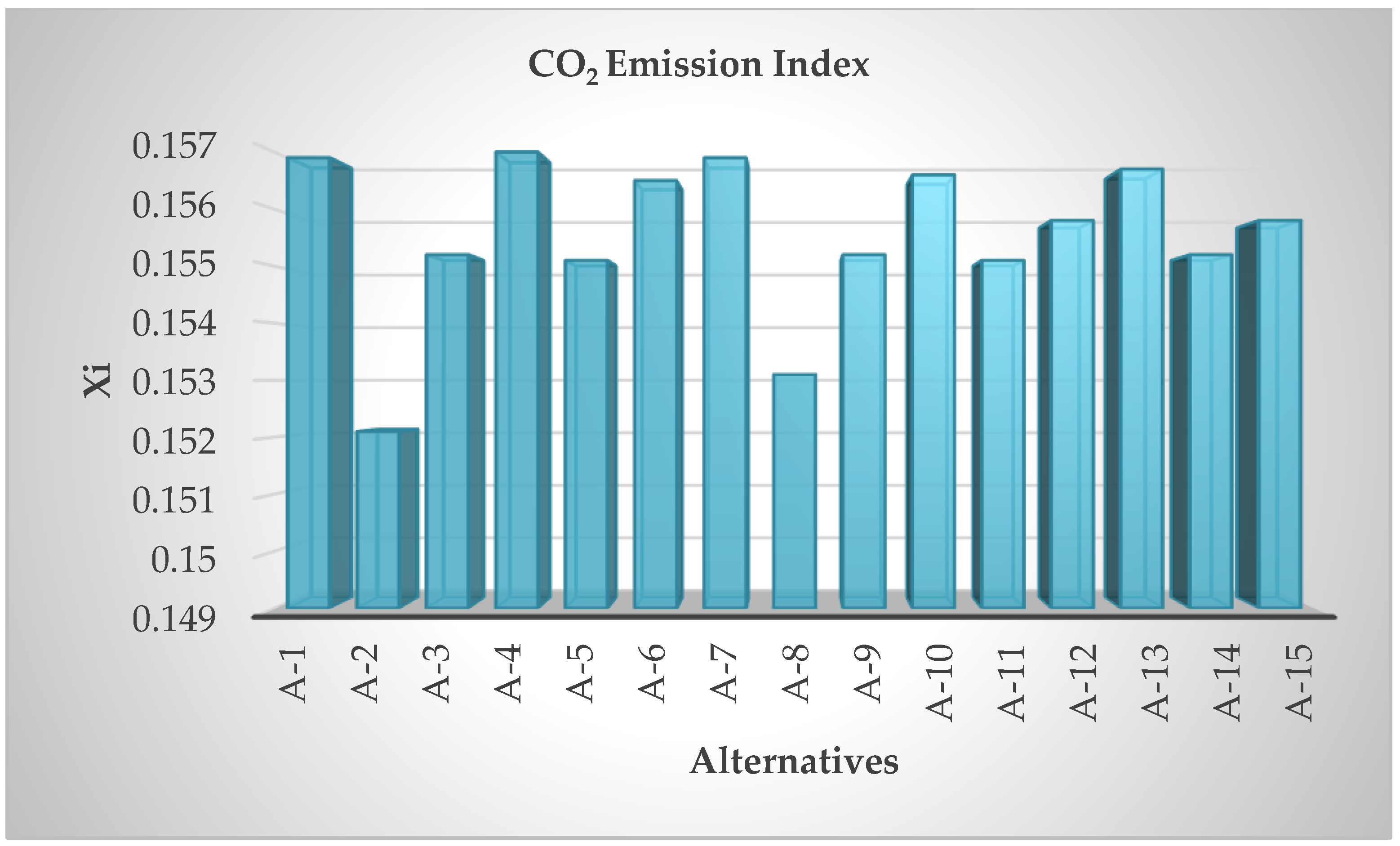
2.2.6. CO₂ Emission Index (X₆)

MGs have their own electrical energy generation resources. Each resource has different substantial effects on the environment. The network operator penalizes the MG owner according to the level of CO₂ emission resulting from the use of conventional fossil fuel resources. Less CO₂ emission means minimization of the penalties, which makes the alternative more desirable [31].

$$X_{6_A}=1-{\sum }^{\text{}}(\frac{MG-i_{UP{C}_{Shareable}}\times C{O}_{2}Emission}{{\sum }^{\text{}}MG-i_{UP{C}_{Shareable}}})for\mathrm{A}=1,2,\dots ,N_a$$

(17)

2.3. Decision-Making Criteria

The Decision-Making Criteria (DMC) depend on selecting the optimal alternative from a group of alternatives, considering a set of ($N_C)$ indices. Each index has a certain sharing weight supplementary to the others where ${\sum }_{j=1}^{N_C}{W}_j=1$. The matrix form of Decision-Making (DM) is expressed as follows:

$$\begin{array}{c}{A}_1\\ A_2\\ \begin{array}{c}⋮\\ A_{N_a}\end{array}\end{array}\left[\begin{array}{ccc}\begin{array}{c}\begin{array}{cc}{X}_{11}& X_{12}\end{array}\\ \begin{array}{cc}{X}_{11}& X_{22}\end{array}\end{array}& \cdots & \begin{array}{c}{X}_1{N}_c\\ X_2{N}_c\end{array}\\ ⋮& \ddots & ⋮\\ \begin{array}{cc}{X}_{N_{a1}}& X_{N_{a2}}\end{array}& \cdots & X_{N_a{N}_c}\end{array}\right]=\left[\begin{array}{c}{X}_1\\ X_2\\ \begin{array}{c}⋮\\ X_{N_a}\end{array}\end{array}\right]$$

(18)

Weighted Linear Normalization (WLN) is calculated for all the input data. It is used to rescale the values of the indices [32].

$$\begin{array}{c}{A}_1\\ A_2\\ \begin{array}{c}⋮\\ A_{N_a}\end{array}\end{array}\left[\begin{array}{ccc}\begin{array}{c}\begin{array}{cc}{W}_1{X}_{11}& W_2{X}_{12}\end{array}\\ \begin{array}{cc}{W}_2{X}_{11}& W_2{X}_{22}\end{array}\end{array}& \cdots & \begin{array}{c}{W}_{N_c}{X}_1{N}_c\\ W_{N_c}{X}_2{N}_c\end{array}\\ ⋮& \ddots & ⋮\\ \begin{array}{cc}{W}_1{X}_{N_{a1}}& W_2{X}_{N_{a2}}\end{array}& \cdots & W_{N_c}{X}_{N_a{N}_c}\end{array}\right]=\left[\begin{array}{c}{X}_1\\ X_2\\ \begin{array}{c}⋮\\ X_{N_a}\end{array}\end{array}\right]$$

(19)

Weighted Arithmetic Mean (WAM) is applied to the independent indices for decision-making. It evaluates the distinct importance of each index [32].

$$X_i=C_1\times C_2\times C_3\times C_4\times \frac{{\sum }_{i=1}^{N_c}{X}_i\times W_i}{6}$$

(20)

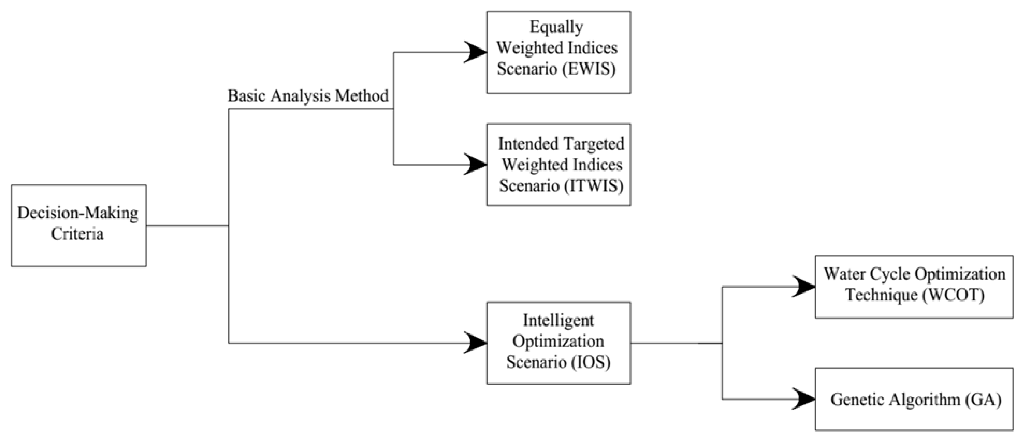
In this paper, the decision-making criteria is utilized by two main strategies as illustrated in Figure 3, which are affected by the sharing weights of the indices. The first strategy depends on Basic Analysis Methods (BAM) that are represented by the Equally Weighted Indices Scenario (EWIS) and the Intended Targeted Weighted Indices Scenario (ITWIS). The second strategy is the Intelligent Optimization Scenario (IOS) based on the Water Cycle Optimization Technique (WCOT). WCOT results are compared with Genetic Algorithm (GA).

3. The Intelligent Optimization Scenario (IOS)

3.1. The Water Cycle Optimization Technique (WCOT)

The Water Cycle Optimization Technique (WCOT) is inspired by the water cycle process phenomenon and is developed by Hadi Eskander et al. [26]. It is mainly based on the flow of rivers and streams into the sea. Over decades, various algorithms were used to solve optimization problems, which guaranteed obtaining the global optimal solution for the studied system. Recently, researchers have tended to use meta-heuristic algorithms based on natural inspiration. The algorithms combine the rules and randomness of the natural phenomena [33].

The WCA depends on an initial population called raindrops. The best raindrop is assumed to be the sea, then the river, then the streams which flow into the river and the sea [26].

The WCOT procedures are discussed below.

3.1.1. Population Initialization

In this stage, random values for the system variables are assigned, within the problem space, to be the initial raindrops (RD) Population (P_RD). The raindrop is represented as an array 1× N_vars

$$RD=\left[\begin{array}{ccc}{X}_1& X_2& \begin{array}{cc}\dots & X_N\end{array}\end{array}\right]$$

(21)

$$P_{RD}=\left[\begin{array}{c}RD1\\ RD2\\ \begin{array}{c}⋮\\ RD{N}_P\end{array}\end{array}\right]=\left[\begin{array}{ccc}\begin{array}{ccc}\begin{array}{c}{X}_1^1\\ X_1^2\end{array}& \begin{array}{c}{X}_2^1\\ X_2^2\end{array}& \begin{array}{c}{X}_3^1\\ X_3^2\end{array}\end{array}& \cdots & \begin{array}{c}{X}_{N_{var}}^1\\ X_{N_{var}}^2\end{array}\\ ⋮& \ddots & ⋮\\ \begin{array}{ccc}{X}_1^{N_P}& X_2^{N_P}& X_3^{N_P}\end{array}& \cdots & X_{N_{vars}}^{N_P}\end{array}\right]$$

(22)

where N_vars is the number of variables. N_P is the Number of Raindrops (initial population).

The evaluating fitness function (FF) can be expressed as follows:

$$F{F}_i=f\left(X_1^i,X_2^i,\dots ,X_{N_{vars}}^i\right),i=1,2,\dots ,N_P$$

(23)

All rivers and streams end up in the sea, which represents the optimum solution. The raindrops form the streams, which flow directly into the sea, or the river then the sea. This can be represented as follows:

$$N_{SR}=NumberofRivers+1$$

(24)

$$N_{RD}=N_P-N_{SR}$$

(25)

where N_SR is the number of the rivers and the sea (the number of the rivers in addition to the sea).

The number of streams ($N{S}_n$) which flow into the specific rivers or the sea are expressed as follows:

$$N{S}_n=round\left\{\left|\frac{F{F}_n}{{\sum }_{i=1}^{N_{SR}}F{F}_n}\right|\times N_{RD}\right\},n=1,2,\dots ,N_{SR}$$

(26)

Streams flow into the rivers or the sea through a distance (d) as illustrated in Figure 4, and Equation (27).

$$X\in \left(0,C\times d\right),C>1$$

(27)

where C is between 1 and 2. The detected best value of C is 2. The distance X varies always between 0 and (C × d).

If the FF given by the stream is better than its connecting river, the positions of the river and the stream should be exchanged. In addition, such exchange may happen between the river and the sea as shown in Figure 5.

The new positions of the river and the stream are as follows:

$$X_{stream}^{i+1}=X_{stream}^i+rand\times C\times \left(X_{River}^i-X_{stream}^i\right)$$

(28)

$$X_{River}^{i+1}=X_{River}^i+rand\times C\times \left(X_{Sea}^i-X_{River}^i\right)$$

(29)

3.1.2. The Evaporation Process

Evaporation is an important factor for preventing rapid convergence. To avoid trapping in local optima, the water of the sea evaporates as rivers and streams flow into the sea. The river flowing into the sea is determined by Equation (30)

$$\left|X_{sea}^i-X_{River}^i\right|<d_{max}$$

(30)

where i = 1, 2, …, N_SR-1. D_max is a number close to zero. If the distance between the river and the sea is less than d_max, it means that the sea and the river can join each other naturally. After sufficient evaporation, the precipitation process commences. On the other side, the search intensity near the sea is reduced, as the distance is greater than d_max. In general, d_max mainly controls the intensity search near the sea which represents the optimum solution and it can be decreased by:

$$d_{max}^{i+1}=d_{max}^i-\frac{d_{max}^i}{ma{x}_{iteration}}$$

(31)

3.1.3. The Raining Process

This process is applied after the evaporation condition is fulfilled and satisfied. In this stage, the raindrops form streams in the different locations, which flow into the river or directly into the sea. The new location of the formed streams which only directly flow into the sea is expressed as follows:

$$X_{stream}^{new}=LB+rand\times \left(UB-LB\right)$$

(32)

where LB and UB are the lower and upper bounds, respectively. The optimum solution of the streams which directly flow into the sea is explored as follows:

$$X_{stream}^{new}=X_{sea}+\surd \mu \times \mathrm{randn}\left(1,N_{vars}\right)$$

(33)

where $\sqrt{\mu }$ represents the standard deviation, as µ is the variance coefficient which depends on the searching region within a range around the sea. The small value µ indicates that the algorithm searches in a small region. For a suitable region, µ is set to be 0.1.

3.1.4. Convergence Criteria

In WCOT, the optimization process progresses until the convergence criteria (termination condition) are achieved.

The Water Cycle Optimization Technique Algorithm is explained by the flowchart in Figure 6. The WCOT flowchart explains each step from the initial population until the convergence criteria.

3.2. Genetic Algorithm

In this paper, a comparison is held between the Water Cycle Optimization Technique (WCOT) and the Genetic Algorithm (GA). The topology of the Genetic Algorithm is based on the biological evolution process of computational data and the mechanism of natural genetics selection [34,35]. GA is composed of three main significant operators, which are reproduction, crossover and mutation. These operators result in an optimum solution using a fitness function, as it maps the natural objective function.

Both WCOT and GA are utilized to produce the optimal weighted solution for each alternative as a step in the decision-making algorithm program. The weighted arithmetic mean is the objective function (fitness function) to find the global optimum for the decision-making.

The flowchart of the main outlines of decision-making criteria, starting with calculating the UPC_actual for all MGs to check if interconnection is required or not, is displayed in Figure 7. If any MG is flagged as an overloaded MG, the operation conditional flag (IOS problem constraints) must be calculated for each other MG to check the validity of interconnection with the overloaded MG. The optimum solution for supplying the overloaded MG is based on the weights of indices. The weights of indices are studied by three scenarios, which are the Equally Weighted Indices Scenario (EWIS), the Intended Targeted Weighted Indices Scenario (ITWIS) and the Intelligent Optimization Scenario (IOS) based on the Water Cycle Optimization Technique (WCOT) and the Genetic Algorithm (GA). A command signal is sent to the relevant interconnecting switch (ISS) to be closed.

4. Hybrid MG Integration Simulation and Results

In the proposed system under study, the distribution network consists of 5 isolated Micro- MG(s). At normal operation, each micro-grid supplies its own load with its own distributed resources. The distributed network is fully controlled using a continuous global controller. The global controller checks if any MG(s) has/have any deficiency. The global controller detects deficiency by comparing the obtained data from measurement with the data in

Table 1. Data of the distributed network under Study.

Micro-Grid	Load Power (kW)	Generated Power (kW)	SAIFI	Electricity Price ($)	CO2 Emission ($/ton of CO2)	∆V	∆F
MG-1	12	73	5.18	0.2867	2.312	0.0108	0.003304
MG-2	72	54	3.6	0.2869	4.307	0	0
MG-3	35	76	5.62	0.2608	3.437	0.0192	0.002104
MG-4	48	74	4.59	0.3328	2.697	0.0073	0.002338
MG-5	20	81	5.27	0.2752	2.277	0.0147	0.003438

. Table 1 represents 6 indices; load power-generated power, reliability factor, SAIFI, CO₂ emission, voltage deviation, and frequency deviation for each MG. In

Table 2. Assumed data of transmission lines between Micro-Grids (MGs).

Sending MG	Receiving MG	Length (km)	Resistive Impedance (Ohm/km)
MG-1	MG-2	10	0.131
MG-1	MG-3	14	0.119
MG-1	MG-4	15	0.147
MG-1	MG-5	12	0.172
MG-2	MG-3	18	0.119
MG-2	MG-4	11.5	0.198
MG-2	MG-5	9	0.23
MG-3	MG-4	12.5	0.172
MG-3	MG-5	16	0.119
MG-4	MG-5	16.5	0.119

, the data related to the transmission lines between all MG(s) are presented.

Table 2 shows that the five MGs have a closed range along the transmission lines (km) and impedances (Ohm/km) as power is transmitted in a medium voltage range with 66 kV. In addition, Table 1 declares that MG-2 will be flagged as an overloaded MG corresponding to Equation (2), because load (72 kW) is greater than generation (54 kW) in MG-2. MG-2 cannot supply its own load by itself under normal conditions. The supply of overloaded MG can be done by one of fifteen alternatives, each of which has six indices with six different weights. To sum up the six indices which are relating to the six different indices, the indices have to be first normalized. Each alternative has its own topology, so a linear normalization is determined for each alternative. Linear normalization has been done to select the optimum alternative with respect to the other alternatives as in

Table 3. The linear normalization matrix.

Alternative	Participating Micro-Grid	∆V	∆F	SAIFI	Power Loss	Electricity Price	CO2 Emission
A-1	{MG-1}	0.0714	0.0630	0.9338	0.9536	0.9328	0.9412
A-2	{MG-3}	0.0561	0.0743	0.9282	0.9242	0.9388	0.9126
A-3	{MG-4}	0.0778	0.0721	0.9414	0.9194	0.9219	0.9314
A-4	{MG-5}	0.0643	0.0618	0.9327	0.9267	0.9355	0.9421
A-5	{MG-1, MG-3}	0.0658	0.0672	0.9318	0.9428	0.9350	0.9307
A-6	{MG-1, MG-4}	0.0728	0.0650	0.9355	0.9461	0.9304	0.9390
A-7	{MG-1, MG-5}	0.0679	0.0624	0.9333	0.9403	0.9341	0.9416
A-8	{MG-3, MG-4}	0.0632	0.0736	0.9325	0.9226	0.9333	0.9187
A-9	{MG-3, MG-5}	0.0612	0.0665	0.9310	0.9258	0.9367	0.9311
A-10	{MG-4, MG-5}	0.0673	0.0641	0.9346	0.9251	0.9324	0.9397
A-11	{MG-1, MG-3, MG-4}	0.0676	0.0679	0.9332	0.9393	0.9330	0.9308
A-12	{MG-1, MG-3, MG-5}	0.0652	0.0651	0.9321	0.9367	0.9352	0.9350
A-13	{MG-1, MG-4, MG-5}	0.0691	0.0636	0.9343	0.9377	0.9326	0.9404
A-14	{MG-3, MG-4, MG-5}	0.0638	0.0673	0.9326	0.9248	0.9345	0.9311
A-15	{MG-1, MG-3, MG-4, MG-5}	0.0665	0.0658	0.9330	0.9350	0.9339	0.9347

.

Operational Conditional flags (IOS problem constraints) should be studied for all MGs. MG-4 is flagged to show that the shareable unused power capacity does not satisfy its own load after taking into account the safety margin as in Equation (3). MG-4 cannot supply the overloaded MG by itself but it can share a specific power with any neighboring MG to supply the overloaded one.

4.1. Basic Analysis Methods

The basic analysis methods are divided into two scenarios. The first scenario is the Equally Weighted Indices Scenario (EWIS). The second scenario is the Intended Targeted Weighted Indices Scenario (ITWIS).

4.1.1. The Equally Weighted Indices Scenario (EWIS)

The first scenario assumes that all indices are equally weighted which means that W₁ = W₂ = W₃ = W₄ = W₅ = W₆ = 0.16667. All indices have been studied for each alternative as represented in Figure 8, Figure 9, Figure 10, Figure 11, Figure 12 and Figure 13, based on the results of

Table A1. The equally weighted arithmetic mean decision-making matrix for different aggregators.

Alter-natives	Participating Micro-Grid	C1	C2	C3	C4	X1	X2	X3	X4	X5	X6	Xi
A-1	{MG-1}	1	1	1	1	0.0119	0.0105	0.1556	0.1589	0.1555	0.1569	0.1082
A-2	{MG-3}	1	1	1	1	0.0094	0.0124	0.1547	0.1540	0.1565	0.1521	0.1065
A-3	{MG-4}	1	0	1	1	0.0129	0.0120	0.1569	0.1532	0.1536	0.1552	0
A-4	{MG-5}	1	1	1	1	0.0107	0.0103	0.1554	0.1545	0.1559	0.1570	0.1073
A-5	{MG-1, MG-3}	1	1	1	1	0.0110	0.0112	0.1553	0.1571	0.1558	0.1551	0.1076
A-6	{MG-1, MG-4}	1	1	1	1	0.0121	0.0108	0.1559	0.1577	0.1551	0.1565	0.1080
A-7	{MG-1, MG-5}	1	1	1	1	0.0113	0.0104	0.1555	0.1567	0.1557	0.1569	0.1078
A-8	{MG-3, MG-4}	1	1	1	1	0.0105	0.0123	0.1554	0.1538	0.1556	0.1531	0.1068
A-9	{MG-3, MG-5}	1	1	1	1	0.0102	0.0111	0.1552	0.1543	0.1561	0.1552	0.1070
A-10	{MG-4, MG-5}	1	1	1	1	0.0112	0.0107	0.1558	0.1542	0.1554	0.1566	0.1073
A-11	{MG-1, MG-3, MG-4}	1	1	1	1	0.0113	0.0113	0.1555	0.1565	0.1555	0.1551	0.1076
A-12	{MG-1, MG-3, MG-5}	1	1	1	1	0.0109	0.0109	0.1554	0.1561	0.1559	0.1558	0.1075
A-13	{MG-1, MG-4, MG-5}	1	1	1	1	0.0115	0.0106	0.1557	0.1563	0.1554	0.1567	0.1077
A-14	{MG-3, MG-4, MG-5}	1	1	1	1	0.0106	0.0112	0.1554	0.1541	0.1557	0.1552	0.1071
A-15	{MG-1, MG-3, MG-4, MG-5}	1	1	1	1	0.0111	0.0110	0.1555	0.1558	0.1556	0.1558	0.1075

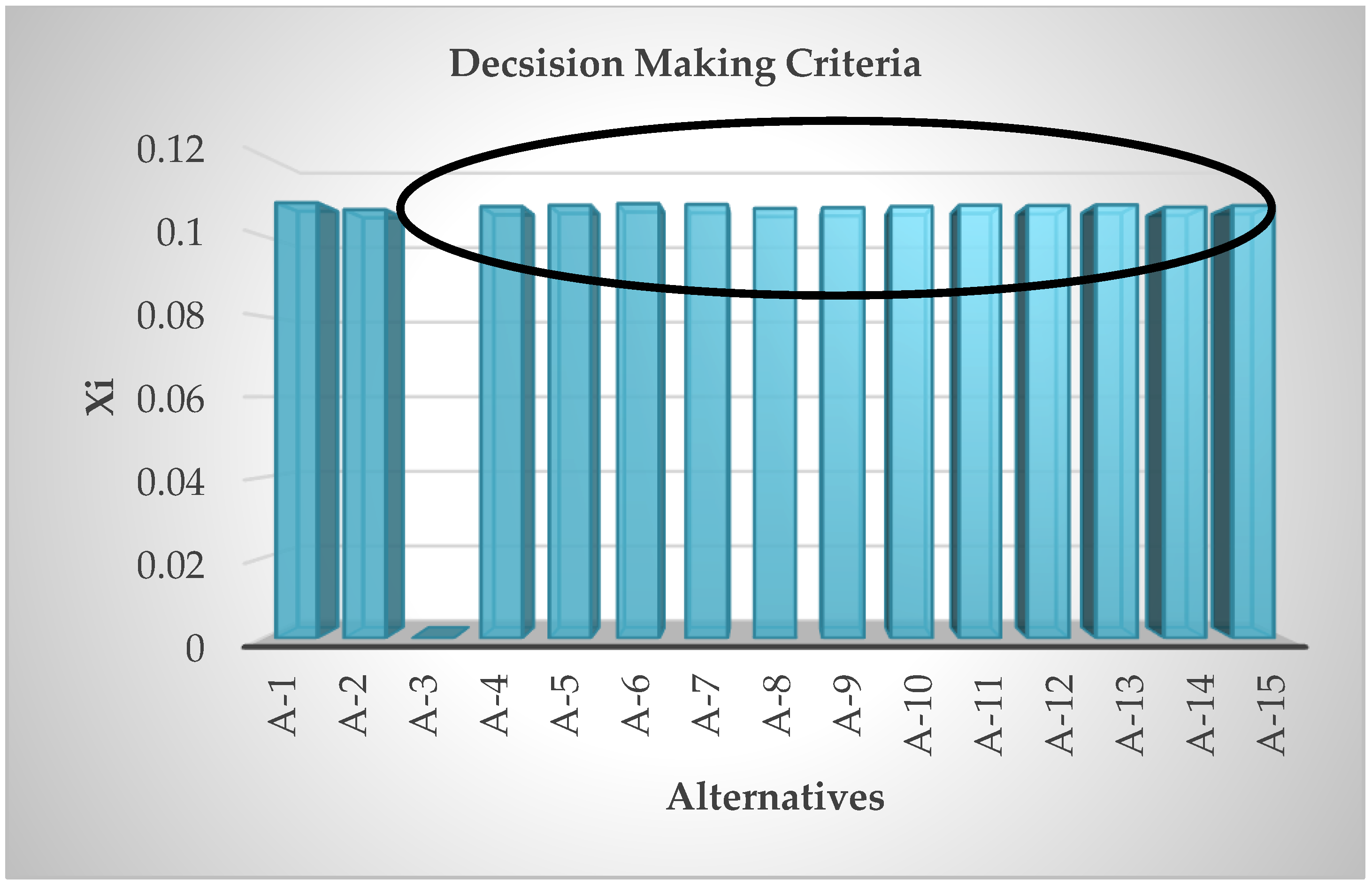
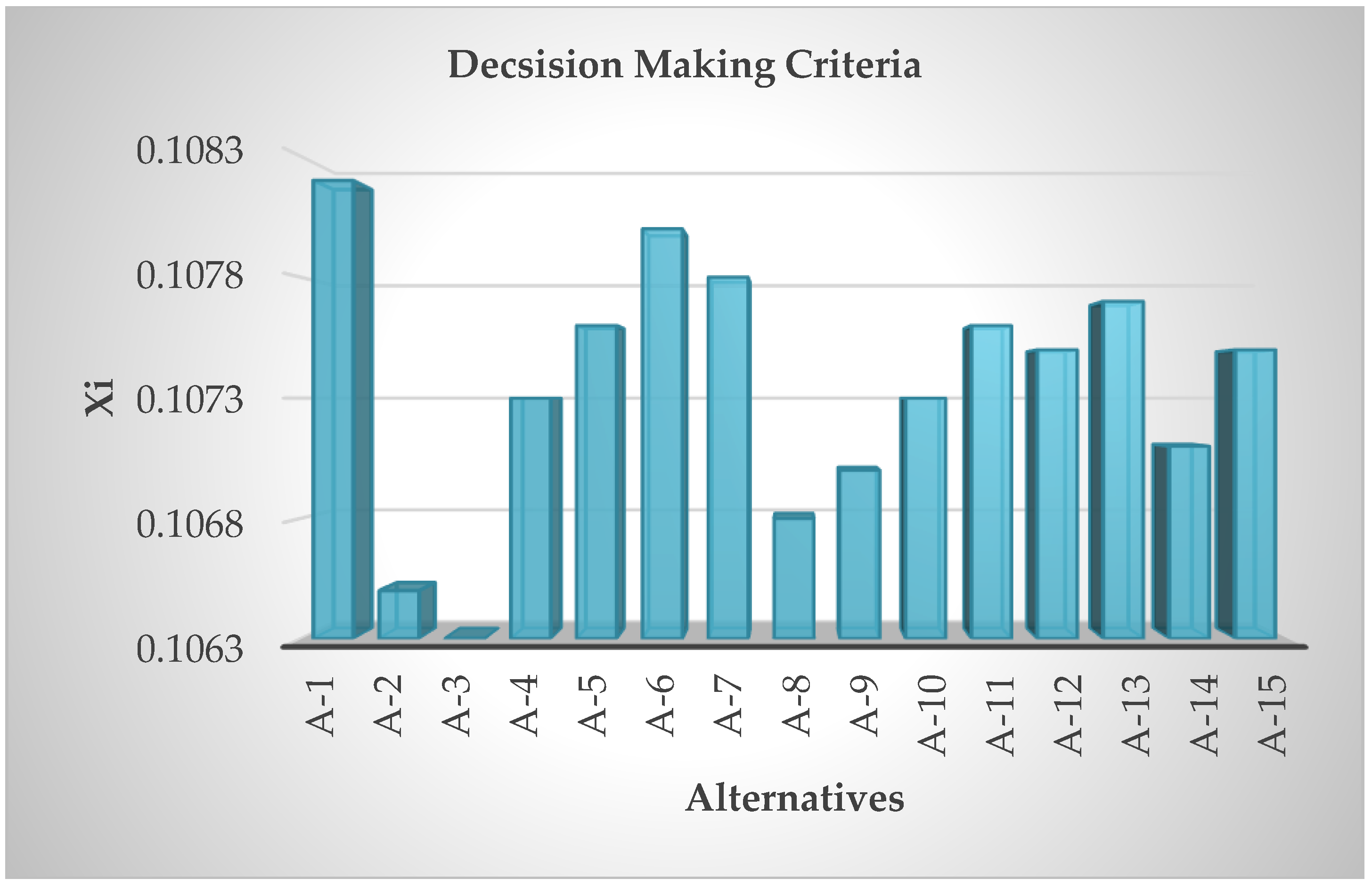
(Appendix). Each index has its own optimum solution alternative which differs from one index to another. Decision-making criteria are studied to merge all indices to have the optimum alternative as in Equation (20) and represented in Figure 14. Figure 15 is the zoomed version of Figure 14, (by making the reference 0.1063). The decision algorithm is flagged to show that MG-1 (1st alternative) is the optimum solution for all the indices compared with the other alternatives.

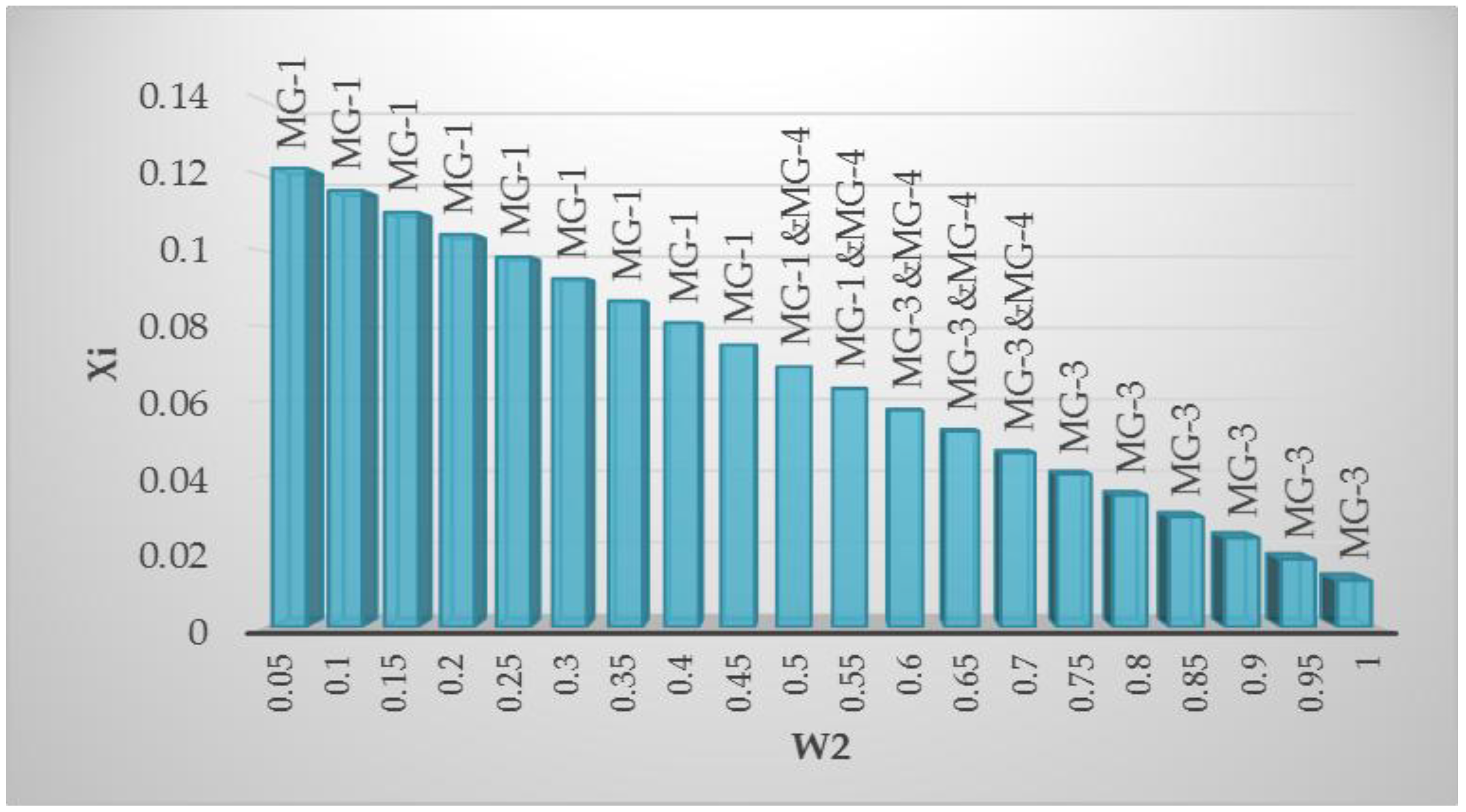
4.1.2. The Intended Targeted Weighted Indices Scenario (ITWIS)

The second scenario is based on changing the weight of only one index and making all the remaining indices equal in weight. If W is the weight of 1st index, then the weights for all the remaining indices will be ($\frac{\mathbf{1}-\mathit{W}}{\mathbf{5}}$). It is concluded that if the increasing or decreasing of the chosen indices exceeds a specific limit, the decision-making of optimum alternative differs from one index to another as represented in Figure 16, Figure 17 and Figure 18.

Table A2. Biased weighted index of frequency deviation, reliability and power loss in transmission line indices.

The Changeable Weighting	W1	W2	W3	W4	W5	W6	Xi	Decision-Making
W2	0	1	0	0	0	0	0.0124	MG-3
	0.01	0.95	0.01	0.01	0.01	0.01	0.018	MG-3
	0.02	0.9	0.02	0.02	0.02	0.02	0.0237	MG-3
	0.03	0.85	0.03	0.03	0.03	0.03	0.0293	MG-3
	0.04	0.8	0.04	0.04	0.04	0.04	0.035	MG-3
	0.05	0.75	0.05	0.05	0.05	0.05	0.0406	MG-3
	0.06	0.7	0.06	0.06	0.06	0.06	0.0463	MG-3 & MG-4
	0.07	0.65	0.07	0.07	0.07	0.07	0.052	MG-3 & MG-4
	0.08	0.6	0.08	0.08	0.08	0.08	0.0576	MG-3 & MG-4
	0.09	0.55	0.09	0.09	0.09	0.09	0.0633	MG-1 & MG-4
	0.1	0.5	0.1	0.1	0.1	0.1	0.0692	MG-1 & MG-4
	0.11	0.45	0.11	0.11	0.11	0.11	0.075	MG-1
	0.12	0.4	0.12	0.12	0.12	0.12	0.0809	MG-1
	0.13	0.35	0.13	0.13	0.13	0.13	0.0867	MG-1
	0.14	0.3	0.14	0.14	0.14	0.14	0.0926	MG-1
	0.15	0.25	0.15	0.15	0.15	0.15	0.0984	MG-1
	0.16	0.2	0.16	0.16	0.16	0.16	0.1043	MG-1
	0.17	0.15	0.17	0.17	0.17	0.17	0.1102	MG-1
	0.18	0.1	0.18	0.18	0.18	0.18	0.116	MG-1
	0.19	0.05	0.19	0.19	0.19	0.19	0.1219	MG-1
W3	0	0	1	0	0	0	0.1559	MG-1 & MG-4
	0.01	0.01	0.95	0.01	0.01	0.01	0.153	MG-1 & MG-4
	0.02	0.02	0.9	0.02	0.02	0.02	0.1502	MG-1 & MG-4
	0.03	0.03	0.85	0.03	0.03	0.03	0.1473	MG-1 & MG-4
	0.04	0.04	0.8	0.04	0.04	0.04	0.1444	MG-1 & MG-4
	0.05	0.05	0.75	0.05	0.05	0.05	0.1415	MG-1 & MG-4
	0.06	0.06	0.7	0.06	0.06	0.06	0.1387	MG-1 & MG-4
	0.07	0.07	0.65	0.07	0.07	0.07	0.1358	MG-1 & MG-4
	0.08	0.08	0.6	0.08	0.08	0.08	0.1329	MG-1 & MG-4
	0.09	0.09	0.55	0.09	0.09	0.09	0.1301	MG-1 & MG-4
	0.1	0.1	0.5	0.1	0.1	0.1	0.1272	MG-1
	0.11	0.11	0.45	0.11	0.11	0.11	0.1243	MG-1
	0.12	0.12	0.4	0.12	0.12	0.12	0.1215	MG-1
	0.13	0.13	0.35	0.13	0.13	0.13	0.1187	MG-1
	0.14	0.14	0.3	0.14	0.14	0.14	0.1158	MG-1
	0.15	0.15	0.25	0.15	0.15	0.15	0.113	MG-1
	0.16	0.16	0.2	0.16	0.16	0.16	0.1101	MG-1
	0.17	0.17	0.15	0.17	0.17	0.17	0.1073	MG-1
	0.18	0.18	0.1	0.18	0.18	0.18	0.1044	MG-1
	0.19	0.19	0.05	0.19	0.19	0.19	0.1016	MG-1
W4	0	0	0	1	0	0	0.1589	MG-1
	0.01	0.01	0.01	0.95	0.01	0.01	0.1559	MG-1
	0.02	0.02	0.02	0.9	0.02	0.02	0.1528	MG-1
	0.03	0.03	0.03	0.85	0.03	0.03	0.1498	MG-1
	0.04	0.04	0.04	0.8	0.04	0.04	0.1468	MG-1
	0.05	0.05	0.05	0.75	0.05	0.05	0.1437	MG-1
	0.06	0.06	0.06	0.7	0.06	0.06	0.1407	MG-1
	0.07	0.07	0.07	0.65	0.07	0.07	0.1376	MG-1
	0.08	0.08	0.08	0.6	0.08	0.08	0.1346	MG-1
	0.09	0.09	0.09	0.55	0.09	0.09	0.1315	MG-1
	0.1	0.1	0.1	0.5	0.1	0.1	0.1285	MG-1
	0.11	0.11	0.11	0.45	0.11	0.11	0.1255	MG-1
	0.12	0.12	0.12	0.4	0.12	0.12	0.1224	MG-1
	0.13	0.13	0.13	0.35	0.13	0.13	0.1194	MG-1
	0.14	0.14	0.14	0.3	0.14	0.14	0.1163	MG-1
	0.15	0.15	0.15	0.25	0.15	0.15	0.1133	MG-1
	0.16	0.16	0.16	0.2	0.16	0.16	0.1102	MG-1
	0.17	0.17	0.17	0.15	0.17	0.17	0.1072	MG-1
	0.18	0.18	0.18	0.1	0.18	0.18	0.1042	MG-1
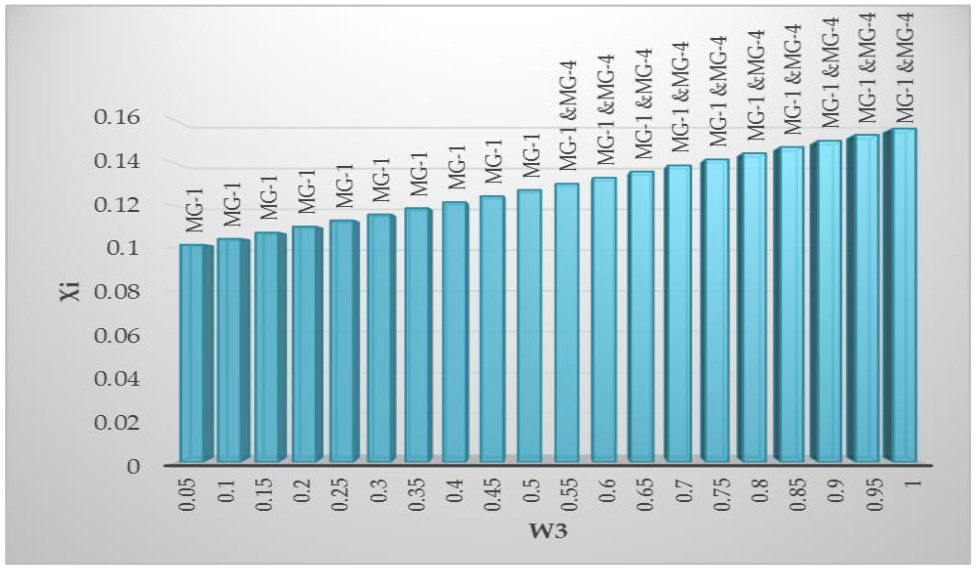
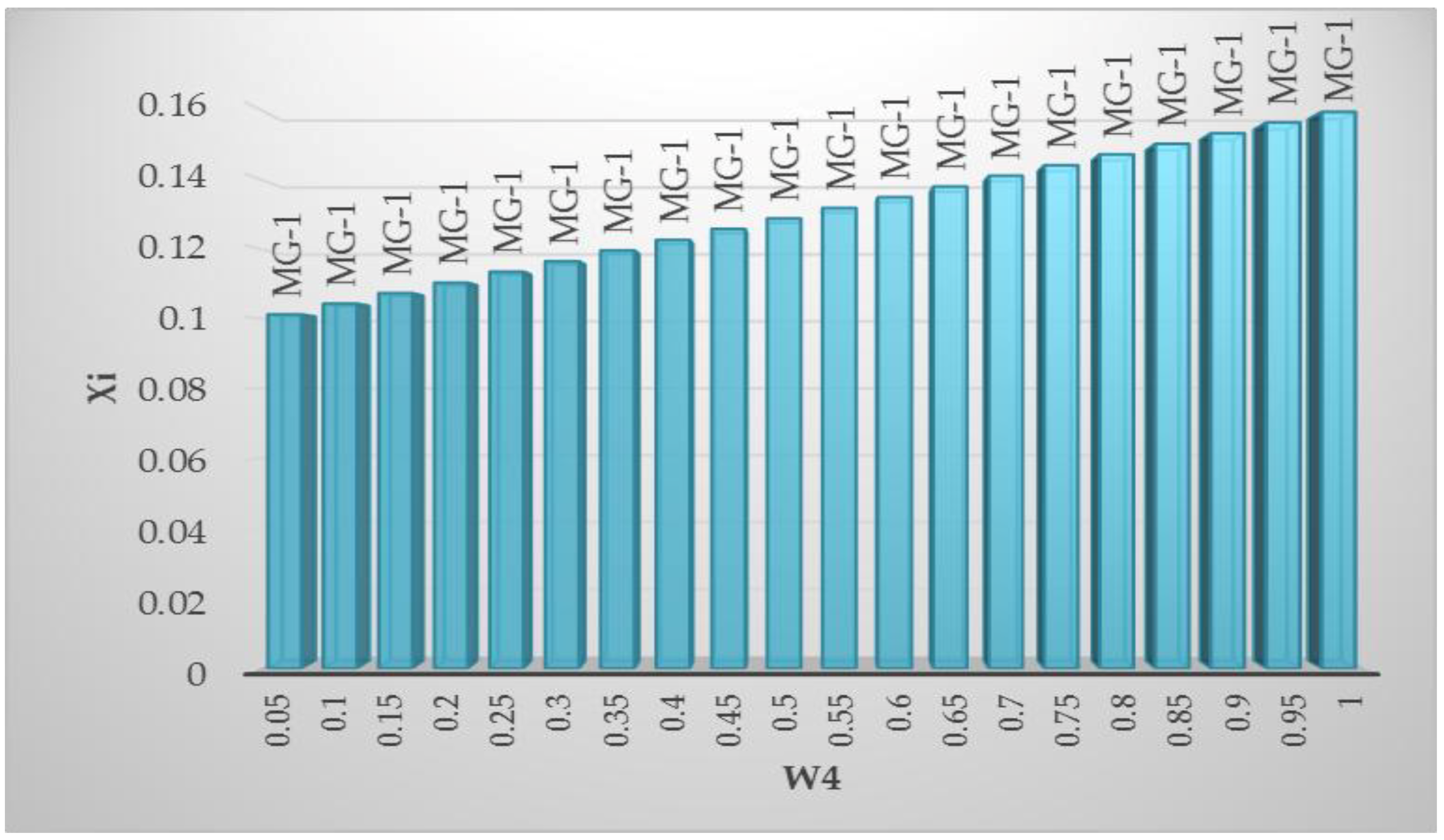
	0.19	0.19	0.19	0.05	0.19	0.19	0.1011	MG-1

(in Appendix) illustrates the data of Figure 16, Figure 17 and Figure 18, in which the weights (W) of the frequency deviation, reliability and transmission line power loss indices are changed gradually from 0.05 to 1. The corresponding weighted arithmetic mean (X_i) is calculated to determine the optimal selected alternative for the decision-making step. The variation effect of the weights of voltage deviation, electricity price and CO₂ emission indices on the optimal decision-making is explained in

Table A3. Biased weighted index of voltage deviation, electricity price and CO₂ emission indices.

The Changeable Weighting	W1	W2	W3	W4	W5	W6	Xi	Decision-Making
W1	1	0	0	0	0	0	0.0121	MG-1 & MG-4
	0.95	0.01	0.01	0.01	0.01	0.01	0.0179	MG-1 & MG-4
	0.9	0.02	0.02	0.02	0.02	0.02	0.0236	MG-1 & MG-4
	0.85	0.03	0.03	0.03	0.03	0.03	0.0294	MG-1 & MG-4
	0.8	0.04	0.04	0.04	0.04	0.04	0.0351	MG-1 & MG-4
	0.75	0.05	0.05	0.05	0.05	0.05	0.0409	MG-1 & MG-4
	0.7	0.06	0.06	0.06	0.06	0.06	0.0467	MG-1 & MG-4
	0.65	0.07	0.07	0.07	0.07	0.07	0.0524	MG-1 & MG-4
	0.6	0.08	0.08	0.08	0.08	0.08	0.0582	MG-1 & MG-4
	0.55	0.09	0.09	0.09	0.09	0.09	0.0639	MG-1 & MG-4
	0.5	0.1	0.1	0.1	0.1	0.1	0.0697	MG-1
	0.45	0.11	0.11	0.11	0.11	0.11	0.0755	MG-1
	0.4	0.12	0.12	0.12	0.12	0.12	0.0812	MG-1
	0.35	0.13	0.13	0.13	0.13	0.13	0.087	MG-1
	0.3	0.14	0.14	0.14	0.14	0.14	0.0928	MG-1
	0.25	0.15	0.15	0.15	0.15	0.15	0.0986	MG-1
	0.2	0.16	0.16	0.16	0.16	0.16	0.1044	MG-1
	0.15	0.17	0.17	0.17	0.17	0.17	0.1101	MG-1
	0.1	0.18	0.18	0.18	0.18	0.18	0.1159	MG-1
	0.05	0.19	0.19	0.19	0.19	0.19	0.1217	MG-1
W5	0	0	0	0	1	0	0.1565	MG-3
	0.01	0.01	0.01	0.01	0.95	0.01	0.1535	MG-3
	0.02	0.02	0.02	0.02	0.9	0.02	0.1505	MG-3
	0.03	0.03	0.03	0.03	0.85	0.03	0.1475	MG-3
	0.04	0.04	0.04	0.04	0.8	0.04	0.1445	MG-3
	0.05	0.05	0.05	0.05	0.75	0.05	0.1415	MG-3
	0.06	0.06	0.06	0.06	0.7	0.06	0.1385	MG-3
	0.07	0.07	0.07	0.07	0.65	0.07	0.1356	MG-1
	0.08	0.08	0.08	0.08	0.6	0.08	0.1328	MG-1
	0.09	0.09	0.09	0.09	0.55	0.09	0.1299	MG-1
	0.1	0.1	0.1	0.1	0.5	0.1	0.1271	MG-1
	0.11	0.11	0.11	0.11	0.45	0.11	0.1243	MG-1
	0.12	0.12	0.12	0.12	0.4	0.12	0.1214	MG-1
	0.13	0.13	0.13	0.13	0.35	0.13	0.1186	MG-1
	0.14	0.14	0.14	0.14	0.3	0.14	0.1158	MG-1
	0.15	0.15	0.15	0.15	0.25	0.15	0.1129	MG-1
	0.16	0.16	0.16	0.16	0.2	0.16	0.1101	MG-1
	0.17	0.17	0.17	0.17	0.15	0.17	0.1073	MG-1
	0.18	0.18	0.18	0.18	0.1	0.18	0.1044	MG-1
	0.19	0.19	0.19	0.19	0.05	0.19	0.1016	MG-1
W6	0	0	0	0	0	1	0.157	MG-5
	0.01	0.01	0.01	0.01	0.01	0.95	0.154	MG-5
	0.02	0.02	0.02	0.02	0.02	0.9	0.151	MG-5
	0.03	0.03	0.03	0.03	0.03	0.85	0.1481	MG-1
	0.04	0.04	0.04	0.04	0.04	0.8	0.1452	MG-1
	0.05	0.05	0.05	0.05	0.05	0.75	0.1423	MG-1
	0.06	0.06	0.06	0.06	0.06	0.7	0.1394	MG-1
	0.07	0.07	0.07	0.07	0.07	0.65	0.1364	MG-1
	0.08	0.08	0.08	0.08	0.08	0.6	0.1335	MG-1
	0.09	0.09	0.09	0.09	0.09	0.55	0.1306	MG-1
	0.1	0.1	0.1	0.1	0.1	0.5	0.1277	MG-1
	0.11	0.11	0.11	0.11	0.11	0.45	0.1248	MG-1
	0.12	0.12	0.12	0.12	0.12	0.4	0.1218	MG-1
	0.13	0.13	0.13	0.13	0.13	0.35	0.1189	MG-1
	0.14	0.14	0.14	0.14	0.14	0.3	0.116	MG-1
	0.15	0.15	0.15	0.15	0.15	0.25	0.1131	MG-1
	0.16	0.16	0.16	0.16	0.16	0.2	0.1102	MG-1
	0.17	0.17	0.17	0.17	0.17	0.15	0.1072	MG-1
	0.18	0.18	0.18	0.18	0.18	0.1	0.1043	MG-1
	0.19	0.19	0.19	0.19	0.19	0.05	0.1014	MG-1

(Appendix).

It is observed that due to the close distribution between the MGs and the closeness of transmission lines and their impedances, all results tend to MG-1 as shown in Figure 18. As shown in Table A2 and Table A3 (Appendix), variation in the weight of the indices below the validation border 0.05 for each index (limits violation case) may lead to different decision-making, with better results than the WCOT and GA. The results show that some indices are excluded by taking a lower weight corresponding to the other indices.

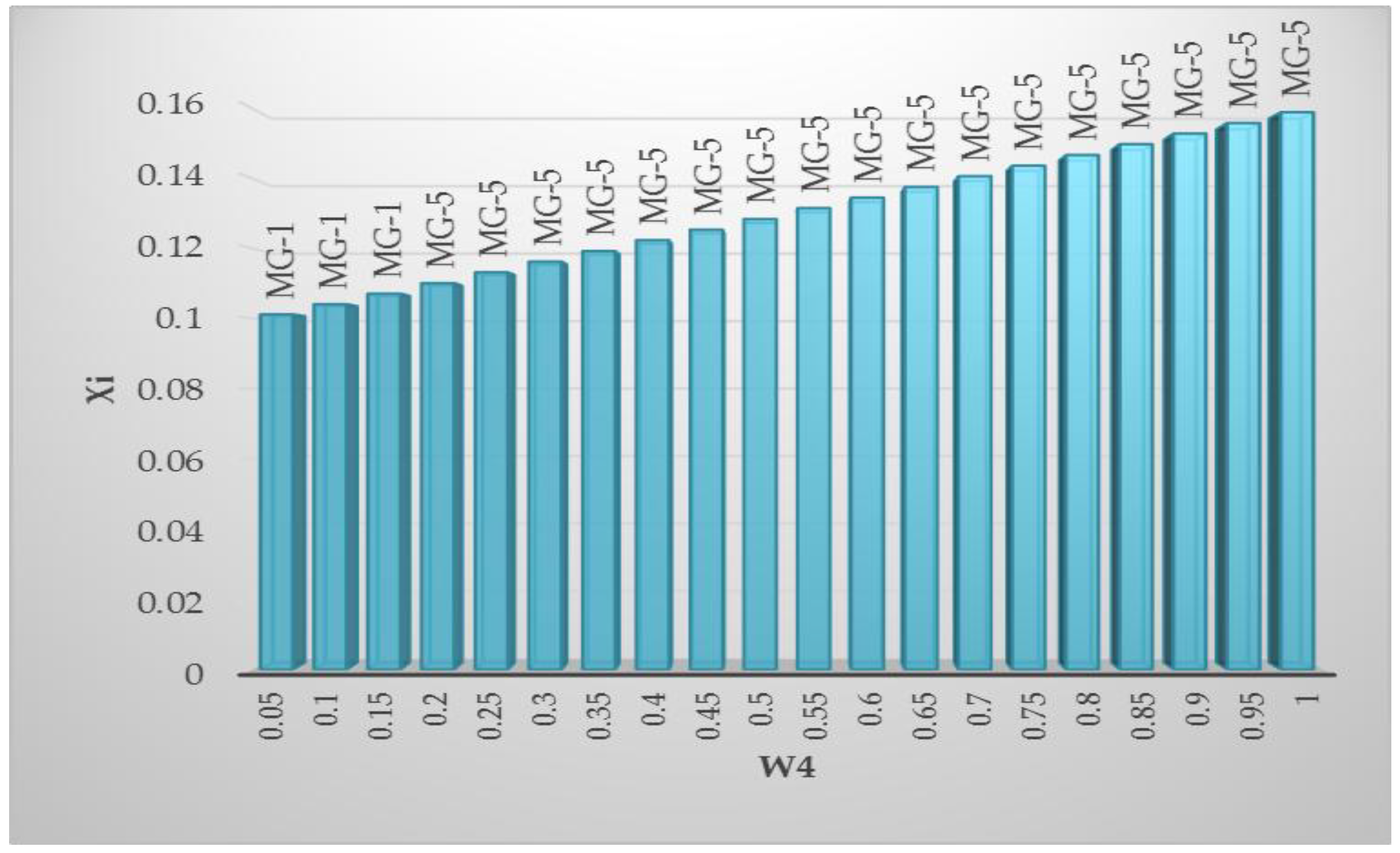
To check the effect of the intermediate linking between the optimal selected alternative, and transmission lines and their impedances, a change is executed on the transmission line lengths and impedances between MGs. The impedance of transmission line between the overloaded Micro-Grid (MG-2) and (MG-5) is reduced to 0.13 Ohm/km instead of 0.23 Ohm/km as shown in

Table 4. Different assumed data of transmission lines between MG-5 and MG-2.

Sending and Receiving MG		Length (km)	Impedance (Ohm/km)
MG-1	MG-2	10	0.131
MG-1	MG-3	14	0.119
MG-1	MG-4	15	0.147
MG-1	MG-5	12	0.172
MG-2	MG-3	18	0.119
MG-2	MG-4	11.5	0.198
MG-2	MG-5	9	0.13
MG-3	MG-4	12.5	0.172
MG-3	MG-5	16	0.119
MG-4	MG-5	16.5	0.119

. The relatively smallest impedance is between MG-5 and MG-2, which affects the transmission power losses indices. The optimal decision-making is modified as shown in Figure 19, as explained in

Table A4. Biased weighted index of power loss in transmission line index for the modified transmission lines between MG-2 and MG-5.

The Changeable Weighting	W1	W2	W3	W4	W5	W6	Xi	Decision-Making
W4	0	0	0	1	0	0	0.1586	MG-5
	0.01	0.01	0.01	0.95	0.01	0.01	0.1555	MG-5
	0.02	0.02	0.02	0.9	0.02	0.02	0.1525	MG-5
	0.03	0.03	0.03	0.85	0.03	0.03	0.1495	MG-5
	0.04	0.04	0.04	0.8	0.04	0.04	0.1464	MG-5
	0.05	0.05	0.05	0.75	0.05	0.05	0.1434	MG-5
	0.06	0.06	0.06	0.7	0.06	0.06	0.1404	MG-5
	0.07	0.07	0.07	0.65	0.07	0.07	0.1373	MG-5
	0.08	0.08	0.08	0.6	0.08	0.08	0.1343	MG-5
	0.09	0.09	0.09	0.55	0.09	0.09	0.1313	MG-5
	0.1	0.1	0.1	0.5	0.1	0.1	0.1282	MG-5
	0.11	0.11	0.11	0.45	0.11	0.11	0.1252	MG-5
	0.12	0.12	0.12	0.4	0.12	0.12	0.1222	MG-5
	0.13	0.13	0.13	0.35	0.13	0.13	0.1191	MG-5
	0.14	0.14	0.14	0.3	0.14	0.14	0.1161	MG-5
	0.15	0.15	0.15	0.25	0.15	0.15	0.1131	MG-5
	0.16	0.16	0.16	0.2	0.16	0.16	0.1100	MG-5
	0.17	0.17	0.17	0.15	0.17	0.17	0.1070	MG-1
	0.18	0.18	0.18	0.1	0.18	0.18	0.1040	MG-1
	0.19	0.19	0.19	0.05	0.19	0.19	0.1011	MG-1

(Appendix). MG-5, which has the smallest distance to the overloaded Micro-Grid (MG-2), is selected as the optimum solution.

4.1.3. The Intelligent Optimization Scenario (IOS) Results

The third scenario is obtained by applying the Water Cycle Optimization Technique (WCOT) and the results will be compared with the Genetic Algorithm (GA) as in

Table 5. Comparison between the Water Cycle Optimization Technique (WCOT) and the Genetic Algorithm (GA).

Alter-natives	The Water Cycle Optimization Technique (WCOT)						The Genetic Algorithm (GA)
	W1	W2	W3	W4	W5	W6	W1	W2	W3	W4	W5	W6
A-1	0.05	0.05	0.05	0.75	0.05	0.05	0.05	0.051	0.108	0.437	0.214	0.14
	Xi = 0.143720591235003						Xi = 0.142805874721561
A-2	0.05	0.05	0.05	0.05	0.75	0.05	0.05	0.05	0.363	0.071	0.38	0.087
	Xi = 0.141481999141277						Xi = 0.140824524050091
A-4	0.05	0.05	0.05	0.05	0.05	0.75	0.05	0.052	0.068	0.079	0.395	0.358
	Xi = 0.142101144475445						Xi = 0.141550396339045
A-5	0.05	0.05	0.05	0.75	0.05	0.05	0.05	0.05	0.057	0.232	0.523	0.088
	Xi = 0.142270253125611						Xi = 0.141622161729789
A-6	0.05	0.05	0.05	0.75	0.05	0.05	0.05	0.05	0.152	0.46	0.174	0.114
	Xi = 0.142789234327526						Xi = 0.142310973961454
A-7	0.05	0.05	0.05	0.05	0.05	0.75	0.05	0.05	0.061	0.205	0.168	0.466
	Xi = 0.142187199060368						Xi = 0.14204841360112
A-8	0.05	0.05	0.37	0.05	0.428	0.05	0.05	0.05	0.48	0.079	0.214	0.128
	Xi = 0.140876771116161						Xi = 0.140758932749476
A-9	0.05	0.05	0.05	0.05	0.75	0.05	0.05	0.05	0.177	0.191	0.217	0.316
	Xi = 0.141385440661611						Xi = 0.140870801351789
A-10	0.05	0.05	0.05	0.05	0.05	0.75	0.05	0.05	0.235	0.126	0.223	0.316
	Xi = 0.141824518391855						Xi = 0.141341251241211
A-11	0.05	0.05	0.05	0.75	0.05	0.05	0.05	0.05	0.198	0.281	0.252	0.17
	Xi = 0.141847517552339						Xi = 0.141422981153506
A-12	0.05	0.05	0.05	0.75	0.05	0.05	0.05	0.051	0.137	0.326	0.255	0.182
	Xi = 0.14152247144387						Xi = 0.141411738939702
A-13	0.05	0.05	0.05	0.05	0.05	0.75	0.05	0.05	0.057	0.399	0.076	0.368
	Xi = 0.142022681231797						Xi = 0.141900352891222
A-14	0.05	0.05	0.187	0.05	0.453	0.211	0.05	0.051	0.379	0.06	0.39	0.07
	Xi = 0.141005201014154						Xi = 0.14106635566993
A-15	0.05	0.05	0.05	0.708	0.091	0.05	0.05	0.05	0.135	0.219	0.201	0.345
	Xi = 0.141311119272574						Xi = 0.141346001161916

. The operation conditional flags are considered to be the artificial intelligent algorithm constraints. The WCOT and GA are operated for each alternative. It is observed that the optimum solution calculated from the WCOT is better than GA as the optimum solution in Table 5.

From these Tables, the results reveal the need for the optimization technique to find the optimal solution due to the complexity of the targeted variables and the small applied range. The Water Cycle Optimization Technique (WCOT) shows the power over the GA and the heuristic techniques in the first and second scenarios. The only value that indicates maximum objective function (optimal solution) than the WCOT was obtained by violating the lower constraints.

5. Conclusions

This paper presents an optimal, efficient, reliable, economical and eco-friendly power sharing solution in case of overloaded or insufficient power generation in a hybrid micro-grid, through its integration with other neighboring micro-grids. The optimal selection is built on one of the three studied scenarios, which are based on the weighted arithmetic mean of the six multi-objective indices and the four operation conditional flags. The six indices are voltage deviation, frequency deviation, reliability, power loss in transmission lines, electricity price and CO₂ emissions, respectively. The first scenario module is the basic Equally Weighted Indices Scenario (EWIS), through which the effect of each index on the optimum combination is studied. The second scenario, which is called the Intended Targeted Weighted Indices Scenario (ITWIS), studies the optimal combination based on maximizing the effect of one of the indices over the others through its sharing weight. It progresses through step changing the weight of the selected index while keeping all the other indices equally weighted. The third scenario is the Intelligent Optimization Scenario (IOS). It utilizes the Water Cycling Optimization Technique (WCOT) to assign the global optimal MG integration with its six indices optimum sharing weights. The WCOT selections are compared with the Genetic Algorithm (GA) optimal solutions. The studied modules are applied to a distribution power network, which consists of five hybrid MGs, with one overloaded MG. The results indicate the optimal technical, economical and environment friendly MGs integration. It is observed that the optimum solution, which satisfies the minimum risk value for each index and indicates the highest fitness function value, is determined by the WCOT. From the obtained results, it is concluded that for all indices, and consequently their weights, the cost function is not sensitive to their variation within a certain limit of the individual index. When this limit is exceeded, the optimal decision may be reconsidered.