Sensorless Direct Torque Control of Surface-Mounted Permanent Magnet Synchronous Motors with Nonlinear Kalman Filtering

Abstract

The demand for sensorless control of surface-mounted permanent magnet synchronous motor drives has grown rapidly. Among various sensorless control techniques developed, Matsui’s current model-based approach and the extended Kalman filter approach have gained much attention. However, the performance of these control methods can be severely worsened or may even become unstable under strong disturbances or sensing failures. This paper presents a comparative study of the extended Kalman filter, the resilient extended Kalman filter, and the unscented Kalman filter-based sensorless direct torque and flux control approaches for the surface-mounted permanent magnet synchronous motor drives. Computer simulation studies and hardware implementation results have shown the efficiency and superior performance of the resilient extended Kalman filter and the unscented Kalman filter over the traditional extended Kalman filter for sensorless direct torque control applications.

1. Introduction

Over the past decades, there has been a rapid increase in the deployment of surface-mounted permanent magnet synchronous motors (SPMSM) in industrial and commercial applications, such as wind energy conversion systems, hybrid electric vehicles, robotics, home appliances, etc. Adjustable speed SPM drives offer many distinct advantages including large torque to weight ratio, wide constant-power operating range, high efficiency and reliability, etc.

A wide variety of adjustable-speed control techniques have been studied in literature for permanent magnet AC motors. Among them, field oriented control (FOC) for SPMSM drives has reached industrial application maturity. FOC requires coordinate transforms and space-vector pulse width modulation (SVPWM), through which the flux and torque of AC machines are controlled independently [1,2,3,4,5]. In order to eliminate these requirements, direct torque control (DTC) was proposed as a powerful alternative [6,7]. The advantages of DTC include fast dynamic responses, elimination of coordinate transforms and SVPWM. DTC also has minor disadvantages, in comparison with FOC, including: difficulties to control torque and flux at relatively low speed, variable switching frequency, larger harmonics, larger noise level and ripples at low speed range. Despite the aforementioned shortcomings, DTC is also a feasible solution for commercial permanent magnet AC drives.

DTC is in nature “sensorless”, as rotor position is not required for performing coordinate transform [6,7]. However, it relies on the information of stator flux vector. Especially, at relatively low speed range, due to inaccurate estimation of flux vector, DTC suffers from the performance degradation. Sensorless estimation of stator flux and rotor speed has to be designed to preserve the advantages of direct torque control. For traditional DTC, stator flux linkage (${\lambda }_s$) is estimated through integrating stator induced voltage over time.

$${\lambda }_s\left(t\right)=\int (v_s-R_s{i}_s)dt+{\lambda }_s\left(0\right)$$

(1)

Even minor dc offsets in voltage or current signals accumulated by integration will form a substantial disturbance. Hence, traditional estimation of ${\lambda }_s$ contains large and noisy ripples [8,9,10].

To improve the estimation of stator flux linkage, various estimators have been developed including the back-emf integration methods such as low-pass filtering [11,12,13], and stabilizing the integrator with a PI-corrector or current offset methods [14,15,16,17]. However, these approaches are not designed for real-time estimation. The sliding mode observer (SMO) is developed for providing real-time state estimates for permanent magnet synchronous motors in [18,19,20]. However, higher-order derivatives presented in SMO are not desirable for hardware implementations. The extended Kalman filter (EKF) is a popular approach for sensorless control scheme. However, the performance of EKF deteriorates or may even become unstable under measurement failure conditions [21,22,23,24,25,26,27].

To improve EKF performance under external disturbances, noise and measurement failures, this paper presents a comparative study of the extended Kalman filter (EKF), the resilient extended Kalman filter (REKF), and the unscented Kalman filter (UKF)-based sensorless direct torque control approaches for SPMSM drives. Computer simulation studies and hardware implementation results have shown the efficiency and superior performance of the resilient extended Kalman filter and the unscented Kalman filter over the traditional extended Kalman filter for sensorless direct torque control applications.

This paper is organized as follows: Section 2 presents the dynamics of surface-mounted permanent magnet synchronous motors. Section 3 provides the overall control scheme of direct torque control. Section 4 presents the traditional extended Kalman filtering, the resilient extended Kalman filter and the unscented Kalman filter for nonlinear estimation. Computer simulation results and hardware implementation results are illustrated in Section 5. Finally, conclusions are summarized in Section 6.

2. Dynamics of Surface-Mounted Permanent Magnet Synchronous Motors

Applying Park’s transform, the surface-mounted permanent magnet synchronous motors (SPMSM) can be modeled as follows:

$$\begin{array}{cc}\hfill v_d& =R_s{i}_d+\frac{d{\lambda }_d}{dt}-{\omega }_e{\lambda }_q\hfill \end{array}$$

(2)

$$\begin{array}{cc}\hfill v_q& =R_s{i}_q+\frac{d{\lambda }_q}{dt}+{\omega }_e{\lambda }_d\hfill \end{array}$$

(3)

$$\begin{array}{cc}\hfill {\lambda }_d& =L_s{i}_d+{\lambda }_m\hfill \end{array}$$

(4)

$$\begin{array}{cc}\hfill {\lambda }_q& =L_s{i}_q\hfill \end{array}$$

(5)

It should be noted that the direct and quadrature axis stator inductance are the same for SPMSM, i.e., $L_d=L_q=L_s$, as no rotor saliency exists.

Equivalently, the current frame of reference model can be reached as follows:

$$\begin{array}{cc}\hfill \frac{d{i}_d}{dt}& =-\frac{R_s}{L_s}{i}_d+{\omega }_e{i}_q+\frac{1}{L_s}{v}_d\hfill \end{array}$$

(6)

$$\begin{array}{cc}\hfill \frac{d{i}_q}{dt}& =-\frac{R_s}{L_s}{i}_q-{\omega }_e{i}_d-{\omega }_e\frac{{\lambda }_m}{L_s}+\frac{1}{L_s}{v}_q\hfill \end{array}$$

(7)

The developed electromechanical torque is

$$\begin{array}{cc}\hfill {\tau }_e& =\frac{3}{2}\frac{P}{2}{\lambda }_m{i}_q\hfill \end{array}$$

(8)

Note that the mechanical and electrical angular velocities are related by

$$\begin{array}{cc}\hfill {\omega }_e& =\frac{P}{2}{\omega }_m\hfill \end{array}$$

(9)

The mechanical dynamics can be summarized as

$$\begin{array}{cc}\hfill \frac{d{\omega }_m}{dt}& =\frac{1}{J}({\tau }_e-{\tau }_l-D{\omega }_m)\hfill \end{array}$$

(10)

Applying (8) and (9), we have

$$\begin{array}{cc}\hfill \frac{d{\omega }_e}{dt}& =\frac{3}{2J}{\left(\frac{P}{2}\right)}^2{\lambda }_m{i}_q-\frac{P}{2J}{\tau }_l-\frac{D}{J}{\omega }_e,\hfill \end{array}$$

(11)

and

$$\begin{array}{cc}\hfill 1-1\frac{d{\theta }_e}{dt}& ={\omega }_e\hfill \end{array}$$

(12)

The external torque load ${\tau }_l$ is also considered as state variable, which is assumed to be constant over a brief period of sampling time $T_s$, i.e., we have

$$\begin{array}{cc}\hfill \frac{d{\tau }_l}{dt}& \approx 0\hfill \end{array}$$

(13)

The continuous-time SPMSM state space model can be written as follows:

$$\begin{array}{c}\hfill \dot{x}=\frac{d}{dt}\left[\begin{array}{c}{i}_d\\ i_q\\ {\omega }_e\\ {\theta }_e\\ {\tau }_l\end{array}\right];x=\left[\begin{array}{c}{i}_d\\ i_q\\ {\omega }_e\\ {\theta }_e\\ {\tau }_l\end{array}\right];u=\left[\begin{array}{c}{v}_d\\ v_q\end{array}\right];y=\left[\begin{array}{c}{i}_d\\ i_q\end{array}\right]\end{array}$$

(14)

$$\begin{array}{ccc}\hfill \dot{x}& =& A_c\left(x\right)+B_c\left(u\right)=f(x,u)\hfill \end{array}$$

(15)

$$\begin{array}{ccc}\hfill y& =& h_c\left(x\right)=h(x,u),\hfill \end{array}$$

(16)

where we have

$$\begin{array}{c}\hfill A_c=\left[\begin{array}{ccccc}-\frac{R_s}{L_s}& {\omega }_e& 0& 0& 0\\ -{\omega }_e& -\frac{R_s}{L_s}& -\frac{{\lambda }_m}{L_s}& 0& 0\\ 0& \beta {\lambda }_m& -\frac{D}{J}& 0& -\frac{P}{2J}\\ 0& 0& 1& 0& 0\\ 0& 0& 0& 0& 0\end{array}\right];B_c=\left[\begin{array}{cc}\frac{1}{L_s}& 0\\ 0& \frac{1}{L_s}\\ 0& 0\\ 0& 0\\ 0& 0\end{array}\right];h_c=\left[\begin{array}{ccccc}1& 0& 0& 0& 0\\ 0& 1& 0& 0& 0\end{array}\right]\end{array}$$

(17)

and

$$\begin{array}{c}\hfill \beta =\frac{3}{2J}{\left(\frac{P}{2}\right)}^2\end{array}$$

(18)

Notice that subscript c represents continuous-time signals.

Applying Euler’s discretization, the discrete-time system model can be reached as follows:

$$\begin{array}{cc}\hfill x_{k+1}=& x_k+T_{s}f(x_k,u_k)\hfill \\ \hfill y_k=& h(x_k,u_k)\hfill \end{array}$$

(19)

where $T_s$ is the sampling time.

Based on Jacobian matrices computation, a linear-time-invariant discrete-time state space model can be reached as follows:

$${\widehat{x}}_{k+1}=\left[\begin{array}{c}{i}_{d\left({\widehat{x}}_{k+1}\right)}\\ i_{q\left({\widehat{x}}_{k+1}\right)}\\ {\omega }_{e\left({\widehat{x}}_{k+1}\right)}\\ {\theta }_{e\left({\widehat{x}}_{k+1}\right)}\\ {\tau }_{l\left({\widehat{x}}_{k+1}\right)}\end{array}\right]=A_k\left[\begin{array}{c}{i}_{d\left({\widehat{x}}_k\right)}\\ i_{q\left({\widehat{x}}_k\right)}\\ {\omega }_{e\left({\widehat{x}}_k\right)}\\ {\theta }_{e\left({\widehat{x}}_k\right)}\\ {\tau }_{l\left({\widehat{x}}_k\right)}\end{array}\right]+B_k\left[\begin{array}{c}{v}_{d\left({\widehat{x}}_k\right)}\\ v_{q\left({\widehat{x}}_k\right)}\end{array}\right],$$

(20)

where we have

$$\begin{array}{cc}\hfill A_k& =I+{\left.\frac{\partial f(x_k,u_k)}{\partial x}\right|}_{x={\widehat{x}}_k}·T_s=\left[\begin{array}{ccccc}1-\frac{R_s}{L_s}{T}_s& {\omega }_e{T}_s& i_q{T}_s& 0& 0\\ -{\omega }_e{T}_s& 1-\frac{R_s}{L_s}{T}_s& -(i_d+\frac{{\lambda }_m}{L_s})T_s& 0& 0\\ 0& \beta {\lambda }_m{T}_s& 1-\frac{D}{J}{T}_s& 0& -\frac{P}{2J}{T}_s\\ 0& 0& T_s& 1& 0\\ 0& 0& 0& 0& 1\end{array}\right]\hfill \end{array}$$

(21)

Similarly,

$$\begin{array}{cc}\hfill B_k& ={\left.\frac{\partial f(x_k,u_k)}{\partial u}\right|}_{x={\widehat{x}}_k}·T_s=\left[\begin{array}{cc}\frac{T_s}{L_s}& 0\\ 0& \frac{T_s}{L_s}\\ 0& 0\\ 0& 0\\ 0& 0\end{array}\right]\hfill \end{array}$$

(22)

The measurement equation can be expressed as:

$$\begin{array}{cc}\hfill y_k& =h_k\left(x_k\right)=\left[\begin{array}{c}{i}_d\\ i_q\end{array}\right]=C_k\left[\begin{array}{c}{i}_d\\ i_q\\ {\omega }_e\\ {\theta }_e\\ {\tau }_l\end{array}\right],\hfill \end{array}$$

(23)

and

$$\begin{array}{cc}\hfill 1-1C_k& ={\left.\frac{\partial h\left(x_k\right)}{\partial x}\right|}_{x={\widehat{x}}_k}=\left[\begin{array}{ccccc}1& 0& 0& 0& 0\\ 0& 1& 0& 0& 0\end{array}\right]\hfill \end{array}$$

(24)

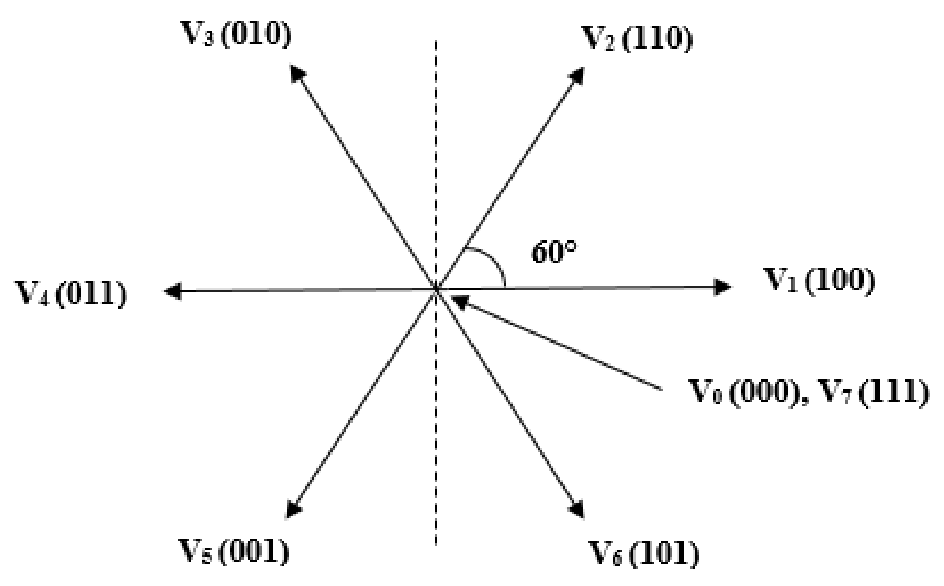
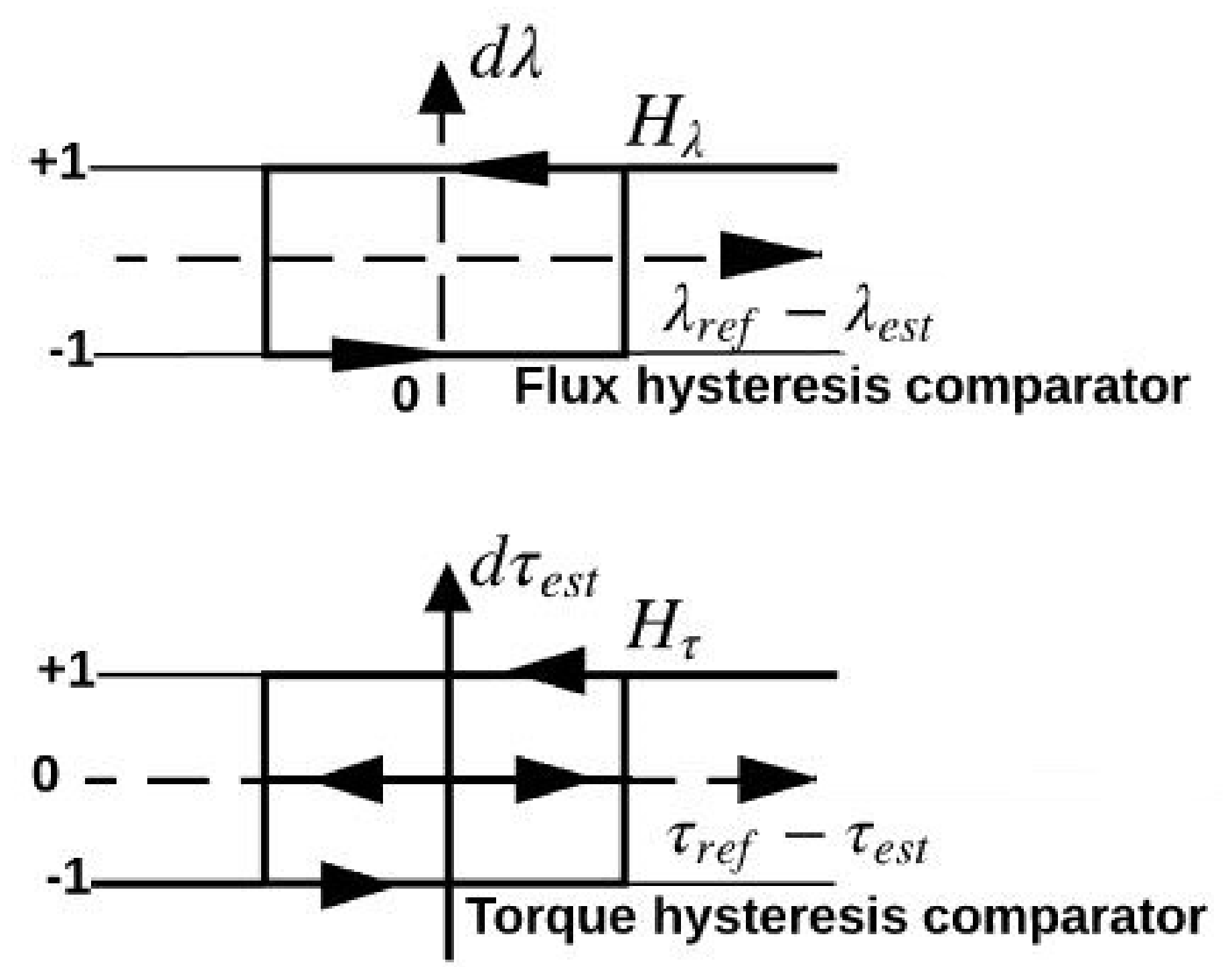
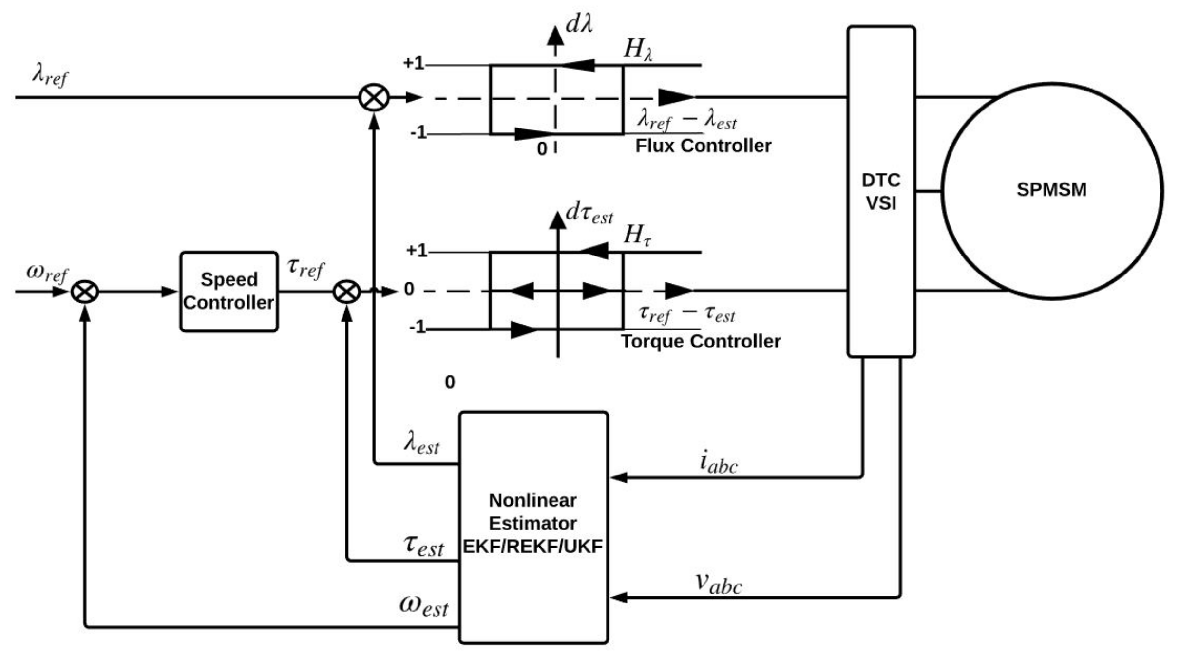
3. Direct Torque Control

Direct Torque control (DTC) was proposed by I. Takahashi for controlling induction motors in the mid 1980s [6,7]. The main feature of DTC is to apply appropriate voltage space vectors for voltage source inverter (VSI) from a predefined switching table. Voltage vectors with their position in space is shown in Figure 1. The six voltage space-vectors $(V_1-V_6)$ divides the space domain into six equal-area sectors. Either $V_0$ or $V_7$ can be used to represent a null vector at the origin. As DTC does not rely on pulse-width-modulation for generating the inverter voltage vectors, it requires less computational time with a reduced structure.

The overall scheme of the sensorless direct torque control with nonlinear Kalman filtering is shown in Figure 2. The desired stator flux ${\lambda }_{ref}$ and torque ${\tau }_{ref}$ are compared with the estimated stator flux ${\lambda }_{est}$ and torque ${\tau }_{est}$ in the hysteresis flux and torque controllers, respectively. The flux controller is a two-level hysteresis comparator, whereas the torque controller is a three-level hysteresis comparator. The flux and torque hysteresis comparators are illustrated in Figure 3.

The digitized output signal of the flux controller are defined based on

$$\begin{array}{ccc}\hfill d\lambda =1& for& {\lambda }_{est}<{\lambda }_{ref}-H_{\lambda }\hfill \end{array}$$

(25)

$$\begin{array}{ccc}\hfill d\lambda =0& for& {\lambda }_{est}>{\lambda }_{ref}+H_{\lambda },\hfill \end{array}$$

(26)

where $2H_{\lambda }$ is the flux tolerance band.

The digitized output signal of the torque controller are defined based on

$$\begin{array}{ccc}\hfill d{\tau }_{est}=1& for& {\tau }_{est}<H_{\tau }\hfill \end{array}$$

(27)

$$\begin{array}{ccc}\hfill d{\tau }_{est}=0& for& {\tau }_{est}=H_{\tau }\hfill \end{array}$$

(28)

$$\begin{array}{ccc}\hfill d{\tau }_{est}=-1& for& {\tau }_{est}>H_{\tau }\hfill \end{array}$$

(29)

where $2H_{\tau }$ is the torque tolerance band.

The stator flux sector index N is obtained from the computed angular position

$$\begin{array}{c}\hfill {\gamma }_s=ta{n}^{-1}\frac{{\lambda }_{\beta }}{{\lambda }_{\alpha }}\end{array}$$

(30)

Together with digitized variables $d\lambda$ and $d{\tau }_{est}$, a digital address for accessing an EPROM or EEPROM can be created. Hence, the appropriate voltage space-vector can be selected, which is governed by the switching rules in

Table 1. Direct Torque Control Switching Table.

$\mathit{d}\mathit{\lambda }$	$\mathit{d}{\mathit{\tau }}_{\mathit{est}}$	Number of Sectors (N)
		1	2	3	4	5	6
$d\lambda =1$	$d{\tau }_{est}=1$	$V_2$	$V_3$	$V_4$	$V_5$	$V_6$	$V_1$
	$d{\tau }_{est}=0$	$V_7$	$V_0$	$V_7$	$V_0$	$V_7$	$V_0$
	$d{\tau }_{est}=-1$	$V_6$	$V_1$	$V_2$	$V_3$	$V_4$	$V_5$
$d\lambda =0$	$d{\tau }_{est}=1$	$V_3$	$V_4$	$V_5$	$V_6$	$V_1$	$V_2$
	$d{\tau }_{est}=0$	$V_0$	$V_7$	$V_0$	$V_7$	$V_0$	$V_7$
	$d{\tau }_{est}=-1$	$V_5$	$V_6$	$V_1$	$V_2$	$V_3$	$V_4$

. Hence, the voltage source inverter can produce the desired three-phase voltages for controlling rotation.

4. Nonlinear Estimation

First, we revisit the traditional extended Kalman filter [28,29]. Over the past 40 years, EKF has been the most widely used nonlinear estimation technique for various industrial applications [30,31,32]. In order to provide a more reliable nonlinear estimation against external disturbances, noise, bad data and measurement failures, we propose the unscented Kalman filter (UKF) and the resilient extended Kalman filter (REKF)-based sensorless DTC technique for permanent magnet synchronous motors.

4.1. Extended Kalman Filter

Consider the discrete-time nonlinear system dynamics and measurement equation given as follows:

$$\begin{array}{c}\hfill x_{k+1}=f(x_k,u_k,v_k)\\ \hfill y_k=h(x_k,u_k,w_k)\end{array}$$

(31)

The extended Kalman filter estimation consists two steps: time update and measurement update.

First, define the following Jacobian matrices:

$$\begin{array}{c}\hfill A_k=\frac{\partial f}{\partial x}{{|}_{x={\widehat{x}}_k},F_k=\frac{\partial f}{\partial v}|}_{x={\widehat{x}}_k}\\ \hfill C_k=\frac{\partial h}{\partial x}{{|}_{x={\widehat{x}}_k},G_k=\frac{\partial h}{\partial w}|}_{x={\widehat{x}}_k}\end{array}$$

(32)

For time update, we compute the priori covariance and priori state estimate

$$\begin{array}{cc}\hfill P_k^{-}& =A_{k-1}{P}_{k-1}^{+}{A}_{k-1}^T+F_{k-1}{V}_{k-1}{F}_{k-1}^T\hfill \end{array}$$

(33)

$$\begin{array}{cc}\hfill {\widehat{x}}_k^{-}& =f_{k-1}({\widehat{x}}_{k-1}^{+},u_{k-1},0)\hfill \end{array}$$

(34)

where $V_k$ is the covariance matrix of process noise $v_k$ at time step k. ${\widehat{x}}^{-}$ is the priori state estimate and $P_k^{-}$ is the priori covariance matrix.

The measurement update can be summarized as follows

$$\begin{array}{c}\hfill K_k=P_k^{-}{C}_k^T{(C_k{P}_k^{-}{C}_k^T+G_k{W}_k{G}_k^T)}^{-1}\end{array}$$

(35)

$$\begin{array}{c}\hfill {\widehat{x}}_k^{+}={\widehat{x}}_k^{-}+K_k[y_k-h_k({\widehat{x}}^{-},0)]\end{array}$$

(36)

$$\begin{array}{c}\hfill P_k^{+}=(I-K_k{C}_k)P_k^{-}\end{array}$$

(37)

where ${\widehat{x}}_k^{+}$ is the posteriori state estimate; $P_k^{+}$ is the posteriori covariance matrix.

4.2. Resilient Extended Kalman Filter

Consider the discrete-time nonlinear stochastic system model and measurement equations as follows [33]:

$$\begin{array}{c}{x}_{k+1}=f\left(x_k\right)+v_k\\ y_k=\left(\begin{array}{c}{y}_k^1\\ y_k^2\\ ⋮\\ y_k^p\end{array}\right)=\left(\begin{array}{c}{\gamma }_k^1{h}^1\left(x_k\right)+w_k^1\\ {\gamma }_k^2{h}^2\left(x_k\right)+w_k^2\\ ⋮\\ {\gamma }_k^p{h}^p\left(x_k\right)+w_k^p\end{array}\right),\end{array}$$

(38)

where

• $x_k\in {\mathcal{R}}^n$ state vector
• $v_k\in {\mathcal{R}}^n$ system noise
• $y_k\in {\mathcal{R}}^n$ measurement vector
• $w_k^i\in \mathcal{R}$   measurement noise in each phasor
         measurement unit and $w_k={[w_k^1,w_k^2,\dots ,w_k^p]}^T$
• $f,h$     differentiable non-linear vector functions

The mean of initial state $x_o$ is $E\left[x_o\right]={\overline{x}}_o$ and covariance of initial state $x_0$ is $X_o=E[(x_o-{\overline{x}}_o){(x_o-{\overline{x}}_o)}^T]$. The process and measurement noises, $v_k$ and $w_k$, are white, zero mean, uncorrelated with each other and with $x_o$, and have covariance $V_k$ and $W_k$, respectively.

$$\begin{array}{c}\hfill v_k\sim (0,V_k),w_k\sim (0,W_k),\\ \hfill E[v_k{v}_j^T]=V_k{\delta }_{k-j},E[w_k{w}_j^T]=W_k{\delta }_{k-j},\\ \hfill E[v_k{w}_j^T]=0,E[v_k{x}_o^T]=0,E[w_k{x}_o^T]=0\end{array}$$

(39)

The scalar binary Bernoulli distributed random variables ${\gamma }_k^i$ are with mean ${\pi }_i$ and variance ${\pi }_i(1-{\pi }_i)$ whose possible outcomes 0,1 are defined as $Prob({\gamma }_k^i=1)={\pi }_i$ and $Prob({\gamma }_k^i=0)=1-{\pi }_i$. The formulation involves hard measurement failures, where the sensor either works properly or fails to provide reliable estimation.

By denoting

$$\begin{array}{c}\hfill {\Gamma }_k=diag[{\gamma }_k^1,{\gamma }_k^2,\dots ,{\gamma }_k^p]\end{array}$$

(40)

$$\begin{array}{c}\hfill h\left(x_k\right)=diag[h^1\left(x_k\right),h^2\left(x_k\right),\dots ,h^p\left(x_k\right)]\end{array}$$

(41)

the measurement equation can be written as

$$\begin{array}{c}\hfill y_k={\Gamma }_{k}h\left(x_k\right)+w_k\end{array}$$

(42)

Our goal is to estimate the state vector $x_k$ based on our knowledge of system dynamics and the availability of the noisy measurement $y_k$ under the effect of sensor failures. The following discrete time nonlinear Luenberger observer is considered in this work.

$$\begin{array}{c}\hfill {\widehat{x}}_{k+1}=f\left({\widehat{x}}_k\right)+(K_k+{\Delta }_k)(y_k-{\overline{\Gamma }}_{k}h\left({\widehat{x}}_k\right))\end{array}$$

(43)

Although the filter gain should be $K_k$, due to computational or tuning uncertainties, it is erroneously implemented as $K_k+{\Delta }_k$. The term ${\overline{\Gamma }}_k$ is defined as

$$\begin{array}{c}\hfill {\overline{\Gamma }}_k=E\left[{\Gamma }_k\right]=diag[{\pi }_1,{\pi }_2,\dots ,{\pi }_p]\end{array}$$

(44)

$K_k$ is the feedback gain with additive uncertainty ${\Delta }_k$. The uncertainty ${\Delta }_k$, is assumed to have zero mean, bounded second moment and be uncorrelated with initial state, process and measurement noises, i.e.,

$$\begin{array}{c}\hfill E[{\Delta }_k{\Delta }_k^T]\le \delta I,E[{\Delta }_k^T{x}_o]=0,E[{\Delta }_k^T{v}_k]=0,E[{\Delta }_k{w}_k]=0\end{array}$$

(45)

The resilient extended Kalman filter is defined as follows:

• Initialization

  $$\begin{array}{c}\hfill {\widehat{x}}_o=E[x_o]\\ \hfill P_o=E[(x_o-{\widehat{x}}_o){(x_o-{\widehat{x}}_o)}^T]\end{array}$$

  (46)
• Computation of Jacobian matrices

  $$\begin{array}{c}\hfill A_k=\frac{\partial f}{\partial x}{{|}_{x={\widehat{x}}_k},C_k=\frac{\partial h}{\partial x}|}_{x={\widehat{x}}_k}\end{array}$$

  (47)
• For time steps $k=1,2,3,\dots$, the estimator propagates by calculating the feedback gain

  $$\begin{array}{cc}\hfill K_k^o=& (A_k{P}_k{C}_k^T{\overline{\Gamma }}_k^T)[{\overline{\Gamma }}_k{C}_k{P}_k{C}_k^T{\overline{\Gamma }}_k^T+\hfill \\ & \mathrm{{\rm Y}}\otimes (h({\widehat{x}}_k)h^T({\widehat{x}}_k)+C_k{P}_k{C}_k^T)+W_k{]}^{-1}\hfill \end{array}$$

  (48)

  from an upper bound on the local estimation error covariance

  $$\begin{array}{c}{P}_{k+1}=A_k{P}_k{A}_k^T+V_k+{\lambda }_{max}\{{\overline{\Gamma }}_k{C}_k{P}_k{C}_k^T{\overline{\Gamma }}_k^T+W_k+\hfill \\ \mathrm{{\rm Y}}\otimes (h({\widehat{x}}_k)h^T({\widehat{x}}_k)+C_k{P}_k{C}_k^T)\}\delta I\hfill \\ -(A_k{P}_k{C}_k^T{\overline{\Gamma }}_k^T)[{\overline{\Gamma }}_k{C}_k{P}_k{C}_k^T{\overline{\Gamma }}_k^T+\hfill \\ \mathrm{{\rm Y}}\otimes (h({\widehat{x}}_k)h^T({\widehat{x}}_k)+C_k{P}_k{C}_k^T)+W_k{]}^{-1}({\overline{\Gamma }}_k{C}_k{P}_k{A}_k^T)\hfill \end{array}$$

  (49)

  to be used in updating the state estimate as

  $$\begin{array}{c}\hfill {\widehat{x}}_{k+1}=f\left({\widehat{x}}_k\right)+(K_k^o+{\Delta }_k)(y_k-{\overline{\Gamma }}_{k}h\left({\widehat{x}}_k\right))\end{array}$$

  (50)

  where

  $$\begin{array}{c}\hfill \mathrm{{\rm Y}}=diag[{\pi }_1(1-{\pi }_1),{\pi }_2(1-{\pi }_2),\dots ,{\pi }_p(1-{\pi }_p)]\\ \hfill =\left(\begin{array}{cccc}{\pi }_1(1-{\pi }_1)& 0& \cdots & 0\\ 0& \ddots & \ddots & ⋮\\ ⋮& \ddots & \ddots & 0\\ 0& \cdots & 0& {\pi }_p(1-{\pi }_p)\end{array}\right)\end{array}$$

  (51)

4.3. Unscented Kalman Filter

Consider the following system and measurement equations [34,35,36,37,38].

$$\begin{array}{c}\hfill x_{k+1}=f(x_k,u_k)+v_k\\ \hfill y_k=h\left(x_k\right)+w_k,\end{array}$$

(52)

where

• $f(x_k,u_k)$ process model
• $x_k$     state vectors
• $u_k$     input state vectors
• $h\left(x_k\right)$    output model
• $y_k$     output state vectors
• $v_k$     process WGN
• $w_k$    measurement WGN

The initial state $x_o$ has a mean ${\mu }_o=E\left[x_o\right]={\overline{x}}_o$ and a covariance $P_o=E[(x_o-{\mu }_o){(x_o-{\mu }_o)}^T]$. The process and measurement noise are white Gaussian noise (WGN), which can be expressed as $v_k\sim (0,V_k)$, $w_k\sim (0,W_k)$. The initial state variables obey normal distribution with ${\overline{x}}_o$ and $P_o$. The size of the sigma points is $x_k=2n+1$, from which the UKF can be implemented using the following steps:

• Initialization

  $$\begin{array}{c}\hfill {\widehat{x}}_o=E[x_o]\\ \hfill P_o=E[(x_o-{\overline{x}}_o){(x_o-{\overline{x}}_o)}^T]\end{array}$$

  (53)
• Define sigma points ${\chi }_k^{\left(s\right)}$ and weights ${\varpi }^s$ for $s=1,\cdots ,2n$ as follows:

  $$\begin{array}{c}\hfill {\chi }_k^{\left(0\right)}={\widehat{x}}_k\end{array}$$

  (54)

  $$\begin{array}{cc}\hfill {\chi }_k^{\left(s\right)}={\widehat{x}}_k+{\tilde{x}}_k^{\left(s\right)}& s=1,\cdots ,2n\end{array}$$

  (55)

  $$\begin{array}{cc}\hfill {\tilde{x}}_k^{\left(s\right)}={{\left(\sqrt{n{P}_k}\right)}_s}^T& s=1,\cdots ,n\end{array}$$

  (56)

  $$\begin{array}{cc}\hfill {\tilde{x}}_k^{(n+s)}=-{{\left(\sqrt{n{P}_k}\right)}_s}^T& s=1,\cdots ,n\end{array}$$

  (57)
  The weighing coefficients are determined by

  $$\begin{array}{cc}\hfill {\varpi }^s={\displaystyle \frac{1-{\varpi }^o}{2n}}& s=1,\cdots ,2n\end{array}$$

  (58)

  where the weight must agree

  $$\sum _{s=0}^{2n}{\varpi }^s=1.$$

  and ${\left(\sqrt{n{P}_k}\right)}_s$ is $s^{th}$ row or column of the matrix square root of $n{P}_k$.
• Process Update
  The priori mean and covariance of the estimated value ${\widehat{x}}_{k+1}^{-}$ can be obtained using the transformed sigma points as follows:

  $$\begin{array}{c}\hfill {\widehat{x}}_{k+1}=\sum _{s=0}^{2n}{\varpi }_s·f({\chi }_k^{(s)},u_k)\end{array}$$

  (59)

  $$\begin{array}{c}\hfill P_{k+1}^{-}=\sum _{s=0}^{2n}{\varpi }_s·(f({\chi }_k^{(s)},u_k)-{\widehat{x}}_{k+1}^{-}){(f({\chi }_k^{(s)},u_k)-{\widehat{x}}_{k+1}^{-})}^T+V_k\end{array}$$

  (60)
• Output Covariance Update
  The predicted measurement is

  $$\begin{array}{c}\hfill {\widehat{y}}_{k+1}=\sum _{s=0}^{2n}{\varpi }_s·h({\chi }_k^{(s)})\end{array}$$

  (61)

  $$\begin{array}{c}\hfill P_y=\sum _{s=0}^{2n}{\varpi }_s·(h({\chi }_k^{(s)})-{\widehat{y}}_{k+1}){(h({\chi }_k^{(s)})-{\widehat{y}}_{k+1})}^T+W_{k+1}\end{array}$$

  (62)
• Cross-correlation Update
  The cross-correlation $P_{xy}$ is determined by

  $$\begin{array}{c}\hfill P_{xy}=\sum _{s=0}^{2n}{\varpi }_s·(f({\chi }_k^{(s)})-{\widehat{x}}_{k+1}){(h({\chi }_k^{(s)})-{\widehat{y}}_{k+1})}^T\end{array}$$

  (63)
• Measurement Update
  The final measurement update can be performed using normal Kalman filter equations as: The Kalman gain $K_k$ can be written as follows:

  $$\begin{array}{c}\hfill K_{k+1}=P_{xy}P{{}_y}^{-1}\end{array}$$

  (64)
  The posteriori covariance matrix $P_{k+1}$ and the estimated state variable ${\widehat{x}}_{k+1}$ can be expressed as follows:

  $$\begin{array}{c}\hfill {\widehat{x}}_{k+1}={\widehat{x}}_{k+1}^{-}+K_{k+1}(y_{k+1}-{\widehat{y}}_{k+1})\end{array}$$

  (65)

  $$\begin{array}{c}\hfill P_{k+1}=P_{k+1}^{-}-K_{k+1}{P}_y{K}_{k+1}^T\end{array}$$

  (66)

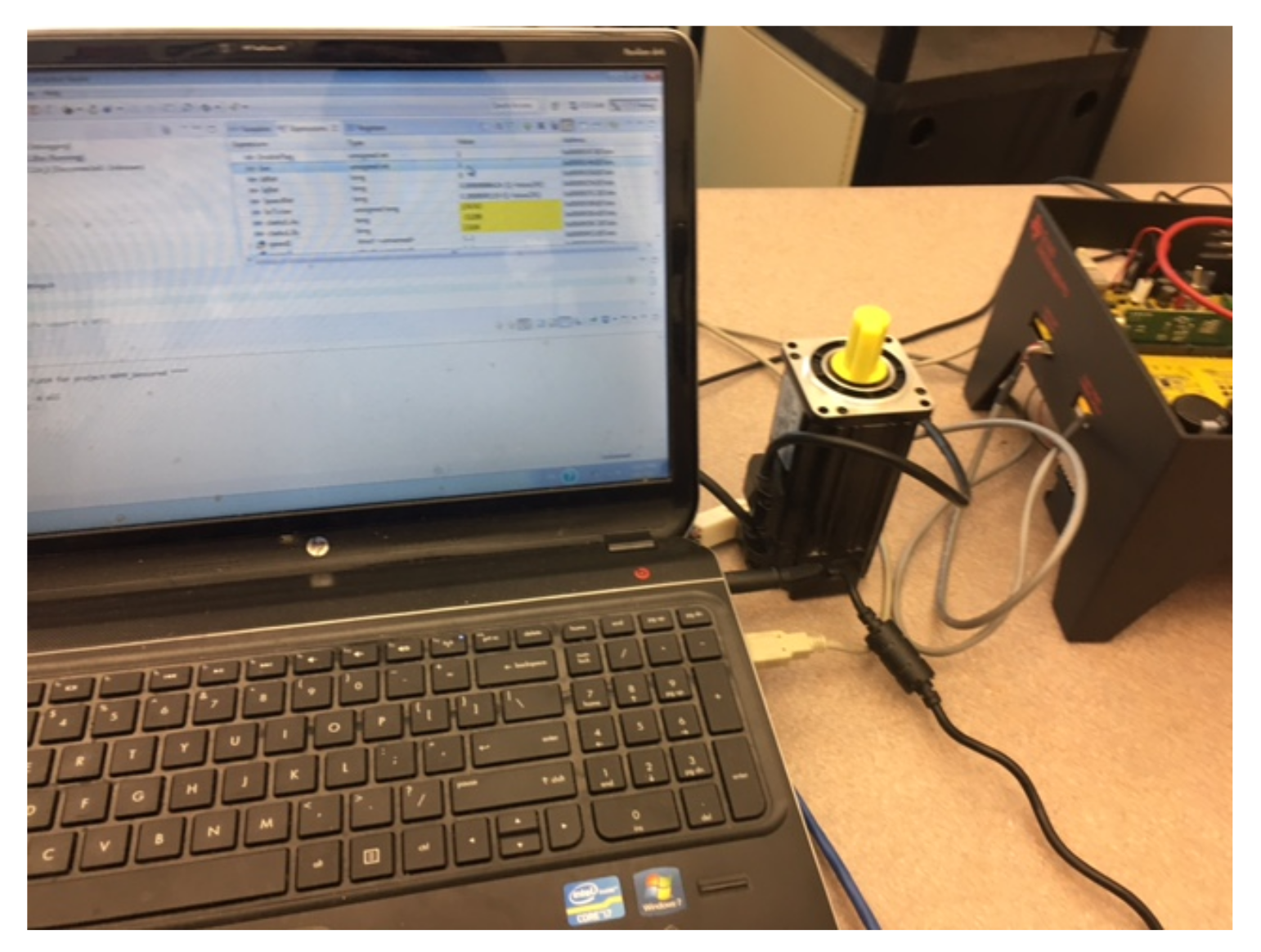
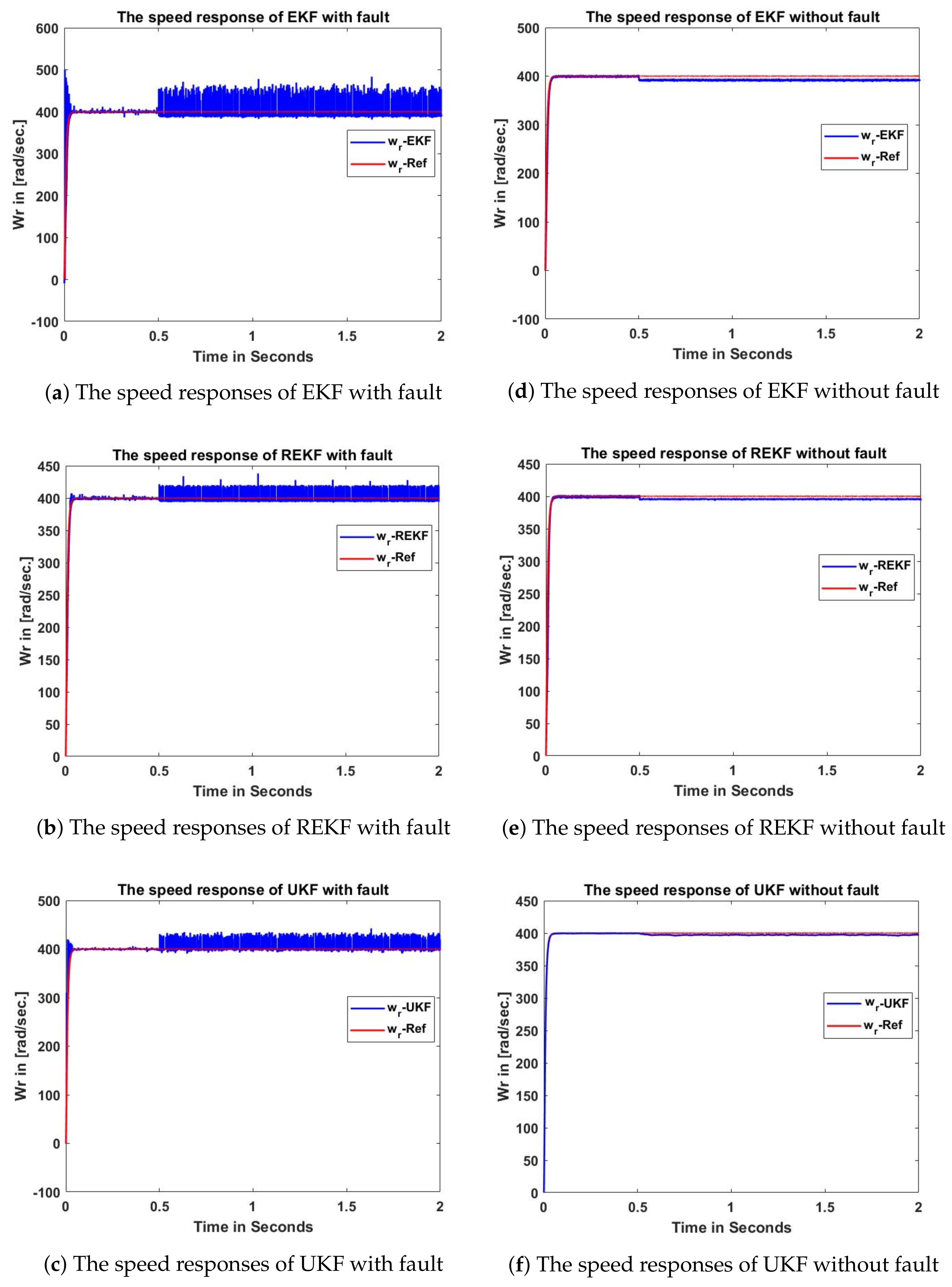
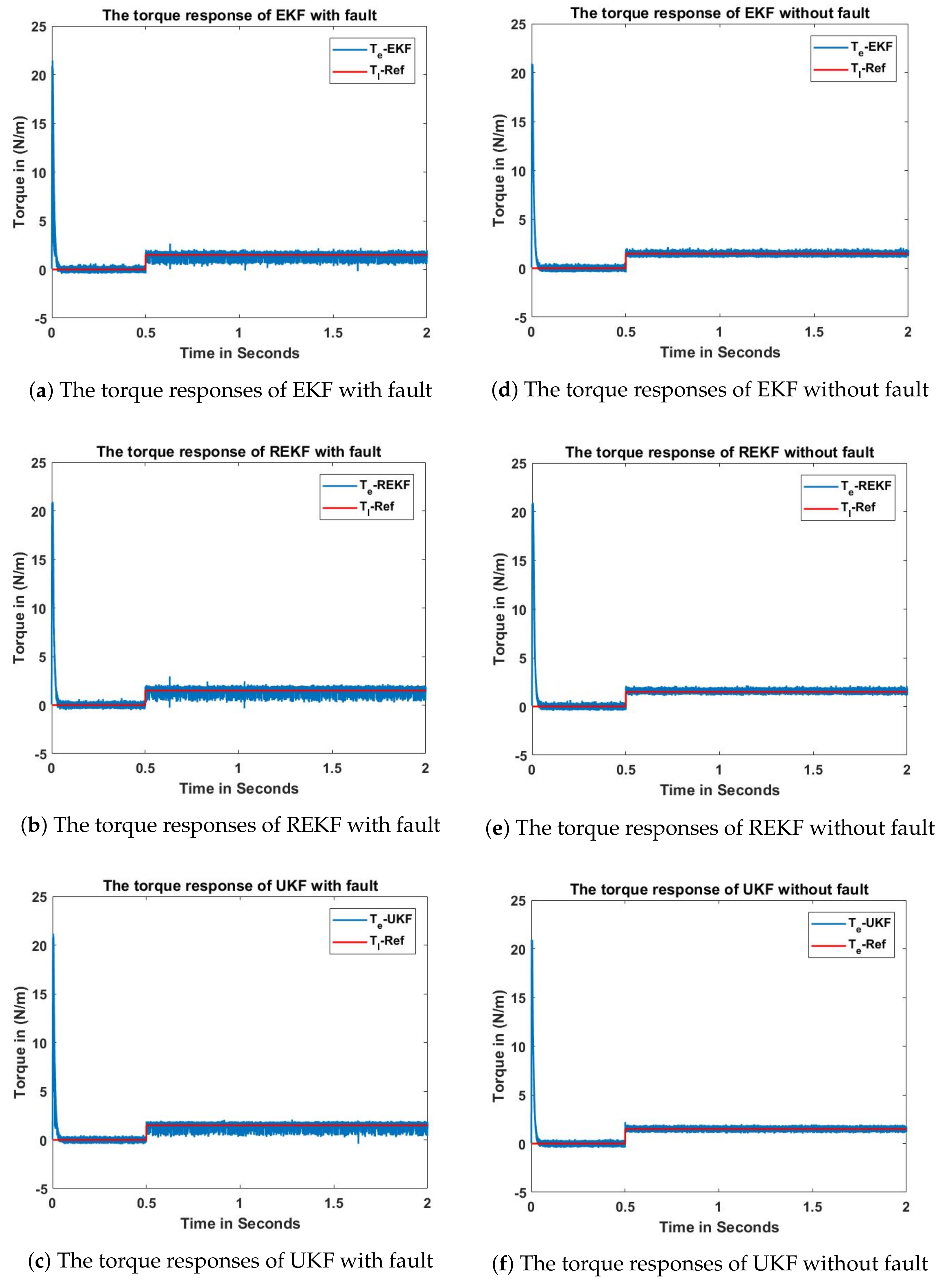
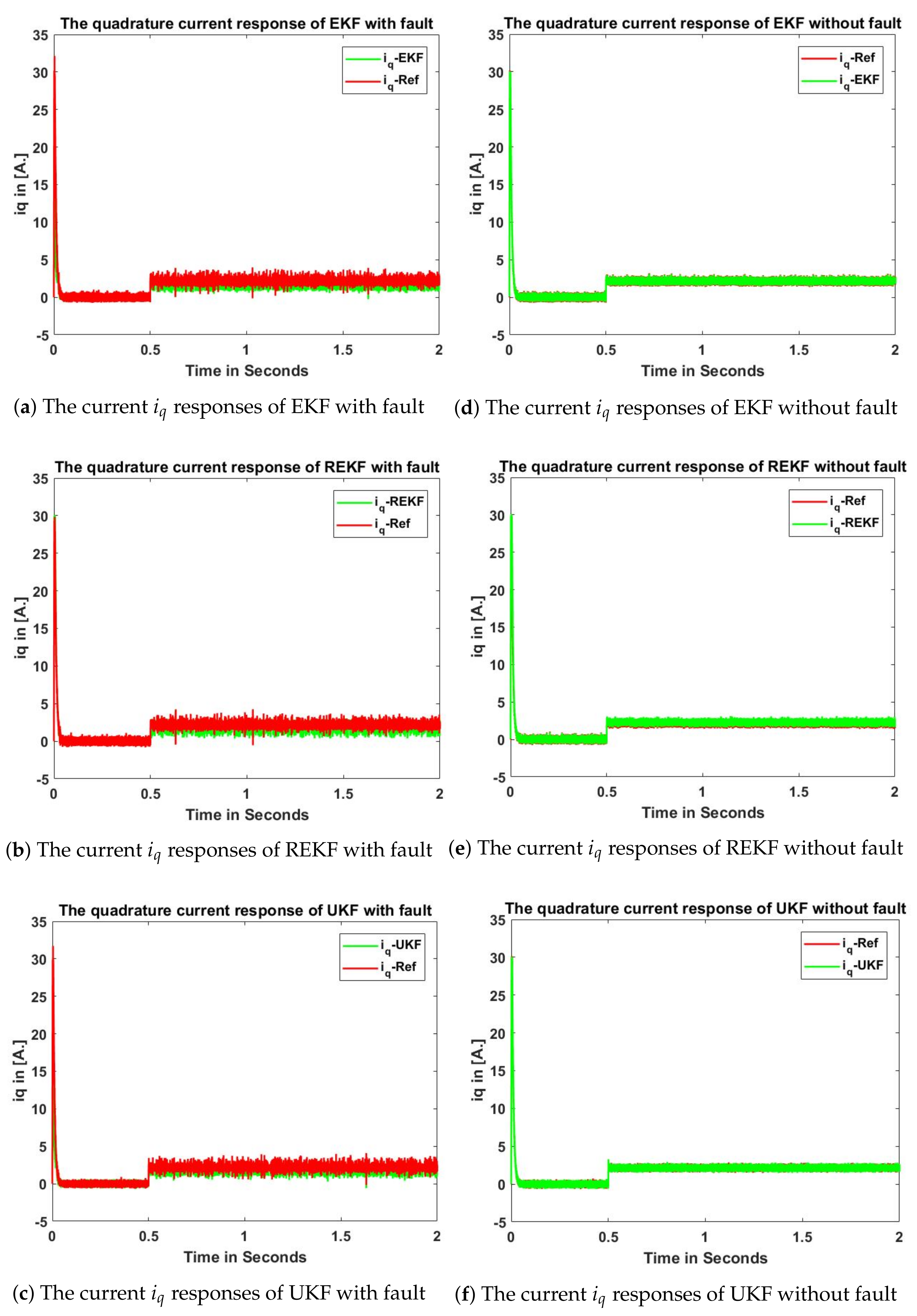
5. Computer Simulation Studies and Hardware Implementations

Computer simulation studies and Texas Instrument TMS320F28335 DSP processor implementations have been developed to show the efficiency of proposed sensorless direct torque control approach. The testing SPMSM parameters are summarized in

Table 2. The parameters of SPMSM.

Rated Power	400 W
Rated Torque	180 oz.in
Rated Voltage	220 V
Rated Current	2.7 A
Stator resistance, $R_s$	$4.7\mathsf{\Omega }$
Stator inductance, $L_s$	$13.3$ mH
Rotor magnetic flux, ${\lambda }_m$	$0.0785$ Wb
Number of rotor poles, P	8
Moment of inertia, J	$0.00439oz.in.s^2$

. The hardware implementation is shown in Figure 4.

The final reference speed of SPMSM motor is set to be 400 mechanical rad/s. An external load of 1.5 Nm is applied at 0.5 s. Figure 5, Figure 6, Figure 7 and Figure 8 show rotor speed, developed torque, stator flux, quadrature-axis stator current estimation comparisons, respectively. Figures in the first, second and third row show EKF, REKF and UKF estimation results, respectively. The first column figures are nonlinear estimation results under sensing failure condition. The second column figures are nonlinear estimation results without sensing failures. Note that EKF, UKF and REKF all converge to the real-state values. However, since the EKF uses first-order linearization to update the covariance of the state, it shows more estimation error compared with REKF and UKF.

Without measurement failures, the estimation error comparisons of EKF, UKF and REKF are summarized in

Table 3. The torque estimation error comparison of EKF, REKF, and UKF without sensor failure.

Time Period (s)	EKF Estimation Error (N/m)	REKF Estimation Error (N/m)	UKF Estimation Error (N/m)
0 s–0.5 s	0.6089	0.6692	0.6675
0.5 s–1.0 s	0.2188	0.1987	0.1348
1.0 s–1.5 s	0.2180	0.1951	0.1653
1.5 s–2.0 s	0.2197	0.1938	0.1067

,

Table 4. The $i_q$ estimation error comparison of EKF, REKF, and UKF without sensor failure.

Time Period (s)	EKF Estimation Error (A)	REKF Estimation Error (A)	UKF Estimation Error (A)
0 s–0.5 s	22.3889	22.4353	13.775
0.5 s–1.0 s	0.3985	0.3629	0.1491
1.0 s–1.5 s	0.3917	0.3718	0.2004
1.5 s–2.0 s	0.3971	0.3619	0.1842

and

Table 5. The speed estimation error comparison of EKF, REKF, and UKF without sensor failure.

Time Period (s)	EKF Estimation Error (rad/s)	REKF Estimation Error (rad/s)	UKF Estimation Error (rad/s)
0 s–0.5 s	10.7434	11.2876	1.7615
0.5 s–1.0 s	4.3493	3.0354	0.5825
1.0 s–1.5 s	4.3622	2.9833	0.7320
1.5 s–2.0 s	4.3790	3.0036	0.7345

. In comparison with EKF and REKF, UKF shows superior accuracy in torque, speed, and current estimation, under the condition that all sensors work properly. Under no sensing failure condition, UKF tracks the real state variables more closely with less ripples, since it relies on the unscented transformation to characterize the probability density function, without linearization involved. EKF truncates Taylor series of the mean at the first term, its prediction error of the mean value is in the second and higher order terms. EKF truncates at the first term of the covariance matrix, therefore, it is correct up to the second order with errors in fourth order term and above. UKF does not truncate any terms of the Taylor series, but uses sigma points through nonlinear transformation to decide the mean and covariance.

Under the sensing failure condition, computer simulations are conducted based on the assumption that each sensor has $5\%$ failure rate. Scalar binary random variables following Bernoulli distribution are generated for the measurements in order to produce random sensing failures. In another word, the sensor either works properly or fail to provide true measurements with a probability of $5\%$. In this case, the resilient extended Kalman filter provides more reliable state estimation with greater accuracy compared to EKF and UKF, since the resilient extended Kalman filter is designed to handle measurement failures. Hence, REKF is a more robust nonlinear estimation approach.

6. Conclusions

Direct torque control combines the benefits of direct flux and torque control into an adjustable speed drive, which does not require pulse-width-modulation or coordinate transforms. The paper presented a comparative study of sensorless direct torque control approaches of surface-mounted permanent magnet synchronous motors with the unscented Kalman filter (UKF), the resilient extended Kalman filter (REKF), and the extended Kalman filter (EKF). As demonstrated by simulation and implementation results, EKF, REKF, and UKF all track the state variables effectively. However, REKF is a preferred estimation method when sensors randomly fail to provide accurate measurements; whereas UKF is a superior method in state variables estimation when all sensors provide accurate measurements.

References

1. Xu, Z.; Rahman, M.F. Direct Torque and Flux Regulation of an IPM Synchronous Motor Drive Using Variable Structure Control Approach. IEEE Trans. Power Electron. 2007, 22, 2487–2498. [Google Scholar]
2. Cunha, J.P.V.S.; Costa, R.R.; Lizarralde, F.; Hsu, L. Peaking free variable structure control of uncertain linear systems based on a high-gain observer. Automatica 2009, 45, 1156–1164. [Google Scholar] [CrossRef]
3. Paicu, M.C.; Boldea, I.; Andreescu, G.D.; Blaabjerg, F. Very low speed performance of active flux based sensorless control: interior permanent magnet synchronous motor vector control versus direct torque and flux control. IET Electr. Power Appl. 2009, 3, 551–561. [Google Scholar] [CrossRef]
4. Boazzo, B.; Pellegrino, G. Model-Based Direct Flux Vector Control of Permanent-Magnet Synchronous Motor Drives. IEEE Trans. Ind. Appl. 2015, 51, 3126–3136. [Google Scholar] [CrossRef]
5. Drobnic, K.; Nemec, M.; Nedeljkovic, D.; Ambrozic, V. Predictive Direct Control Applied to AC Drives and Active Power Filter. IEEE Trans. Ind. Electron. 2009, 56, 1884–1893. [Google Scholar] [CrossRef]
6. Noguchi, T.; Takahashi, I. Quick torque response control of an induction motor based on a new concept. IEEJ Tech. Meeting Rotating Mach 1984, 1, 61–70. [Google Scholar]
7. Takahashi, I.; Noguchi, T. A new quick-response and high-efficiency control strategy of an induction motor. IEEE Trans. Ind. Appl. 1986, IA-22, 820–827. [Google Scholar] [CrossRef]
8. Rahman, M.F.; Zhong, L.; Haque, M.E.; Rahman, M.A. A direct torque-controlled interior permanent-magnet synchronous motor drive without a speed sensor. IEEE Trans. Energy Conver. 2003, 18, 17–22. [Google Scholar] [CrossRef]
9. Haque, M.E.; Rahman, M.F. Incorporating control trajectories with the direct torque control scheme of interior permanent magnet synchronous motor drive. IET Electr. Power Appl. 2009, 3, 93–101. [Google Scholar] [CrossRef]
10. Boldea, I.; Paicu, M.C.; Andreescu, G.D.; Blaabjerg, F. Active Flux DTFC-SVM Sensorless Control of IPMSM. IEEE Trans. Energy Conver. 2009, 24, 314–322. [Google Scholar] [CrossRef]
11. Faiz, J.; Mohseni-Zonoozi, S.H. A novel technique for estimation and control of stator flux of a salient-pole PMSM in DTC method based on MTPF. IEEE Trans. Ind. Electron. 2003, 50, 262–271. [Google Scholar] [CrossRef]
12. Buja, G.S.; Kazmierkowski, M.P. Direct torque control of PWM inverter-fed AC motors—A survey. IEEE Trans. Ind. Electron. 2004, 51, 744–757. [Google Scholar] [CrossRef]
13. Mohamed, Y.A.R.I. A Newly Designed Instantaneous-Torque Control of Direct-Drive PMSM Servo Actuator With Improved Torque Estimation and Control Characteristics. IEEE Trans. Ind. Electron. 2007, 54, 2864–2873. [Google Scholar] [CrossRef]
14. Mohamed, Y.A.R.I. Direct Instantaneous Torque Control in Direct Drive Permanent Magnet Synchronous Motors: a New Approach. IEEE Trans. Energy Conver. 2007, 22, 829–838. [Google Scholar] [CrossRef]
15. Boldea, I.; Agarlita, S.C. The active flux concept for motion-sensorless unified AC drives: A review. In Proceedings of the 2011 International Aegean Conference on Electrical Machines and Power Electronics and 2011 Electromotion Joint Conference (ACEMP), Istanbul, Turkey, 8–10 September 2011; pp. 1–16. [Google Scholar]
16. Vyncke, T.J.; Boel, R.K.; Melkebeek, J.A.A. A comparison of stator flux linkage estimators for a direct torque controlled PMSM drive. In Proceedings of the 35th Annual Conference of IEEE Industrial Electronics (IECON ’09), Porto, Portugal, 3–5 November 2009; pp. 971–978. [Google Scholar]
17. Inoue, Y.; Morimoto, S.; Sanada, M. Control Method Suitable for Direct-Torque-Control-Based Motor Drive System Satisfying Voltage and Current Limitations. IEEE Trans. Ind. Appl. 2012, 48, 970–976. [Google Scholar] [CrossRef]
18. Xu, Z.; Rahman, M.F. Comparison of a Sliding Observer and a Kalman Filter for Direct-Torque-Controlled IPM Synchronous Motor Drives. IEEE Trans. Ind. Electron. 2012, 59, 4179–4188. [Google Scholar] [CrossRef]
19. Mercorelli, P. A Two-Stage Sliding-Mode High-Gain Observer to Reduce Uncertainties and Disturbances Effects for Sensorless Control in Automotive Applications. IEEE Trans. Ind. Electron. 2015, 62, 5929–5940. [Google Scholar] [CrossRef]
20. Bernardes, T.; Montagner, V.F.; Gründling, H.A.; Pinheiro, H. Discrete-Time Sliding Mode Observer for Sensorless Vector Control of Permanent Magnet Synchronous Machine. IEEE Trans. Ind. Electron. 2014, 61, 1679–1691. [Google Scholar] [CrossRef]
21. Xu, Z.; Rahman, M.F. An extended Kalman filter observer for the direct torque controlled interior permanent magnet synchronous motor drive. In Proceedings of the Fifth International Conference on Power Electronics and Drive Systems, Singapore, 17–20 November 2003; pp. 686–691. [Google Scholar]
22. Xu, Z.; Rahman, M.F. Sensorless sliding mode control of an interior permanent magnet synchronous motor based on extended Kalman filter. In Proceedings of the Fifth International Conference on Power Electronics and Drive Systems, Singapore, 17–20 November 2003; pp. 722–727. [Google Scholar]
23. Foo, G.; Sayeef, S.; Rahman, M.F. SVM direct torque controlled interior permanent magnet synchronous motor drive using an extended Kalman Filter. In Proceedings of the 4th IET Conference on Power Electronics, Machines and Drives, York, UK, 2–4 April 2008; pp. 712–716. [Google Scholar]
24. Vyncke, T.J.; Boel, R.K.; Melkebeek, J.A.A. On Extended Kalman Filters with augmented state vectors for the stator flux estimation in SPMSMs. In Proceedings of the 2010 Twenty-Fifth Annual IEEE Applied Power Electronics Conference and Exposition (APEC), Palm Springs, CA, USA, 21–25 February 2010; pp. 1711–1718. [Google Scholar]
25. Mercorelli, P. A Hysteresis Hybrid Extended Kalman Filter as an Observer for Sensorless Valve Control in Camless Internal Combustion Engines. IEEE Trans. Ind. Appl. 2012, 48, 1940–1949. [Google Scholar] [CrossRef]
26. Mercorelli, P. A Two-Stage Augmented Extended Kalman Filter as an Observer for Sensorless Valve Control in Camless Internal Combustion Engines. IEEE Trans. Ind. Electron. 2012, 59, 4236–4247. [Google Scholar] [CrossRef]
27. Vyncke, T.J.; Boel, R.K.; Melkebeek, J.A.A. On the stator flux linkage estimation of an PMSM with Extended Kalman Filters. In Proceedings of the 5th IET International Conference on Power Electronics, Machines and Drives (PEMD 2010), Brighton, UK, 19–21 April 2010; pp. 1–6. [Google Scholar]
28. Reif, K.; Gunther, S.; Yaz, E.; Unbehauen, R. Stochastic stability of the discrete-time extended Kalman filter. IEEE Trans. Autom. Control 1999, 44, 714–728. [Google Scholar] [CrossRef]
29. Reif, K.; Gunther, S.; Yaz, E.; Unbehauen, R. Stochastic stability of the continuous-time extended Kalman filter. IEE Proc. Control Theory Appl. 2000, 147, 45–52. [Google Scholar] [CrossRef]
30. Haus, B.; Aschemann, H.; Mercorelli, P. Tracking Control of a Piezo-Hydraulic Actuator Using Input-Output Linearization and a Cascaded Extended Kalman Filter Structure. J. Franklin Inst. 2017. [Google Scholar] [CrossRef]
31. Mercorelli, P. An adaptive and optimized switching observer for sensorless control of an electromagnetic valve actuator in camless internal combustion engines. Asian J. Control 2014, 16, 959–973. [Google Scholar]
32. Chen, L.; Mercorelli, P.; Liu, S. A Kalman estimator for detecting repetitive disturbances. In Proceedings of the 2005 American Control Conference, Portland, OR, USA, 8–10 June 2005; Volume 3, pp. 1631–1636. [Google Scholar]
33. Wang, X.; Yaz, E.E. Stochastically resilient extended Kalman filtering for discrete-time nonlinear systems with sensor failures. Int. J. Syst. Sci. 2014, 45. [Google Scholar] [CrossRef]
34. Wan, E.A.; Van Der Merwe, R. The unscented Kalman filter for nonlinear estimation. In Proceedings of the Adaptive Systems for Signal Processing, Communications, and Control Symposium 2000 (AS-SPCC), Lake Louise, AB, Canada, 4 October 2000; pp. 153–158. [Google Scholar]
35. Wan, E.A.; Van Der Merwe, R. The Unscented Kalman Filter, Kalman Filtering and Neural Networks; John Wiley & Sons, Inc.: Hoboken, NJ, USA, 2002. [Google Scholar]
36. Julier, S.; Uhlmann, J. A New extension of the Kalman filter to Nonlinear Systems. In Proceedings Volume 3068, Signal Processing, Sensor Fusion, and Target Recognition VI; International Symposium Aerospace/Defense Sensing, Simulation and Controls, SPIE: Orlando, FL, USA, 1997; pp. 182–193. [Google Scholar]
37. Julier, S.; Uhlmann, J.K.; Durrant-Whyte, H.F. A new approach for filtering nonlinear systems. In Proceedings of the 1995 American Control Conference, Seattle, WA, USA, 21–23 June 1995; Volume 3, pp. 1628–1632. [Google Scholar]
38. Simon, D. Optimal State Estimation: Kalman, H-Infinity, and Nonlinear Approaches, 1st ed.; Wiley & Sons, Inc.: Hoboken, NJ, USA, 2006. [Google Scholar]
Figure 1. Voltage space vectors.
Energies 11 00969 g001
Figure 2. The proposed block diagram of DTC with nonlinear estimators.
Energies 11 00969 g002
Figure 3. The flux and torque hysteresis comparators.
Energies 11 00969 g003
Figure 4. Hardware Implementation with TMS320F28335 DSP.
Energies 11 00969 g004
Figure 5. The speed comparison of DTC with EKF, REKF, and UKF.
Energies 11 00969 g005
Figure 6. The torque comparison of DTC with EKF, REKF, and UKF.
Energies 11 00969 g006
Figure 7. The stator flux trajectory comparison of DTC with EKF, REKF, and UKF.
Energies 11 00969 g007
Figure 8. The current i q comparison of DTC with EKF, REKF, and UKF.
Energies 11 00969 g008