Article

Symbolic Analysis of the Cycle-to-Cycle Variability of a Gasoline–Hydrogen Fueled Spark Engine Model

by
Israel Reyes-Ramírez
1,
Santiago D. Martínez-Boggio
2,
Pedro L. Curto-Risso
2,
Alejandro Medina
3,
Antonio Calvo Hernández
3,* and
Lev Guzmán-Vargas
1
1
Unidad Profesional Interdisciplinaria en Ingeniería y Tecnologías Avanzadas (UPIITA)—Instituto Politécnico Nacional, Mexico City 07340, Mexico
2
Instituto de Ingeniería Mecánica y Producción Industrial, Universidad de la República, Montevideo 11300, Uruguay
3
Departamento de Física Aplicada, Facultad de Ciencias, Universidad de Salamanca, Salamanca 37008, Spain
*
Author to whom correspondence should be addressed.
Energies 2018, 11(4), 968; https://doi.org/10.3390/en11040968
Submission received: 7 March 2018 / Revised: 13 April 2018 / Accepted: 15 April 2018 / Published: 18 April 2018

Abstract

:
An study of temporal organization of the cycle-to-cycle variability (CCV) in spark ignition engines fueled with gasoline–hydrogen blends is presented. First, long time series are generated by means of a quasi-dimensional model incorporating the key chemical and physical components, leading to variability in the time evolution of energetic functions. The alterations in the combustion process, for instance the composition of reactants, may lead to quantitative changes in the time evolution of the main engine variables. It has been observed that the presence of hydrogen in the fuel mixture leads to an increased laminar flame speed, with a corresponding decrease in CCV dispersion. Here, the effects of different hydrogen concentrations in the fuel are considered. First, it is observed that return maps of heat release sequences exhibit different patterns for different hydrogen concentrations and fuel–air ratios. Second, a symbolic analysis is used to characterize time series. The symbolic method is based on the probability of occurrence of consecutive states (a word) in a symbolic sequence histogram (SSH). Modified Shannon entropy is computed in order to determine the adequate word length. Results reveal the presence of non-random patterns in the sequences and soft transitions between states. Moreover, the general behavior of CCV simulations results and three types of synthetic noises: white, log-normal, and a noisy logistic map, are compared. This analysis reveals that the non-random features observed in heat release sequences are quite different from synthetic noises.

1. Introduction

Present-day automotive engines are considerably more complex than several years ago, due to the increasingly stringent emission regulations and the demand for fuel-efficient vehicles [1]. Diagnosis of combustion is necessary to check combustion quality and to design appropriate control algorithms [2]. In particular, the diagnosis and control of cycle-to-cycle variability (CCV) is a subject that has been deeply researched in recent times. One possible action to limit variability effects in gasoline-fueled spark-ignition engines is the addition of additives with a high laminar flame speed to the main fuel. Any effort associated to increasing the flame speed, in principle, will be positive in order to decrease variability fluctuations.
The use of hydrogen as an additive in gasoline–hydrogen blends improves combustion speed and reduces CCV amplitude because of hydrogen’s high laminar flame speed. On the contrary, it has disadvantages such as the energy consumption required for its production, storage difficulties, and the technical modifications needed for standard spark ignition engines. The main positive features and drawbacks of using hydrogen as engine fuel have been summarized by several authors [3,4,5].
Most studies on the effects of hydrogen addition on variability are experimental. D’Andrea et al. [6] calculated the coefficient of variation (COV) of the indicated mean of effective pressure (IMEP) and the mass fraction burned for 100 individual cycles. A decrease of CCV for lean operation (fuel–air equivalence ratio ϕ below 0.85) was found. In close to stoichiometric conditions, scarce differences in engine performance were seen. Ji and co-workers [7,8,9,10,11] calculated the COV of IMEP for 300 cycles for a 1.6 L four-stroke commercial engine when idle (around 790 rpm) with a hydrogen volume fraction in the total intake gas of 6.52 % . An appreciable decrease of the COV of IMEP when plotted in terms of the hydrogen energy fraction was observed. In subsequent work [8], for a similar engine and identical number of cycles, the COV of IMEP was obtained as a function of the excess air ratio, λ , between 1.0 and 1.7. The progressive addition of hydrogen to gasoline prevented a rapid increase of the COV of IMEP when using lean mixtures. The influence of spark timing was analyzed in [9], also for 300 consecutive cycles. Recently, the engine performance at wide open throttle condition was analyzed and the COV of IMEP measured [10,11].
Several zero- and multi-dimensional thermodynamic models have been developed for predicting engine performance parameters and emissions in gasoline–hydrogen fueled engines. A complete review was performed by Verhelst and Wallner [5]. Nevertheless, usually, these models do not deeply represent the effect of hydrogen addition on CCV. Also, different Computational Fluid Dynamics (CFD) schemes were proposed [5,12,13]. However, as occurs in experimental calculations, obtaining long time series and statistically significant results is not easy [2,14,15]. Usually, just a few hundred of cycles are computed, and thus, to analyze long time series and correlations of the evolution of variables such as IMEP, heat release, or power output, further work is necessary.
With respect to the analysis of the time series displaying cyclic variability (maximum pressure, IMEP, heat release, power output, etc.), several techniques have been used: stochastic modeling [15,16], concepts derived from information theory and statistical thermodynamics [17], return maps and recurrence plots [18,19], fractal and multifractal analysis [20,21,22], wavelets [20,23], symbolic analysis [24,25,26,27,28], etc. Many authors have reported that the use of symbolic analysis is useful as a diagnostic tool in order to predict future cycles that could be used in control algorithms. As emphasized by Chen et al. [27], symbol sequence statistics constitute a relatively simple and effective approach to minimize dynamic noises and analyze possible deterministic prior-cycle effects. The pattern structure repeated in consecutive cycles, if existing, can be applied to predict future cycle evolution and so help to enable control mechanisms.
A quasi-dimensional simulation scheme for spark ignition engines was developed by our research group in recent years. The model takes into account valve overlapping, heat transfer from the cylinder to the coolant, the effects of residual gases from previous cycles, specific turbulent flow models, and turbulent combustion in the chamber. It is especially suitable for the analysis of CCV because it is feasible to obtain long time series with a reduced computational cost. Variability is incorporated by introducing several random components of basic parameters of combustion such as the typical size of unburned eddies inside the flame front. It has been shown in several publications that the model is able to simulate average engine records as well as variability effects for engines fueled with pure gasoline [22,29,30], gasoline–ethanol blends [23], and gasoline–hydrogen blends [31]. Recently, time series for the power output were presented and analyzed by using standard statistical metrics [31]. It was found that the addition of hydrogen decreases the dispersion of the time series without a significant decrease in power output. Moreover, it was shown that for each fuel–air ratio concentration, there exists a particular optimum hydrogen concentration by volume at which the coefficient of variation is minimal.
In this work, long time series ( 10 4 cycles) of simulated heat release are analyzed in order to study the effect of different hydrogen blend concentrations (the notation % H 2 will be used throughout the work to refer to the percentage of hydrogen per volume in the total fuel volume) on the reduction of fluctuations of CCV for several relative fuel–air ratios, ϕ . To this end, symbolic analysis is used to survey and quantify possible structures in heat release sequences and their corresponding return maps [1,17,19,32,33,34]. The paper is organized as follows: in Section 2, the developed quasi-dimensional model is described, giving details of the combustion model and chemical reactions considered. Also, the main aspects of the concordance between model predictions and some experimental measurements with validation purposes are presented. In Section 3 the simulated time series are described, highlighting the objectives of the subsequent symbolic analysis. In Section 4 the theoretical framework of the symbolic analysis is provided, including the use of a modified Shannon entropy in order to find the best optimal pattern length characterizing the deterministic structure. Then, three well-known random processes as a framework to compare simulations are described. In Section 5, findings on the symbolic analysis are presented, with special emphasis on describing the changes in the dynamics for different combinations of values of ϕ and % H 2 . Finally, some general conclusions are presented.

2. Quasi-Dimensional Simulation Model

Over recent years a quasi-dimensional model for spark ignition engines capable of reproducing the observed phenomenology related with cycle-to-cycle fluctuations has been developed. The model has been described in detail in several publications [31,35,36], so here the main theoretical framework is briefly outlined. From the theoretical viewpoint the model starts from stating the first principle of thermodynamics for open systems as a set of coupled differential equations for temperature and pressure inside the combustion chamber. The considered control volume is determined by the cylinder inner wall. The working fluid is an adiabatic mixture of unburned (u) and burned (b) gases except during combustion, where a two-zone scheme is taken. All gases are assumed as ideal with temperature-dependent specific heats. The heat capacity ratio for the burned gases is calculated from the equilibrium composition at any time instant. Enthalpy changes are only associated to temperature changes except during combustion, where species redistribution according to chemical reactions is taken into account.
From energy and mass conservation laws, a system of differential equations for pressure and temperature inside the combustion chamber is developed (explicit equations can be found in [31]). These coupled equations are valid during all stages (including the overlapping period where intake and exhaust valves are simultaneously open), except for combustion. Particular models are required for all cycle processes. The mass flow rates through the valves are calculated by means of the standard equations for the isentropic flow of a compressible fluid through an orifice [37]. For friction components, the empirical correlation by Barnes–Moss is considered, including both linear and quadratic terms on engine speed [38]. The heat transfer between the gas inside the cylinder and the cylinder inner wall is modeled with Eichelberg’s correlation [39].
In the combustion time lapse two different control volumes are considered. They are separated by the flame front. The initial temperature of burned gases is taken as the adiabatic flame temperature at constant pressure. The pressure is considered as uniform during all this period [37,40]. In the next section the details of the combustion model are described.

2.1. Combustion Model

For the combustion process, the model developed by Keck and coworkers [41,42] is assumed. Combustion is considered as turbulent. In the course of flame propagation, the flame front is supposed approximately spherical but not all the mass inside is burned; there are vortices or eddies of unburned gases. They have a characteristic length, l t , related to the Taylor microscale or turbulence length scale [43]. The set of coupled differential equations that gives the time evolution of the total mass inside the flame front, m e (this is the total mass inside the flame front, unburned and burned gases), and the mass of burned gases, m b , is written as:
m ˙ b = F w A f ρ u S L + m e m b τ b
m ˙ e = F w A f ρ u u t 1 e t / τ b + S L
where t stands for the time from the beginning of combustion and A f for the area of the flame front is assumed as spherical. It is calculated from the volume of gases inside the flame front, V f [36,40]. This volume is given by V f = V ( m m e ) / ρ u where V is the total cylinder volume, ρ u is the density of unburned gases, and m is the total mass of the gases in the cylinder. The parameter F w represents the flame front wrinkling, associated to the addition of hydrogen [13]. This point will be detailed below. The first addend at the right of Equation (1) represents the laminar propagation of the flame front, and the second the combustion of the fresh mixture inside the flame front. The time parameter τ b = l t / S L , is the characteristic time required for the combustion of a vortex of typical length, l t , at the laminar flame speed, S L . From another viewpoint, τ b is the time the flame front needs to develop into a turbulent flame from the initial conditions: an initial spherical kernel evolving at laminar flame speed [44]. Equation (2) describes the total mass inside the flame front rate that evolves at a velocity, u t + S L , ( t > > τ b ), where u t is the characteristic speed of the mixture when crossing the flame front. It is associated to turbulence intensity [43]. During combustion these equations are coupled to the set of thermodynamic ones.
The correlation by Metghalchi and Keck [45,46] for the dependence of the laminar flame speed on temperature and pressure is assumed,
S L = S L , 0 T u T ref α p p ref β ( 1 2.1 y r 0.77 )
In this correlation, T u is the temperature of unburned gases in the chamber, p is the pressure, and y r is the mole fraction of residual gases from the previous cycle. T ref and p ref are reference values. For isooctane–hydrogen blends, the reference laminar speed, S L , 0 , and the exponents α and β were taken from the work of Ji et al. [13]. They considered mixtures up to 85 % hydrogen in volume in the incoming fresh air and broad intervals for fuel–air ratios, temperatures, pressures, and residual gases mass fractions.
Undoubtedly, flame surface wrinkling in spark ignition engines is associated to turbulence [47,48]. The combustion reaction rate and combustion duration determine the wrinkling degree. Due to the high thermal and mass diffusivities of hydrogen, its addition to a fuel could reduce flame thickness [13,49]. In consequence, hydrogen-enriched flames are even more sensitive to local turbulence and thus, experience further wrinkling.
In this paper, wrinkling effects are incorporated in the numerical value of the flame front area. In Equations (1) and (2), the flame front area is multiplied by a factor F w that fits the difference between a smooth spherical flame front and a wrinkled one. From the data obtained by Ji et al. [13] through CFD simulations in the same conditions considered here, a correlation between the concentration of hydrogen in the blend per unit volume and F w is fitted [31]: F w = 0.41737 y H 2 + 1 , where y H 2 is the ratio of hydrogen volume in the total fuel (isooctane and hydrogen) volume. This function is appropriate for blends of up to 80 % hydrogen per volume in the mixture. Details can be surveyed in [8,13]. The increase in flame wrinkling together with the increase of the laminar speed when hydrogen is added to the fuel provoke a boosting of flame front propagation, and so a reduction in combustion time span.

2.2. Chemical Reactions

The chemical reaction for combustion was solved assuming chemical equilibrium conditions, including dissociation. Isooctane (as fuel reference for gasoline), hydrogen, dry air, and previous cycle reaction products were considered as reactants. The method presented by Ferguson [50] to solve chemical equilibrium for ten species, including residual gases from the previous cycle, is applied. The equation for chemical equilibrium reads:
( 1 y r ) 1 + ε ϕ ε ϕ ( 1 y H 2 ) C 8 H 18 + y H 2 H 2 + 0.21 O 2 + 0.79 N 2 + + y r y 1 C O 2 + y 2 H 2 O + y 3 N 2 + y 4 O 2 + y 5 C O + y 6 H 2 + y 7 H + y 8 O + y 9 O H + y 10 N O ν 1 C O 2 + ν 2 H 2 O + ν 3 N 2 + ν 4 O 2 + ν 5 C O + ν 6 H 2 + ν 7 H + ν 8 O + ν 9 O H + ν 10 N O
The factor ε depends on the hydrogen concentration [31]. The factors, ν i , on the right-hand side are the ratios between the mole number of each species and the moles of reactants. These coefficients are obtained by stating a set of algebraic equations resulting from the conservation of the number of atoms of each species [50].
It is convenient to stress that complete oxidation was considered, i.e., burned gas consisting of CO2, H2O, N2, and O2 for lean combustion. While this assumption can be viewed as a source of errors in the simulations, several works show that the main influence on combustion modeling is through S L and T u , as pointed out by several authors [51,52]. Moreover, note that the stated chemical reaction does not explicitly consider a detailed composition of combustion products with respect to hydrogen. This is because the main focus of this work is placed on the energetics in terms of cycle-to-cycle heat release in the engine. Furthermore, the explicit estimation of NO x emissions would require non-equilibrium reaction models that are out of the scope of this work [31]. Therefore, the effect of the hypothesis of chemical equilibrium on the calculations hereafter shown in the work is negligible.

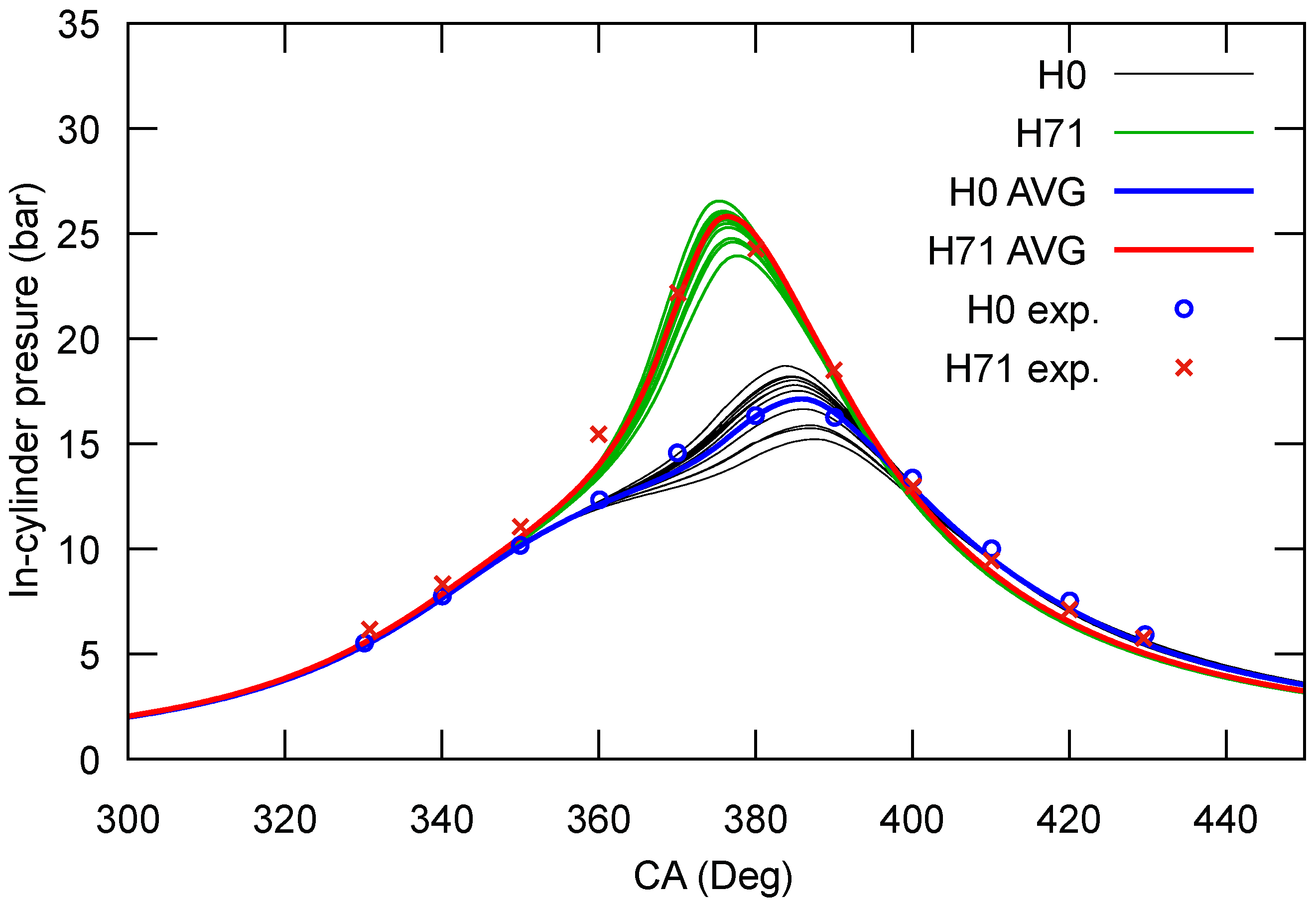
2.3. Simulation Validation and Heat Release Time Series Computation

Simulation validation was divided in two steps. First, before the incorporation of cyclic variability, model predictions with average experimental measures were compared. The engine parameters were elected to fit the experimental results by Ji et al. [8]. They are summarized in Table 1. The engine speed for simulations was taken as 1400 rpm and the spark advance 22°crank angle before top dead center (CA BTDC), the same values as in experiments. Validation relies on the comparison of curves for the simulated pressure inside the cylinder, as well as the burned gas mass fraction during combustion. If the evolution of pressure with the crank angle resembles experimental results, it could be concluded that predictions for indicated power are accurate. Similarly, if the simulated evolution of the burned gases mass fraction is similar to the experimental one, it could be confirmed that energy release rate is well reproduced. Thus, efficiencies will be alike. The figures comparing experiments and model predictions are not explicitly shown, but can be checked in [31]. The agreement is quite satisfactory. For the pressure the relative deviations are always below 5% and more than 90% of the computed points have a deviation under 2%. Deviations for the burned gases mass fraction are even smaller.
In a second step, cyclic variability is incorporated in the simulation scheme, and its predictions are compared with experimental results available in the literature. Hence, the next aim is to model cycle-to-cycle fluctuations within the computational scheme. It is widely considered that the main physical ingredients of variability in spark ignition engines are: turbulence during gas motion in the cylinder (including combustion), homogeneity of the mixture in near the spark plug, and the memory effects coming from the existence in the chamber of previous cycle residual gases [36,53,54]. Variability fluctuations are larger for lean mixtures and low engine speeds.
In the computational model, the laminar flame speed S L , connects the evolution of combustion in a given cycle with the mole fraction of residual gases from the previous one, y r (see Equation (3)), i.e., it links the combustion chemistry of one cycle with the preceding one. Furthermore, there are other parameters that determine the flame front expansion: the typical length of the unburned gas eddies inside the flame front, l t , the typical speed at which the mixture crosses the flame front, u t (linked to turbulence intensity), and the location of the ignition kernel [55]. Previous studies [30,36] showed that stochastic components of l t or u t need to be added in order to reproduce the experimental phenomenology of CCV. Actions contributing to increase the turbulence intensity in the cylinder favor the reduction of variability. Nevertheless, this usually causes a reduction in volumetric efficiency at high speeds. Thus, other mechanisms that could increase flame speed without affecting cycle performance at high speed are nowadays sought [6]. One possible option is to modify the fuel in the engine, with additives showing a high laminar flame speed. In this context, hydrogen, due to its high flame speed and diffusivity, is a choice to analyze.
A random component on l t at the beginning of combustion (in each cycle) is introduced in numerical computations. It evolves thereafter with the ratio of the densities of the burned and unburned gas mixture (see [36] for details). The empirical correlations developed by Beretta [42] are considered. They only depend on the mean inlet gas speed and on the maximum valve lift, not on the chemical composition of the mixture. The random component of l t is obtained by comparing the coefficient of variation (COV) of the IMEP (defined as the ratio between the standard deviation and the mean) as calculated in the model with the experimental data presented by Ji et al. [56] for pure gasoline, % H 2 = 0 . This procedure ensures to reproduce the experimental dispersion associated to cyclic variability. Figure 1 displays the comparison of simulation predictions for the COV of IMEP after 10 4 cycles with the experimental results of Ji et al. [56]. Three hydrogen concentrations are shown: H0 (pure isooctane), H71 (71% H2 by volume), and H85 (85% H2), and the fuel–air ratio is varied from 0.7 to stoichiometric conditions. The decrease of variability for increasing hydrogen concentration and increasing fuel–air ratio is evident from the figure. More details on the validation procedure can be found in [31].
It is interesting to show how variability is directly reflected in the evolution of pressure during combustion. This is analyzed in Figure 2 for two levels of hydrogen concentration and a fixed lean mixture fuel–air ratio, ϕ = 0.79 . In the plot several cycles are displayed as well as the average values of pressure and the experimental findings by Ji et al. [8]. Simulations correctly reproduce average curves and the increasing of maximum pressure with increasing concentration of hydrogen.
One of the main advantages of quasi-dimensional simulations in the analysis of cyclic variability is its capability to obtain long time series in a reduced computational time. Usually, experimental measures deal with a few hundred cycles. This makes difficult to obtain representative information about possible correlations in time series. Nevertheless, by means of quasi-dimensional simulations it is feasible to obtain time series on the order of several thousands of cycles, which allows for good precision in the estimation of statistical parameters as well as analysis of the time dynamics of any engine variable.

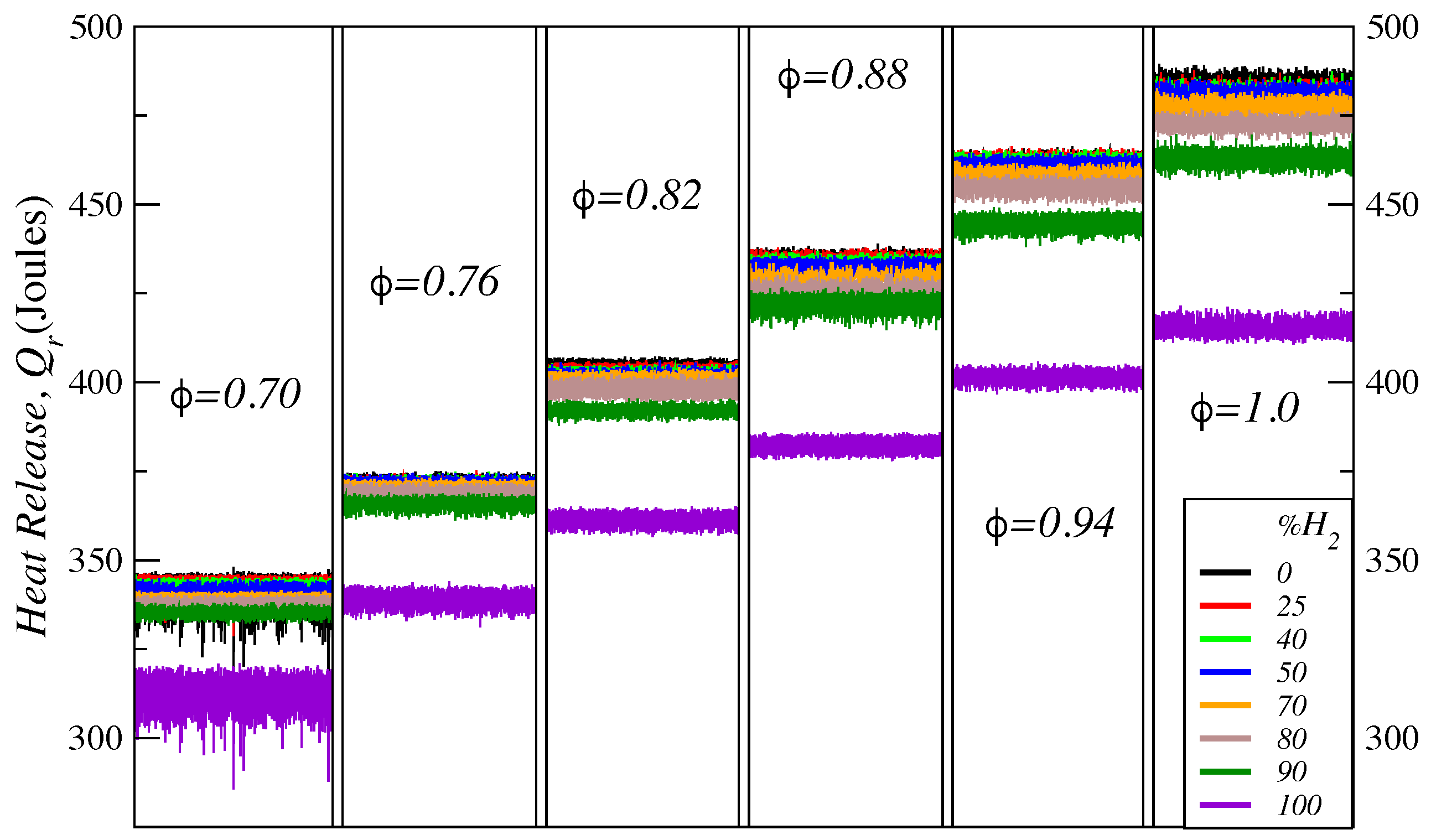
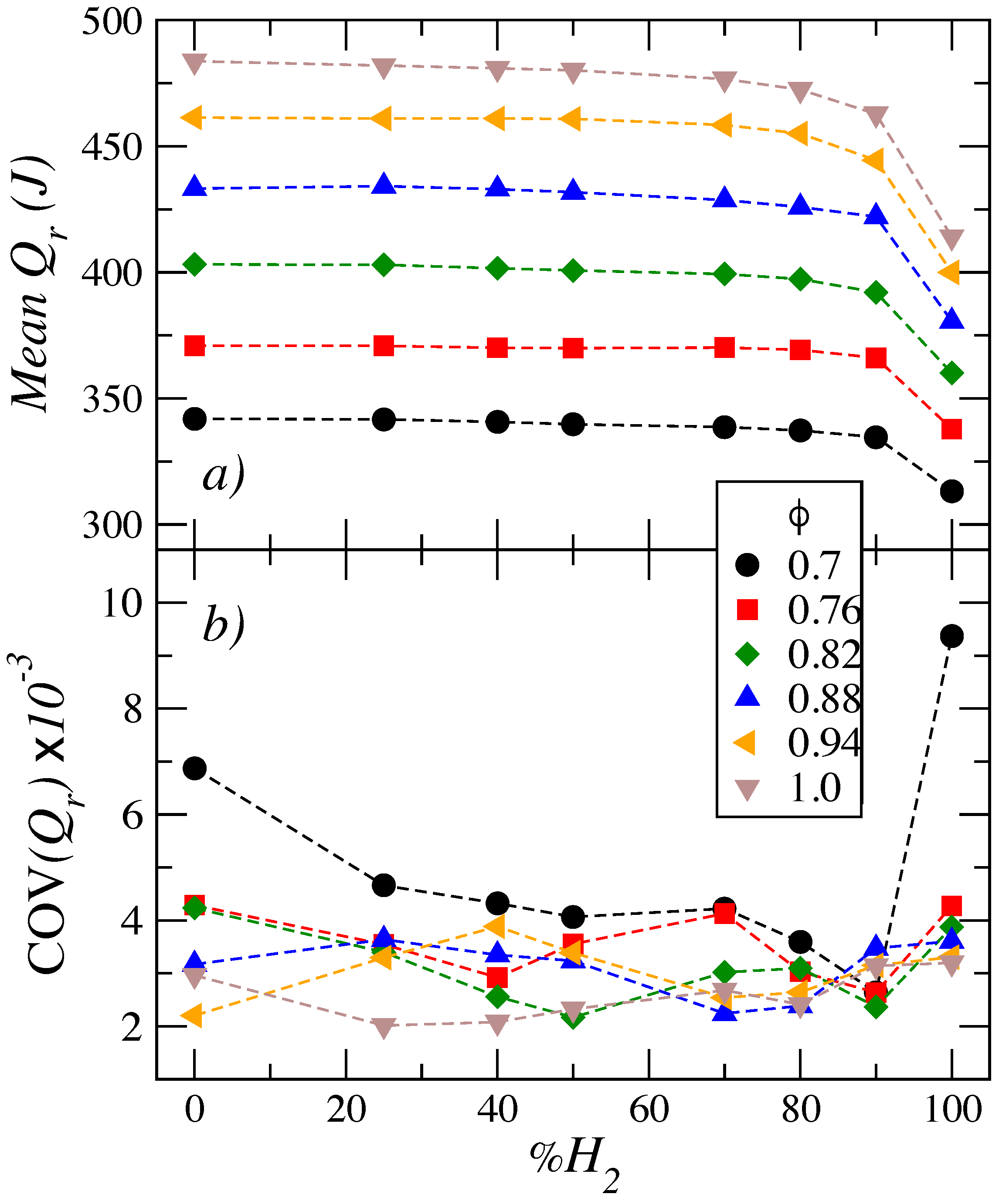
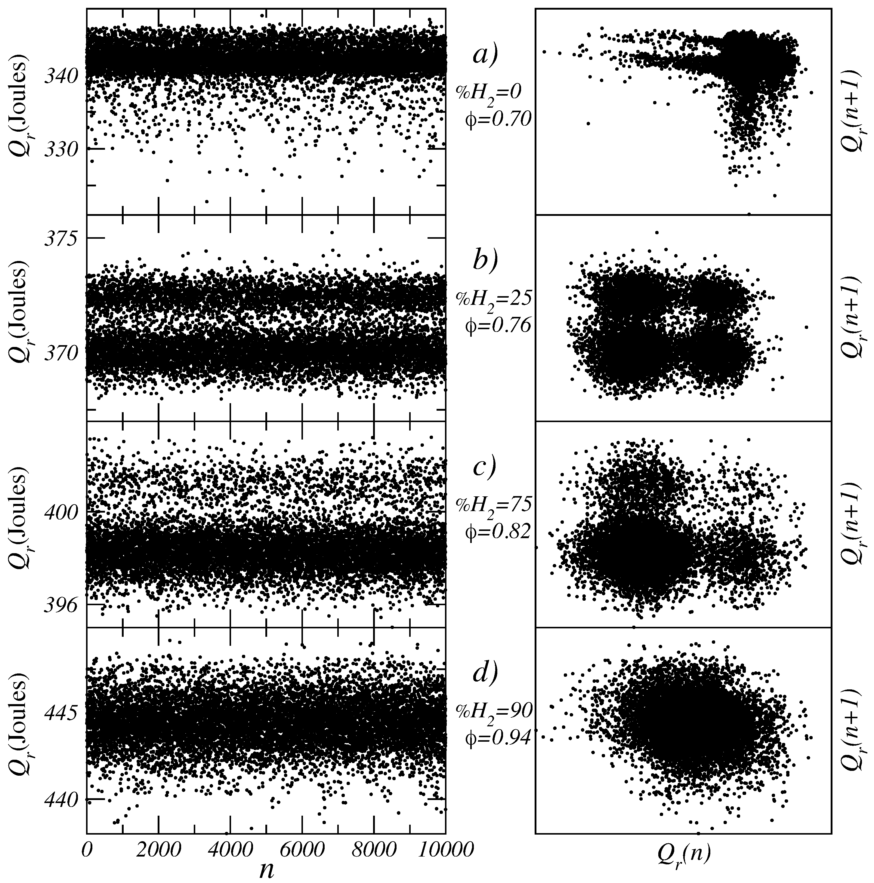
3. Simulated Heat Release Time Series

In regards to the calculation of the heat release from the outlined computer simulation model, it is convenient to recall that the thermodynamic efficiency of the engine at certain operating conditions is the ratio of the net work produced per cycle to the energy supplied, η = W / Q r , where Q r is the energy released by the fuel in the combustion process. By applying the first principle of thermodynamics to open systems, the heat release during combustion, δ Q r , can be calculated in terms of variations of internal energy associated with temperature changes, d U , the work output, δ W , and the heat transfer from the working fluid to the cylinder walls, δ Q s ,
δ Q r = d U + δ W + δ Q s
As mentioned before, Eichelberg’s correlation [39] is used to estimate Q s . Net heat release during the whole combustion process is calculated from the integration of heat release during that period. A detailed explanation can be found in [30,36].
As commented in the Introduction, quasi-dimensional simulations allow us to obtain CCV time series of any variable in the engine for several thousand of cycles with a not-too-expensive computational cost. This is difficult to do in experiments or CFD simulations. Hence, it is an adequate technique for the diagnosis of CCV in spark ignition engines, particularly in which respect to the existence of determinism or long time correlations. Heat release time series were computed for several fuel–air ratios, from lean to stoichiometric mixtures, and for different hydrogen concentrations per fuel volume, from pure isooctane ( % H 2 = 0 ) to pure hydrogen ( % H 2 = 100 ). In all cases, time series were obtained for 10 4 cycles. These time series are depicted in Figure 3. The plot is divided in sections, each for a particular fuel–air ratio, ϕ , and for several values of hydrogen concentration, % H 2 . It is observed that the mean value of Q r increases when ϕ increases from 0.7 to 1.0 , whereas for a specific value of ϕ , it is apparent that the mean value of Q r decreases with increasing hydrogen concentration. To understand this point, it is noteworthy that the energy density of hydrogen on a volume basis is much lower than that of gasoline. For this type of fuel the air displacement due to the gaseous state of hydrogen at inlet conditions results in a low volumetric efficiency and a loss of performance. Therefore, many hydrogen-powered engines suffer a lower heat release. This effect is clear in Figure 3 where for all fuel–air ratios the heat release decreases with increasing concentration of H2 and becomes minimal for % H 2 = 100 . Thus, using a small amount of hydrogen as an additive to hydrocarbon-fueled engines could maintain the positive properties of isooctane, avoiding harmful power losses. Different levels of CCV dispersion are observed in Figure 3.
The computed mean values of Q r vs. % H 2 for each fuel–air ratio, ϕ , are plotted in Figure 4a. As mentioned above, it is clear that as the fuel–air ratio increases, the mean value of Q r increases nregardless of the value of % H 2 concentration. In addition, it is also observed that the mean value of Q r is almost constant for a wide range of hydrogen concentrations. When % H 2 80 , a rapid reduction is observed in all cases, independently of ϕ . Similar behavior has been recently found for engine power output [31].
Next, the coefficient of variation COV (defined as C O V = σ / μ , where σ is the standard deviation and μ the mean of the sequence) for heat release sequences, Q r , is analyzed. This key statistical parameter gives information of the amplitude of the variability of a time series with respect to the mean value. In Figure 4b the COV of Q r for all fuel–air ratios and hydrogen concentrations is presented. The evolution in terms of hydrogen concentration is not clear. For each fuel–air ratio there appears to be a decrease from % H 2 = 0 up to a minimum value, in the range 70 % H 2 90 , although this depends on ϕ . It is remarkable that no clear conclusions can be extracted from the analysis of COV trends. Recently, the evolution of the COV of a different parameter, the power output, with fuel–air ratio and hydrogen concentration was reported [31]. For power output, the evolution of the COV is more straightforward. It is larger for lean mixtures, as expected. For % H 2 = 0 it has a relatively high value for any value of ϕ . Then, it decreases as hydrogen concentration increases (for any fixed ϕ ) and shows a minimum that depends on the fuel–air ratio. Afterwards, it increases when approaching % H 2 = 100 . This final increase could be associated to the fact that the spark advance was always kept constant (as it was done in the experimental work by Ji et al. [8]), and it was not tuned for each fuel–air ratio and hydrogen concentration combination. Hence, the evolution of the COV should be understood in this context.
In Figure 5, four representative cases of the time series of heat release and the corresponding first return maps are shown in detail. These examples us allow to identify several types of dynamics. For a lean mixture and pure isooctane fueling (Figure 5a, left) a main occupation region with sparse fluctuations in downwards direction is observed. The corresponding return maps (right) exhibit a boomerang-shaped structure. For a lean mixture with 25% hydrogen in volume, two densely populated regions are apparent (Figure 5b) . The corresponding return map shows a four-region structure indicating that the system stays for more than two cycles in the same state. The third case depicted in (Figure 5c) shows an evolution towards a single state. In Figure 5d it is observed that the dynamics become more homogeneous, alternating around a main state, as can be observed in the corresponding return map where an unstructured cloud of dots is perceived. To go further in the analysis of the heat release signals, symbol statistical techniques will be employed.

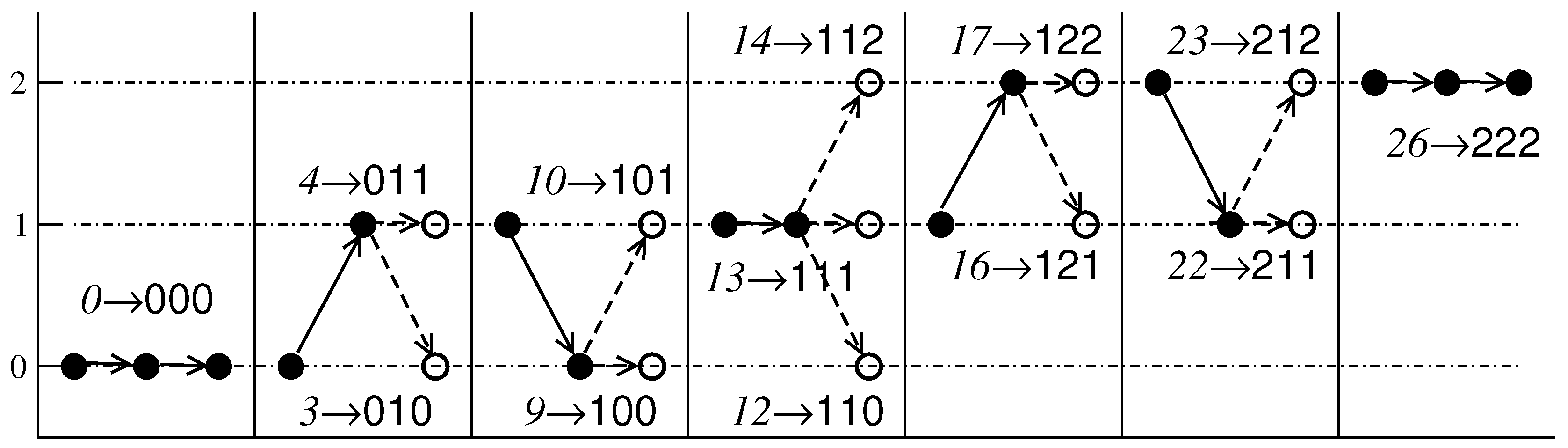
4. Symbolic Analysis Framework

A number of symbol statistic techniques have been used for different but equivalent purposes: to extract information on high-dimensional dynamics hidden in low-dimensional time series observations [19,32,33,34]. Many of them, especially when applied to combustion engine variability, consist of the construction of an alphabet of n symbols obtained from the original time series by generating a discrete partition of n regions. A particular symbol value is assigned to each one [24,25,26,27]. As mentioned in [19], there are main two procedures for selecting partitions: equiprobable partitions, where each partition has the same probability of appearance, and equispatial partitions, based on the division of intervals of the signal range. In the last case, rare events are easier to detect. In addition, to identify temporal patterns in the time series once it is symbolized, the joint probability of occurrence of L consecutive symbols, often called word, is analyzed. To generate these words a window of L symbols slides along the whole symbolized sequence in one-symbol steps. The total number of words of length L for an alphabet of n symbols is N = n L . It is also useful to evaluate the equivalent b a s e 10 value (or code) for n , L symbol-encoding. For example, if n = 2 (binary partition) and L = 4 , encoding results in N = 2 4 = 16 words. As an example, a particular sequence or word 1101 has an equivalent decimal code of 13. The number of symbols to assign and the length of the word structure L depends on the structure of the data to be analyzed.
An alternative way to choose the optimal value of L is based on the measure of uncertainty given by the well-known Shannon entropy [32],
H s ( L ) = 1 l o g ( N ) i p i ( L ) log p i ( L ) ,
where N is the total number of symbol sequences with non-zero probability, and p i ( L ) is the probability of a given sequence pattern. For truly random data, H s should equal 1, whereas for non-random (more deterministic) data, 0 < H s < 1 . More precisely, entropy is the mean rate of information production or how much new information is produced on average for each new element of the sequence; when more regularity is present, the entropy value is low, while high irregularity leads to H s = 1 .
In the previous section, several particular types of dynamics were described, roughly characterized by the shape of their return maps (see Figure 5). From such information n = 3 is chosen to describe the dynamics among the three regions mentioned above. The symbol regions are generated by constructing three equal size gaps between minimum and maximum values of the time series. The symbol 0 is assigned for the bottom region, the symbol 1 for the intermediate one, and the symbol 2 for the top one (see Figure 6). The return maps shown in Figure 5 also suggest that to take a length word, L = 3 , since three consecutive states give information about transitions in these. Later on, it will be shown that this partition is adequate to describe these behaviors. The analysis of three consecutive states gives us the possibility to study the permanence in a particular region, or two types of transitions: soft transitions, between two neighbor states, or wild transitions, among the three regions. Soft transitions are better explained in Figure 7. The cases depicted correspond to the most significant codes in symbol sequence that will be later analyzed.

5. Discussion of Symbolic Analysis Findings

Before discussing the results obtained for Q r , three random processes as a framework to compare noisy dynamics with those coming from deterministic structures are analyzed. These processes, depicted in the left side of Figure 8 (and their corresponding return maps on the right side), mimic the occupation shapes observed in simulations: first, a random process arising from a log-normal distribution, which generates sparse large fluctuations in one direction (see Figure 8a,b); second, a period-2 logistic map with Gaussian noise added to the feedback parameter, as an example of a process with three well defined regions and a poorly occupied central state (see Figure 8c,d); and third, a purely white noise sequence, as an example of uncorrelated process with a highly populated central state (see Figure 8e,f).
The pattern structure is analyzed by plotting symbol sequence histograms (SSHs). These are constructed with a horizontal axis corresponding to a specific symbol sequence code and a vertical axis with the relative frequency of the occurrence of each code. In Figure 9 it is observed that, for n = 3 and L = 3 , white noise exhibits a symmetric structure, centered in the code 13 (that corresponds to 111, which means that no variability is observed and the middle region is the most populated). The other words that are most frequent in white noise are 4(011), 10(101), 16(121), and 22(211). In all of them it is observed that the final state is 1, i.e., in spite of changes to another state, the sequence mainly prefers to return to the central region (or to remain in it) . On the other hand, the noisy logistic map exhibits a clearly unpopulated central state ( 13 c o d e ) and no symmetry is observed. Moreover, there are specific sequences which denote wild transitions between regions, as is the case of codes 6(020), 7(021), 15(120), and 20(202); or intermittency between middle and top region (codes 16(121) and 23(212)). These observations clearly describe the nature of the 2-period noisy logistic map used to generate the signals. Finally, log-normal noise is only significant at code 26(111), that is, there exists a preference to occupy the top state.
Here we review the symbolic analysis of the simulated heat release time series. First, Shannon entropy, H s , calculations are shown in order to select an appropriate word length, L. In Figure 10 the trends of H s vs. L for all the cases of % H 2 and for two fuel–air ratio values ( ϕ = 0.76 and ϕ = 0.94 ) are depicted. The values of H s are sensitive to the variations of % H 2 in both cases. For small values of L, H s decreases as the concentration of % H 2 increases, except for the case % H 2 = 100 and ϕ = 0.76 . These decrements in H s can be identified as an increment in the regularity and hence, as a signature of the existence of non-random structures. For large values of L, H s has a clear tendency to increase towards the value 1, indicating that the irregularity is high. The value L = 3 is an appropriate one, because it gives an stable value of H s , just before H s starts to increase for most combinations of fuel–air ratio and hydrogen concentration. The election of a larger value for L would imply a higher H s without gaining more relevant information about the permanence or intermittency among states. Hence, in this paper L = 3 is taken in order to study the particular behavior observed in the simulations for heat release sequences for different values of blended fuel–air ratio ϕ and hydrogen concentrations, % H 2 .
In Figure 11a the results of SSHs for different values of % H 2 and a lean mixture, ϕ = 0.76 are presented. Hydrogen concentrations that display qualitatively similar patterns have been grouped. This classification leads to two sets, % H 2 50 and % H 2 > 50 . All the curves, independently of % H 2 , present a common feature: relative frequencies are asymmetric with respect to the central code 13 (corresponding to 111, see Figure 7). For % H 2 50 (solid lines in Figure 11a) frequency peaks only exist in codes below 13 and those above are poorly populated. This means that transitions are associated to decays from the mean value of Q r to cycles with poor heat release or reverse. The most populated sequences are 0 (corresponding to 000), 4 (011), 10 (101), and 13 (111). All of them correspond to soft transitions (only two states are involved) and are similar to white noise (see Figure 9). However, in white noise, peaks are symmetric with respect to code 13 and the peak at 0 does not exist. For % H 2 > 50 , frequency peaks appear for codes over 13, so there are jumps from the mean value of Q r to larger heat release cycles. The most populated codes are 16 (121), 22 (211), and 26 (222). Again, all of them are soft transitions that are present in white noise except 26.
For a fuel mixture with fuel–air ratio close to stoichiometric conditions ( ϕ = 0.94 , Figure 11b) the grouping in terms of % H 2 is more subtle. Hydrogen concentrations that present similar histograms are shown in Figure 11b. Solid lines correspond to % H 2 = 0 , 25, and 100. The comments above for ϕ = 0.76 and % H 2 50 apply in this case. In the rest of cases (dashed lines), distribution of populations is similar to % H 2 > 50 in Figure 11a. Hence, for a relatively high fuel–air ratio the evolution with hydrogen concentration is not as straightforward as for lean mixtures. An interesting difference between lean and stoichiometric mixtures is that in the latter the codes 0 and 26 (the extremes) are infrequent.
In Figure 12 the frequency profiles of the codes for all the values of % H 2 are shown. For ϕ = 0.76 the distribution of frequencies exhibits three regions in terms of % H 2 . Very low hydrogen concentrations lead to a uniform frequency distribution without peaks. For % H 2 of approximately between 25 and 70, low frequencies are apparent for high codes and there are frequency peaks for codes below 13, corresponding to soft transitions as shown above. For higher % H 2 the behavior is opposite; now frequency peaks appear for codes over 13, and frequencies are uniform and low for codes below 13. For ϕ = 0.96 (right plot on Figure 12), a similar analysis can be done. Now the plot shows uniform cold regions for codes below 13 at high % H 2 and above 13 at low % H 2 . The most populated code is 13 and there are asymmetric peaks on the other regions.
In Figure 13 the SSHs for different values of ϕ are plotted. Again, the absence of wild transitions is remarkable. Three specific hydrogen concentrations are depicted. In Figure 13a, with % H 2 = 25 , no variability codes are as significant as soft transitions codes in most of the cases. Only in the case of ϕ = 0.7 is evidence of boomerang dynamics observed, indicating that for lean mixture of ϕ and low % H 2 the dynamics are significantly unstable. Also, remarkable asymmetry is present mainly in Figure 13a,b. This is associated to a two-state intermittency, as was previously discussed for the noisy logistic map process. This asymmetry tends to disappear in Figure 13c, with % H 2 = 90 indicating more regularity in the central region with uncorrelated variability, as discussed above for white noise behavior. Also, when % H 2 is increased in Figure 13b,c, a central code 13 arises. This is indicative of reduction of variability when hydrogen concentration is increased. The case ϕ = 0.7 , % H 2 = 90 resembles to a high extent the pattern of white noise (see Figure 9). Figure 14 gives a whole picture of the frequency distribution in terms of ϕ and % H 2 .
From Figure 11 and Figure 13, it is evident that only soft transitions are significant in the evolution for all cases. In contrast with the reduction of variability, a Gaussian random behavior emerges when ϕ is close to stoichiometric conditions, leading to more stable but less predictable dynamics.

6. Summary and Conclusions

A study to evaluate the effect of the addition of hydrogen to isooctane in a spark ignition engine with respect to cycle-to-cycle variability has been presented. Long heat release time series ( 10 4 cycles) obtained from a quasi-dimensional simulation scheme were built and analyzed. First-order return maps were plotted and compared with standard noises. Heat release first return maps present a wide variety of patterns depending on the blended fuel–air ratio and on the hydrogen concentration: boomerang-shaped structures were associated to a highly populated region and frequent cycles with poor heat release, three- or four-pole patterns were associated to two dense regions and transitions between them, and unstructured spots were associated to a central region with symmetric fluctuations below or above. In order to explore the presence of determinism in the signals and to quantify its regularity, Shannon entropy and symbol sequence analyses were performed. Shannon entropy calculations allowed us to establish the adequate codes and word length. However, conclusions from Shannon entropy calculations may lead to the notion that when observing the evolution of heat release on a larger scale, the variations seem to be more regular as the % H 2 is increased, i.e., a few patterns tend to dominate the dynamics.
However, the local behavior (represented by the symbolic patterns and quantified by their relative frequency) reveals that as the hydrogen concentration is increased, a number of different configurations of dominant patterns take place, which clearly differ from the white noise dynamics. Symbol sequence histograms confirm the presence of non-random structure in the dynamics for all hydrogen concentrations. Globally, all realizations present signs of non-variability in three consecutive states, or preferred transitions with neighbor states (soft transitions). Moreover, increasing % H 2 promotes a change of the dynamics from boomerang and two-state behaviors to more uniform one-band uncorrelated random dynamics with signs of regularity. These findings confirm the presence of predictable patterns and the usefulness of symbol sequence analysis in order to develop cyclic variability control strategies.

Acknowledgments

Alejandro Medina and Antonio Calvo Hernandez acknowledge financial support from JCyL of Spain, grant SA017P17. Lev Guzman-Vargas and Israel Reyes-Ramírez acknowledge COFAA-IPN , EDI-IPN, and SNI-CONACyT, México, and give special thanks to CSL-UPIITA. This work was carried out during the sabbatical leave of Israel Reyes-Ramírez at Departamento de Física Aplicada, Facultad de Ciencias, USAL. Santiago D. Martinez-Boggio and Pedro L. Curto-Risso acknowledge support from Universidad de la República and Agencia Nacional de Investigación e Innovación, Uruguay.

Author Contributions

Israel Reyes-Ramírez and Lev Guzman-Vargas performed the numerical calculations with reference to the symbolic analysis and wrote the corresponding sections; Santiago D. Martinez-Boggio and Pedro L. Curto-Risso designed and ran the spark engine simulations; and Alejandro Medina and Antonio Calvo Hernandez conceived the main lines of the research and wrote part of the manuscript.

Conflicts of Interest

The authors declare no conflict of interest.

References

  1. Al-Durra, A.; Canova, M.; Yurkovich, S. A real-time pressure estimation algorithm for closed-loop combustion control. Mech. Syst. Signal Process. 2013, 38, 411–427. [Google Scholar] [CrossRef]
  2. Maurya, R.K.; Pal, D.D.; Agarwal, A.K. Digital signal processing of cylinder pressure data for combustion diagnostics of HCCI engine. Mech. Syst. Signal Process. 2013, 36, 95–109. [Google Scholar] [CrossRef]
  3. Karim, G.A. Hydrogen as a spark ignition engine fuel. Int. J. Hydrogen Energy 2003, 28, 569–577. [Google Scholar] [CrossRef]
  4. White, C.M.; Steeper, R.R.; Lutz, A.E. The hydrogen-fueled internal combustion engine: A technical review. Int. J. Hydrogen Energy 2006, 31, 1292–1305. [Google Scholar] [CrossRef]
  5. Verhelst, S.; Wallner, T. Hydrogen-fueled internal combustion engines. Prog. Energy Combust. Sci. 2009, 35, 490. [Google Scholar] [CrossRef]
  6. D’Andrea, T.; Henshawa, P.F.; Tingb, D.S.-K. The addition of hydrogen to a gasoline-fuelled SI engine. Int. J. Hydrogen Energy 2004, 29, 1541–1552. [Google Scholar] [CrossRef]
  7. Ji, C.; Wang, S. Effect of hydrogen addition on the idle performance of a spark ignited gasoline engine at stoichiometric condition. Int. J. Hydrogen Energy 2009, 34, 3546–3556. [Google Scholar] [CrossRef]
  8. Ji, C.; Wang, S. Effect of hydrogen addition on combustion and emissions performance of a spark ignition gasoline engine at lean conditions. Int. J. Hydrogen Energy 2009, 34, 7823–7834. [Google Scholar] [CrossRef]
  9. Ji, C.; Wang, S.; Zhang, B. Effect of spark timing on the performance of a hybrid hydrogen-gasoline engine at lean conditions. Int. J. Hydrogen Energy 2010, 35, 2203–2212. [Google Scholar] [CrossRef]
  10. Wang, S.; Ji, C.; Zhang, B.; Liu, X. Realizing the part load control of a hydrogen-blended gasoline engine at the wide open throttle condition. Int. J. Hydrogen Energy 2014, 39, 7428–7436. [Google Scholar] [CrossRef]
  11. Wang, S.; Ji, C.; Zhang, B.; Liu, X. Lean burn performance of a hydrogen-blended gasoline engine at the wide open throttle condition. Appl. Energy 2014, 136, 43–50. [Google Scholar] [CrossRef]
  12. Ji, C.; Liu, X.; Gao, B.; Wang, S.; Yang, J. Numerical investigation on the combustion process in a spark-ignition engine fueled with hydrogen-gasoline blends. Int. J Hydrogen Energy 2013, 38, 11149–11155. [Google Scholar] [CrossRef]
  13. Ji, C.; Liu, X.; Wang, S.; Gao, B.; Yang, J. Development and validation of a laminar flame speed correlation for the CFD simulation of hydrogen-enriched gasoline engines. Int. J. Hydrogen Energy 2013, 38, 1997–2006. [Google Scholar] [CrossRef]
  14. Sen, A.; Longwic, R.; Litak, G.; Gorski, K. Analysis of cycle-to-cycle pressure oscillations in a diesel engine. Mech. Syst. Signal Process. 2008, 22, 362–373. [Google Scholar] [CrossRef]
  15. Roberts, J.B.; Peyton Jones, J.C.; Landsborough, K.J. Stochastic modelling and estimation for cyclic pressure variations in spark ignition engines. Mech. Syst. Signal Process. 2001, 15, 419–438. [Google Scholar] [CrossRef]
  16. Martínez, S.; Irimescu, A.; Merola, S.S.; Lacava, P.; Curto-Risso, P.L. Flame front propagation in an optical GDI engine under stoichiometric and lean burn conditions. Energies 2017, 10, 1337. [Google Scholar]
  17. Srivastav, A.; Ray, A.; Gupta, S. An information-theoretic measure for anomaly detection in complex dynamical systems. Mech. Syst. Signal Process. 2009, 23, 358–371. [Google Scholar] [CrossRef]
  18. Wagner, R.M.; Drallmeier, J.A.; Daw, C.S. Prior-Cycle Effects in Lean Spark Ignition Combustion-Fuel/Air Charge Considerations; SAE Paper 981047; SAE International: Warrendale, PA, USA, 1998. [Google Scholar]
  19. Finney, C.E.; Kaul, B.C.; Daw, C.S.; Wagner, R.M.; Edwards, K.D.; Green, J.B., Jr. Invited review: A review of deterministic effects in cyclic variability of internal combustion engines. Int. J. Engine Res. 2015, 16, 366–378. [Google Scholar] [CrossRef]
  20. Sen, A.K.; Litak, G.; Finney, C.E.A.; Daw, C.S.; Wagner, R.M. Analysis of heat release dynamics in an internal combustion engine using multifractals and wavelets. Appl. Energy 2010, 87, 1736–1743. [Google Scholar] [CrossRef]
  21. Ma, F.; Li, S.; Zhao, J.; Qi, Z.; Deng, J.; Naeve, N.; He, Y.; Zhao, S. A fractal-based quasi-dimensional combustion model for SI engines fuelled by hydrogen enriched compressed natural gas. Int. J. Hydrogen Energy 2012, 37, 9892–9901. [Google Scholar] [CrossRef]
  22. Curto-Risso, P.L.; Medina, A.; Calvo Hernández, A.; Guzmán-Vargas, L.; Angulo-Brown, F. Monofractal and multifractal analysis of simulated heat release fluctuations in a spark ignition heat engine. Physica A 2010, 389, 5662–5670. [Google Scholar] [CrossRef]
  23. Sen, A.K.; Medina, A.; Curto-Risso, P.L.; Calvo Hernández, A. Effect of ethanol addition on cyclic variability in a simulated spark igntion engine. Meccanica 2014, 49, 2285–2297. [Google Scholar] [CrossRef]
  24. Daw, C.S.; Kennel, M.B.; Finney, C.E.A.; Connolly, F.T. Observing and modeling nonlinear dynamics in an internal combustion engine. Phys. Rev. E 1998, 57, 2811–2819. [Google Scholar] [CrossRef]
  25. Ghazimirsaied, A.; Shahbakhti, M.; Koch, C.R. HCCI engine combustion phasing prediction using a symbolic-statistics approach. J. Eng. Gas Turbines Power 2010, 132, 082805. [Google Scholar] [CrossRef]
  26. Ghazimirsaied, A.; Koch, C.R. Controlling cyclic combustion timing variations using a symbol-statistics predictive approach in an hcci engine. Appl. Energy 2012, 92, 133–146. [Google Scholar] [CrossRef]
  27. Chen, Y.; Dong, G.; Mack, J.H.; Butt, R.H.; Chen, J.Y.; Dibble, R.W. Cyclic variations and prior-cycle effects of ion current sensing in an hcci engine: A time-series analysis. Appl. Energy 2016, 168, 628–635. [Google Scholar] [CrossRef]
  28. Li, F.; Wang, H.; Zhou, G.; Yu, D.; Li, J.; Gao, H. Anomaly detection in gas turbine fuel systems using a sequential symbolic method. Energies 2017, 10, 724. [Google Scholar] [CrossRef]
  29. Curto-Risso, P.L.; Medina, A.; Calvo Hernández, A. Optimizing the geometrical parameters of a spark ignition engine: Simulation and theoretical tools. Appl. Therm. Eng. 2011, 31, 803–810. [Google Scholar] [CrossRef]
  30. Curto-Risso, P.L.; Medina, A.; Calvo Hernández, A.; Guzmán-Vargas, L.; Angulo-Brown, F. On cycle-to-cycle heat release variations in a simulated spark ignition heat engine. Appl. Energy 2011, 88, 1557–1567. [Google Scholar] [CrossRef]
  31. Martínez-Boggio, S.; Curto-Risso, P.L.; Medina, A.; Calvo Hernández, A. Simulation of cycle-to-cycle variations on spark ignition engines fueled with gasoline-hydrogen blends. Int. J. Hydrogen Energy 2016, in press. [Google Scholar]
  32. Tang, X.Z.; Tracy, E.R.; Boozer, A.D.; Brown, R. Symbol sequence statistics in noisy chaotic signal reconstruction. Phys. Rev. E 1995, 51, 3871. [Google Scholar] [CrossRef]
  33. Daw, C.S.; Finney, C.E.A.; Kennel, M.B. Symbolic approach for measuring temporal irreversibility. Phys. Rev. E 2000, 62, 1912–1921. [Google Scholar] [CrossRef]
  34. Daw, C.S.; Finney, C.E.A.; Tracy, E.R. A review of symbolic analysis of experimental data. Rev. Sci. Instrum. 2003, 74, 915–930. [Google Scholar] [CrossRef]
  35. Curto-Risso, P.L.; Medina, A.; Calvo Hernández, A. Optimizing the operation of a spark ignition engine: Simulation and theoretical tools. J. Appl. Phys. 2009, 105, 094904. [Google Scholar] [CrossRef]
  36. Medina, A.; Curto-Risso, P.L.; Calvo Hernández, A.; Guzmán-Vargas, L.; Angulo-Brown, F.; Sen, A.K. Quasi-Dimensional Simulation of Spark Ignition Engines; Springer: Berlin, Germany, 2014. [Google Scholar]
  37. Heywood, J.B. Internal Combustion Engine Fundamentals; McGraw-Hill: New York, NY, USA, 1988; Appendix C; p. 906. [Google Scholar]
  38. Barnes-Moss, H.W. A Designer’s Viewpoint in Passenger Car Engines, Conference Proceedings; Institution of Mechanical Engineers: London, UK, 1975; pp. 133–147. [Google Scholar]
  39. Eichelberg, G. Some new investigations on old combustion-engine problems. Engineering 1939, 148, 463–547. [Google Scholar]
  40. Bayraktar, H.; Durgun, O. Mathematical modeling of spark-ignition engine cycles. Energy Sources 2003, 25, 439–455. [Google Scholar] [CrossRef]
  41. Blizard, N.C.; Keck, J.C. Experimental and Theoretical Investigation of Turbulent Burning Model for Internal Combustion Engines; SAE Paper 740191; SAE International: Warrendale, PA, USA, 1974. [Google Scholar]
  42. Beretta, G.P.; Rashidi, M.; Keck, J.C. Turbulent flame propagation and combustion in spark ignition engines. Combust. Flame 1983, 52, 217–245. [Google Scholar] [CrossRef]
  43. Heywood, J.B. Combustion and its modeling in spark-ignition engines. In Proceedings of the International Symposium (COMODIA), Yokohama, Japan, 11–14 July 1994; Volume 94. [Google Scholar]
  44. Heywood, J.B. Internal Combustion Engine Fundamentals; McGraw-Hill: New York, NY, USA, 1988; Chapter 14; pp. 771–773. [Google Scholar]
  45. Metghalchi, M.; Keck, J.C. Laminar burning velocity of propane-air mixture at high temperature and pressure. Combust. Flame 1980, 38, 143. [Google Scholar] [CrossRef]
  46. Metghalchi, M.; Keck, J.C. Burning velocities of mixtures of air with methanol, isoctane, and indolene at high pressure and temperature. Combust. Flame 1982, 48, 191–210. [Google Scholar] [CrossRef]
  47. Heywood, J.B. Internal Combustion Engine Fundamentals; McGraw-Hill: New York, NY, USA, 1988; Chapter 9; pp. 413–427. [Google Scholar]
  48. Mandilas, C.; Ormsby, M.P.; Sheppard, C.G.W.; Woolley, R. Effects of hydrogen addition on laminar and turbulent premixed methane and iso-octane-air flames. Proc. Combust. Inst. 2007, 31, 1443–1450. [Google Scholar] [CrossRef]
  49. Emadi, M.; Karkow, D.; Salamesh, T.; Gohil, A.; Raterner, A. Flame structure changes resulting from hydrogen-enrichment and pressurization for low swirl premixed methane-air flames. Int. J. Hydrogen Energy 2012, 37, 10397–10404. [Google Scholar] [CrossRef]
  50. Ferguson, C.R. Internal Combustion Engines, Applied Thermosciences; John Wiley & Sons: Hoboken, NJ, USA, 1986. [Google Scholar]
  51. Irimescu, A.; Merona, S.S.; Valentino, G. Application of an entrainment turbulent combustion model with validation based on the distribution of chemical species in an optical spark ignition engine. Appl. Energy 2016, 162, 908–923. [Google Scholar] [CrossRef]
  52. Ma, F.; Wang, Y.; Wang, M.; Liu, H.; Wang, J.; Dinbg, S.; Zhao, S. Development and validation of a quasi-dimensional combustion model for SI engines fuelled by HCNG with variable hydrogen fractions. Int. J. Hydrogen Energy 2008, 33, 4863–4875. [Google Scholar] [CrossRef]
  53. Abdi Aghdam, E.; Burluka, A.A.; Hattrell, T.; Liu, K.; Sheppard, G.W.; Neumeister, J.; Crundwell, N. Study of Cyclic Variation in an SI Engine Using Quasi-Dimensional Combustion Model; SAE Paper 2007-01-0939; SAE International: Warrendale, PA, USA, 2007. [Google Scholar]
  54. Ozdor, N.; Dulger, M.; Sher, E. Cyclic Variability in Spark Ignition Engines. A Literature Survey; SAE Paper 940987; SAE International: Warrendale, PA, USA, 1994. [Google Scholar]
  55. Heywood, J.B.; Keck, J.C.; Beretta, G.P.; Watts, P.A. Combustion and Operating Characteristics of Spark-Ignition Engines; Technical Report; Massachusetts Institute of Technology: Cambridge, MA, USA, 1980. [Google Scholar]
  56. Wang, S.; Ji, C.; Zhang, B. Starting a spark-ignited engine with the gasoline-hydrogen mixture. Int. J. Hydrogen Energy 2011, 36, 4461–4468. [Google Scholar] [CrossRef]
Figure 1. Simulated coefficient of variation (COV) of indicated mean of effective pressure (IMEP) after 10 4 cycles (lines) and comparison with the experimental results of Ji et al. [56] (symbols). Three concentrations of hydrogen by volume are considered: H0 (pure isooctane), H71 (71% H2 by total fuel volume), and H85 (85%). Details can be checked in [31].
Energies 11 00968 g001
Figure 2. Plot of several cycles of in-cylinder pressure during combustion against crank angle (CA). Two hydrogen concentrations are shown, H0 and H71, for a fuel–air ratio ϕ = 0.79 . Thin lines represent individual simulated cycles; thick lines, average values (denoted as AVG); and symbols, experimental data [8].
Energies 11 00968 g002
Figure 3. Simulated heat release time series for different fuel–air ratios, ϕ , and hydrogen concentrations, % H 2 . Each case consists of 10,000 cycles.
Energies 11 00968 g003
Figure 4. (a) Evolution of the mean value of the heat release, Q r , vs. hydrogen concentration, % H 2 , for different fuel–air ratios, ϕ ; (b) Evolution of coefficient of variation (COV) for the same cases.
Energies 11 00968 g004
Figure 5. Representative cases of heat release sequences, x ( n ) (left side), and their corresponding first return maps (right side). (a) % H 2 = 0, ϕ = 0.70 ; (b) % H 2 = 25, ϕ = 0.76 ; (c) % H 2 = 75, ϕ = 0.82 ; (d) % H 2 = 90, ϕ = 0.94 .
Energies 11 00968 g005
Figure 6. Procedure for conversion of a time series to symbol series for a n = 3 partition.
Energies 11 00968 g006
Figure 7. Representative soft transitions in symbol sequences for n = 3 and L = 3 . Decimal sequence codes are shown in each case. This notation will be used in subsequent analysis.
Energies 11 00968 g007
Figure 8. Signals obtained from three different random processes ((a) Log-normal noise; (b) Noisy logistic map; (c) White noise) with their correspondent return maps ((d) Log-normal noise; (e) Noisy logistic map; (f) White noise).
Energies 11 00968 g008
Figure 9. Symbol sequence histograms (SSHs) for the random processes plotted in Figure 8, for n = 3 and L = 3 .
Energies 11 00968 g009
Figure 10. Evolution of the Shannon entropy, H s ( L ) , with the word length for two fuel–air ratios: (a) ϕ = 0.76 and (b) ϕ = 0.94 .
Energies 11 00968 g010
Figure 11. Symbol sequence histograms of the Q r sequence for all values of hydrogen concentrations for particular fuel ratios: (a) a lean mixture, ϕ = 0.76 ; (b) a close-to-stoichiometric one ϕ = 0.94 . Parameters for calculations are n = 3 , L = 3 .
Energies 11 00968 g011
Figure 12. Color density plots of symbol sequence histograms of Q r for the cases shown in Figure 11.
Energies 11 00968 g012
Figure 13. Symbol sequence histograms of Q r for several values of fuel–air ratio and particular hydrogen concentrations: (a) % H 2 = 25 , (b) % H 2 = 50 ; and (c) % H 2 = 90 . Parameters for calculations are n = 3 , L = 3 .
Energies 11 00968 g013
Figure 14. Frequency profiles of codes for all values for three hydrogen concentrations: (a) % H 2 = 25 ; (b) % H 2 = 50 ; and (c) % H 2 = 90 .
Energies 11 00968 g014
Table 1. Engine specifications [8] and operation parameters considered. ATDC applies for after top dead center and BTDC for before top dead center.
Engine TypeIn-Line, 4-Stroke
ManufacturerBeijing Hyundai Motors
Bore (mm)77.4
Stroke(mm)85
Connecting rod (mm)141
Displacement (L)1.599
Compression ratio10:1
Number of valves4 per cylinder
Manifold absolute pressure61.5 kPa
Spark advance (°CA BTDC)22
IVO (°CA BTDC)45
IVC (°CA BTDC)135
EVO (°CA ATDC)135
EVC (°CA ATDC)45
Rated torque (N.m/rpm)143/4500
Rated power (kW/rpm)82/6000
Engine speed (rpm)1400

