Carbon Debt Payback Time for a Biomass Fired CHP Plant—A Case Study from Northern Europe

Abstract

The European Union (EU) has experienced a large increase in the use of biomass for energy in the last decades. In 2015, biomass used to generate electricity, heat, and to a limited extent, liquid fuels accounted for 51% of the EU’s renewable energy production. Bioenergy use is expected to grow substantially to meet energy and climate targets for 2020 and beyond. This development has resulted in analyses suggesting the increased use of biomass for energy might initially lead to increased greenhouse gas (GHG) emissions to the atmosphere, a so-called carbon debt. Here, we analyze carbon debt and payback time of substituting coal with forest residues for combined heat and power generation (CHP). The analysis is, in contrast to most other studies, based on empirical data from a retrofit of a CHP plant in northern Europe. The results corroborate findings of a carbon debt, here 4.4 kg CO₂eq GJ⁻¹. The carbon debt has a payback time of one year after conversion, and furthermore, the results show that GHG emissions are reduced to 50% relative to continued coal combustion after about 12 years. The findings support the use of residue biomass for energy as an effective means for climate change mitigation.

1. Introduction

The recent decades, have seen a massive increase in the use of biomass for energy [1]. The majority of this increase has occurred in the European Union (EU), where bioenergy currently (2015) accounts for 51% of renewable energy production [2] and it is expected to increase further to meet the targets on renewable energy by 2020 [3,4]. A number of studies find that increased use of bioenergy creates a so-called carbon debt [5,6,7,8], which implies a period with larger greenhouse gas (GHG) emissions as compared to a continued fossil fuel use scenario. Assuming regrowth of harvested biomass, estimates of the payback time of this carbon debt have been as high as 400 years [9]. The implication of a carbon debt is that the contribution of bioenergy to climate change mitigation is delayed [10,11]. Buchholz et al. [12] conducted a meta-analysis of 59 carbon debt studies, and showed that the majority (47 studies) was based on hypothetical data and only a dozen were based on field data. Studies reporting long carbon debt payback times in general assume that the biomass is utilized for electricity production with low conversion efficiencies and that the woody biomass originates from the dedicated harvest of trees for energy from long rotation forestry [13]. Looking at the current use of bioenergy in the EU, there is little evidence that such supply chains dominate [14].

Data from EUROSTAT show that less than 1% of electricity production in the EU comes from solid biomass fired power plants [15]. Solid biomass is more prevalent in combined heat and power (CHP) and heat production that are plants feeding into district heating systems. 16.3% of heat production to district heating in the EU comes from solid biomass, while the majority comes from natural gas and coal [15]. Regarding the origin of the woody biomass used for bioenergy data are very sparse. Regarding wood chips, a survey by [14] found that the main source of wood chips for power and heat production in the EU was logging residues (36%) and whole trees from thinning operations (19%). Information from Drax power plant in the UK suggests similar sources [16]. These conclusions are in line with [3,17,18], who also estimate the current source of woody bioenergy as mainly wood waste, harvest residues, and thinnings. The objective of this study is to analyze the carbon dynamics involved in retrofitting a CHP plant from primarily coal firing to primarily wood firing, and to estimate the carbon debt payback time. Contrary to most other studies, which are based on hypothetical scenarios, this analysis benefits from the use of data from an existing power plant retrofit in northern Europe, which is considered to be representative for the use of biomass for CHP in the EU. This analysis is based on the carbon debt concept. Dehue [19] points out that there is no universally applied definition of ‘carbon debt’ and ‘carbon debt payback time’, leading authors to apply different definitions in an inconsistent manner. A definition often referred to is by Mitchell et al. [6], where the terms ‘carbon debt’, ‘carbon debt repayment’, and ‘carbon offset parity point’ are introduced. However, this definition only applies to bioenergy scenarios where the source of woody biomass comes from dedicated harvest and forest regrowth is included in the modelling. In contrast, bioenergy sources from wood waste and forest residues are resources that are generated independently of a bioenergy demand. The method that is used here is in line with the typical approach to carbon debt and payback time analyses [20], allowing for a comparison with other studies. In the following Section 2, we present the applied methodology, Section 3 presents the results of the analysis and their sensitivity to key assumptions. Section 4 discusses the findings relative to earlier research, leading to conclusions in Section 5.

2. Material and Methods

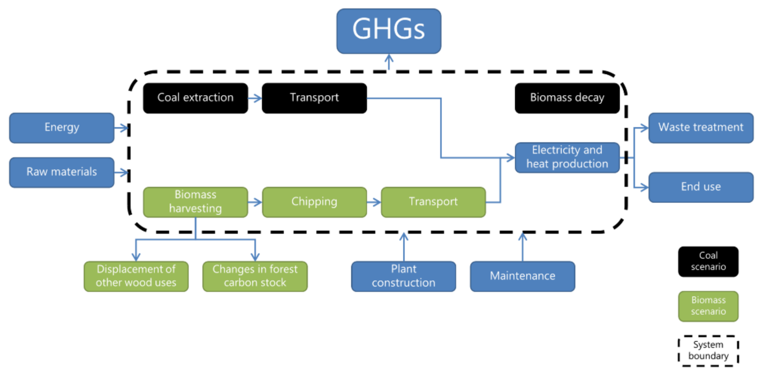
The analysis follows a life cycle inventory (LCI) approach quantifying the GHG emissions from both scenarios and ensuring comparability by using produced heat and electricity (1 GJ) as the common functional unit. The analysis estimates the global warming potential, and do not assess other environmental impacts, such as human toxicity, acidification, or resource depletion. The product system analyzed is illustrated in Figure 1.

The study covers the direct emissions from the extraction and processing, transportation and the combustion of the fuels. It therefore excludes the embodied emissions in the used fuels or materials, e.g., the emissions related to produce diesel used for transportation of biomass or coal. The system boundary also exclude emissions related to distribution and use of the produced heat and electricity together with emissions that are related to the end of life of the CHP plant. Furthermore, GHG emission related to indirect effects, e.g., indirect land use change or indirect wood use change, of biomass consumption are not considered.

The carbon debt concept is adopted from Mitchell et al. [6], but applied to waste and residue resources, as e.g., demonstrated by Sathre et al. [20] (Equation (1)).

$$NE=E_{bio}-\left(E_{fossil}+E_{decay}\right)$$

(1)

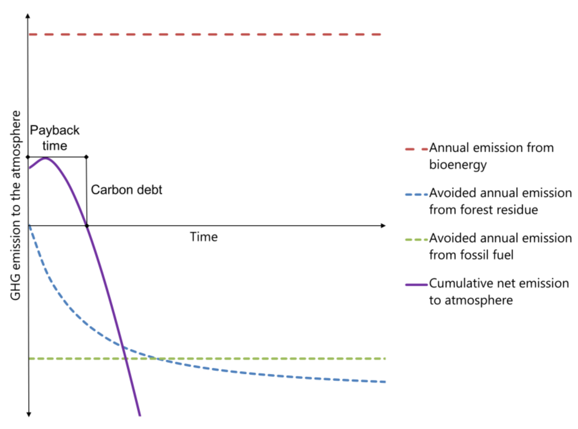
where NE is the annual net GHG emission to the atmosphere, E_bio is the direct GHG emissions from the bioenergy supply chain including emissions from biomass combustion, E_fossil the direct GHG emissions from the counterfactual fossil supply chain, including emissions from fossil fuel combustion, and E_decay the GHG emissions from the counterfactual decay of forest residues. The payback time is determined as the time, where the time integrated NE = 0. (Figure 2).

The conceptual carbon emission profile corresponds to modelled profiles for the use of stumps or branches for energy [20,21]. The payback time is understood as the point in time, where the bioenergy scenario starts to reduce the atmospheric GHG emissions relative to the counterfactual reference scenario. The combined heat and power (CHP) plant that is considered here is a medium sized Northern European utility feeding into a district heating network and the electricity grid. The plant has been converted from primarily coal firing to biomass firing, mainly wood chips. In retrofitting, the plant the boiler was replaced, while the rest of the plant needed little refurbishment. Detailed information about the plant has been anonymized on request. In contrast to assumptions applied by a number of other studies [6,7,22], the biomass scenario shows slightly higher fuel efficiency than the reference scenario, 85.9% as compared to 84.2%. Fuel efficiency is normalized with the power/heat ratio, which is influenced by different heat and electricity demands in 2005 and 2015. According to the head of production at the plant, the alternative to replacing the coal boiler with a biomass boiler would have been to keep the old coal boiler in operation and refurbish it.

Data regarding electricity and heat production has been acquired for the year 2015, where the plant was running exclusively on biomass along with data on the amount, type, and origin of the biomass fuel input. As reference scenario, the year 2005, where the plant was primarily firing coal, has been chosen. Had the plant not been converted into firing biomass, the existing coal boiler would likely have remained in place, with unchanged efficiencies and fuel inputs. It should be noted that during the conversion a flue gas condenser was installed to increase the overall efficiency of the plant. Heat production from this installation has been excluded from the 2015 data to ensure the comparability of general operation conditions between the two scenarios. As for 2015, the same data has been acquired for 2005.

The fuel inputs for 2005 (reference scenario) and for 2015 (biomass scenario) can be seen in

Table 1. Fuel inputs for the biomass year (2005) and the coal year (2015) based on energy content.

	Fuel Input 2005	Fuel Input 2015
	% (Based on Energy Content)
Coal	74.47	0.41
Wood chips		54.98
Wood logs		24.61
Wood pellets		10.88
Olive seeds	7.60
Other biomass	17.15	8.56
Meat and bone meal	0.17
Carbon residues	0.06
Land fill gas	0.56	0.57

. Regarding the reference scenario, the specifics concerning ‘Other biomass’, such as origin and type are not known. It is assumed that it shares the same characteristics as the biomass input in 2015. The other fuel inputs are all residue products, and therefore supply chain emissions that are related to forest harvest operations are omitted.

Unlike coal, biomass is delivered in many smaller batches with varying characteristics and are piled up in the storage area, from where they are fired into the boiler. Because of the varying quality of every batch (difference in water content) biomass from several batches are mixed and fired into the boiler to achieve the greatest reliability and consistency. The average storage time at the plant is about 1–2 months, which gives some overlap between years. Data on biomass delivery from 2014 has been acquired to normalize the 2015 data against the total biomass input. The ‘Other biomass’ fraction is made up of various waste products from different industries consuming woody biomass that is not suitable for other purposes. ‘Logs’ are delivered at the plant and then chipped and fired into the boiler.

Data available to estimate GHG emissions are the amounts delivered, energy content (carbon content for coal), and the origin of the fuel. The transport distance has been calculated with Google Maps for road transport and with online shipping distance tools for sea transport. Specific data on fuel use for transport, chipping, and harvesting were not available, and standard values from the Biograce II [23] GHG accounting tool were used to estimate GHG emissions from biomass processing and transportation. For emissions related to coal, data from the Ecoinvent LCI database [24] was used, which include all of the emissions related to the extraction of coal from different locations around the world. The GHGs included in the analysis are CO₂, CH₄ and N₂O with the GWP of 1, 28, and 265, respectively. Data are presented in

Table 2. GHG emission factors used in the study.

Process			Unit	GHG Emission	Reference
Transport	Bulk carrier		MJ (tonnes km)−1	0.24	Biograce II [23]
			g CO2eq MJ−1	93.3	Ibid
			g CO2eq (tonnes km)−1	22.39	Ibid
	Truck		MJ (tonnes km)−1	0.84	Ibid
			g CO2eq MJ−1	93.95	Ibid
			g CO2eq (tonnes km)−1	79.48	Ibid
Processing	Wood chips	Residue harvest	g CO2eq MJ−1 chips	1.48	Ibid
		Road transport (100 km)	g CO2eq MJ−1 chips	0.61	Ibid
		Chipping	g CO2eq MJ−1 chips	0.38	Ibid
		Total	g CO2eq MJ−1 chips	2.47	Ibid
	Logs	Harvest	g CO2eq MJ−1 chips	1.09	Ibid
		Road transport (100 km)	g CO2eq MJ−1 chips	0.61	Ibid
		Chipping	g CO2eq MJ−1 chips	0.38	Ibid
		Total	g CO2eq MJ−1 chips	2.08	Ibid
	Wood pellets	Total	g CO2eq MJ−1 pellets	17.99	Ibid
	Coal (origin)	Russia	kg CO2eq tonnes−1 coal	280	Ecoinvent [24]
		Canada	kg CO2eq tonnes−1 coal	865	Ibid
		Australia	kg CO2eq tonnes−1 coal	91	Ibid
		Central and eastern Europe	kg CO2eq tonnes−1 coal	233	Ibid
		Latin America	kg CO2eq tonnes−1 coal	30	Ibid
		North America	kg CO2eq tonnes−1 coal	99	Ibid
		Western Europe	kg CO2eq tonnes−1 coal	352	Ibid
		South Africa	kg CO2eq tonnes−1 coal	108	Ibid
		Mix	kg CO2eq tonnes−1 coal	207	Ibid
Combustion	Wood		kg CO2eq GJ−1 wood	113.9	IPCC [25]
	Coal		kg CO2eq GJ−1 coal	95	Ibid
	Land fill gas		kg CO2eq GJ−1 gas	54.7	Ibid

.

In order to set up a reference scenario, the realistic alternative use of the biomass must be determined. Based on a literature review and interview with some of the biomass suppliers to the plant, the most likely alternative is decomposition on the forest floor, either as logs or as branches. We use an exponential decay function, as described by Gustavsson et al. [26], to model the natural decay of biomass in the reference scenario:

$$M_t=M_o·e^{-kt}$$

(2)

M_o is the initial dry mass of organic matter, M_t is the remaining mass at time t and k is the decay constant. The decay constant can be described as a function of the half-life period of a mass:

$$k=\frac{\ln \left(2\right)}{l}$$

(3)

l is the half-life period.

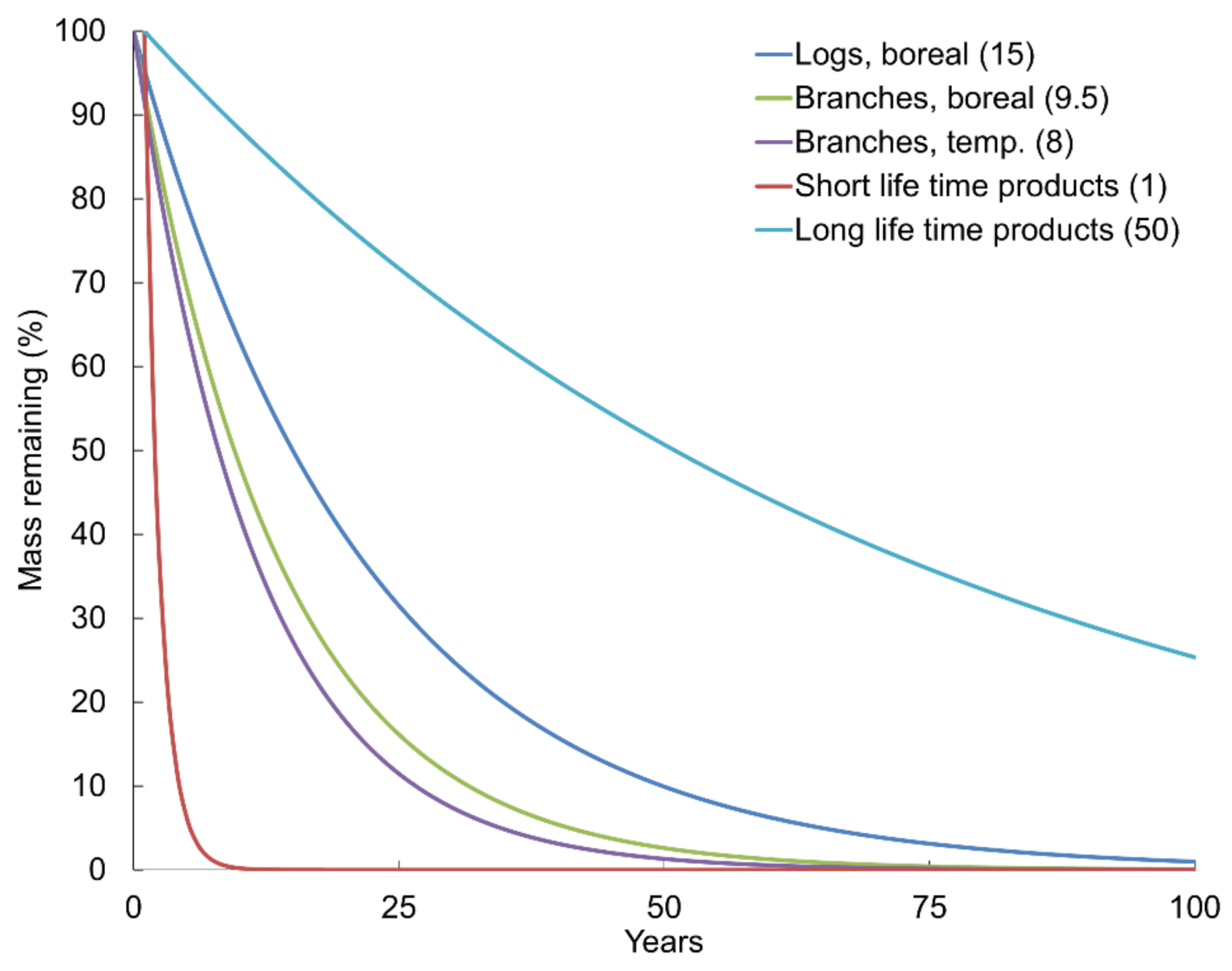
Figure 3 shows the decay rates for the different types of woody biomass used as fuel input, based on Gustavsson et al. [26]. They analyze a boreal forest system that is representative for most of the biomass supplied to the plant in the biomass scenario. Biomass is, however, also supplied from temperate forest ecosystems, which are assumed to have a higher decay rate. Using decay functions that were validated for boreal forest ecosystems on all biomass supplied to the plant represents a worst case scenario and avoids underestimation of carbon debt payback times. Slower natural decay rates of the biomass increases the payback time [13].

Other fuel inputs in the reference scenario, such as carbon residue and sawdust, are assumed to be used in various products. Carbon residue in the fly ash is a common additive in cement production, which is assumed to have a relatively long lifetime and in this analysis assigned a half-life period of 50 years. Other fuels, such as sawdust, which can be used as animal bedding and subsequently burned are assumed to have very short life times, and therefore assigned a half-life period of one year. These two types of fuels make up a marginal share of the total fuel consumption and do not have a significant impact on the overall GHG balance.

In both scenarios there is a relatively small input of landfill gas (<1%). Landfill gas is extracted from an old landfill and consists mainly of 55% methane (CH₄) and 35% carbon dioxide (CO₂). There are no alternative uses to landfill gas than burning it for energy production. If not used it would be emitted to the atmosphere as methane and CO₂. Since methane is a much more potent GHG than CO₂ (GWP of 28), there is a climate benefit from burning it. The avoided methane emissions have been converted into CO₂ equivalents and are subtracted from the final results.

Sensitivity Analysis

To test the robustness of the result, model parameters with the highest uncertainties are adjusted. Included in the sensitivity analysis is: (a) the decay rates (half-life periods) of biomass resources, (b) emissions factor for wood, and (c) the fuel efficiency of the plant (

Table 3. Parameters and parameter values included in the sensitivity analysis.

Parameters	Changes Relative to Base Case
Half-life of decaying biomass	50%, 200%, 400%
Emission factor of wood	−10%, +10%
Biomass fuel conversion efficiency	−10%
Coal fuel conversion efficiency	+10%

). The carbon content of the coal used in 2005 was known, allowing for accurate estimates of the CO₂ emissions from combustion. The carbon content of wood was not known, and therefore an average value of 113.9 kg CO₂eq GJ⁻¹ has been used as recommended in the IPCC Guidelines for National GHG Inventories [25]. The IPCC Guidelines furthermore emphasize that the emission factor of wood can vary considerably, and therefore contribute to inherent uncertainty. It was not considered meaningful to analyze changing emission factors for transportation and processing of the fuels, since their share of the overall emissions was relatively small.

3. Results

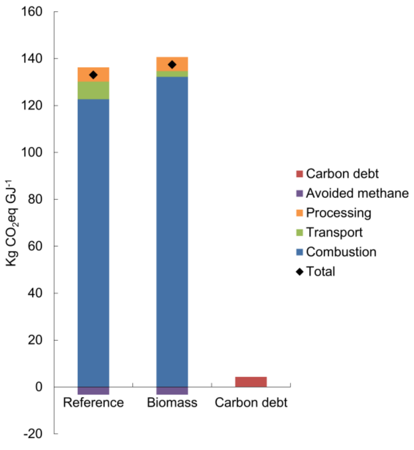
The total emissions per produced GJ are almost identical for both scenarios. Emissions from the biomass scenario are slightly higher by 4.4 kg CO₂eq GJ⁻¹, which represents the carbon debt, equaling 3.2% of the total emissions. Emissions from fuel combustion constitute the largest share with 92% in the reference scenario and 96% in the biomass scenario. Emissions from other sources than combustion, also referred to as supply chain emissions, constitute a minor share of the total emissions. The carbon debt more or less equals the emissions related to transportation in the biomass scenario. Figure 4 shows total CO₂eq emission per produced GJ allocated to combustion, processing and transportation. Avoided methane emissions from landfill gas have been included in both scenarios.

Emissions from processing are roughly identical for both scenarios; however, transport emissions are approximately three times higher in the reference scenario than the biomass scenario. This is in line with earlier research and is mainly attributable to longer transport distances for coal [11,27]. The carbon debt incurred in the transition from coal to biomass is primarily related to the higher carbon intensity of biomass when compared to coal due to a lower carbon to oxygen ratio in biomass. Lower supply chain emissions in the biomass scenario, on the other hand, reduces the carbon debt.

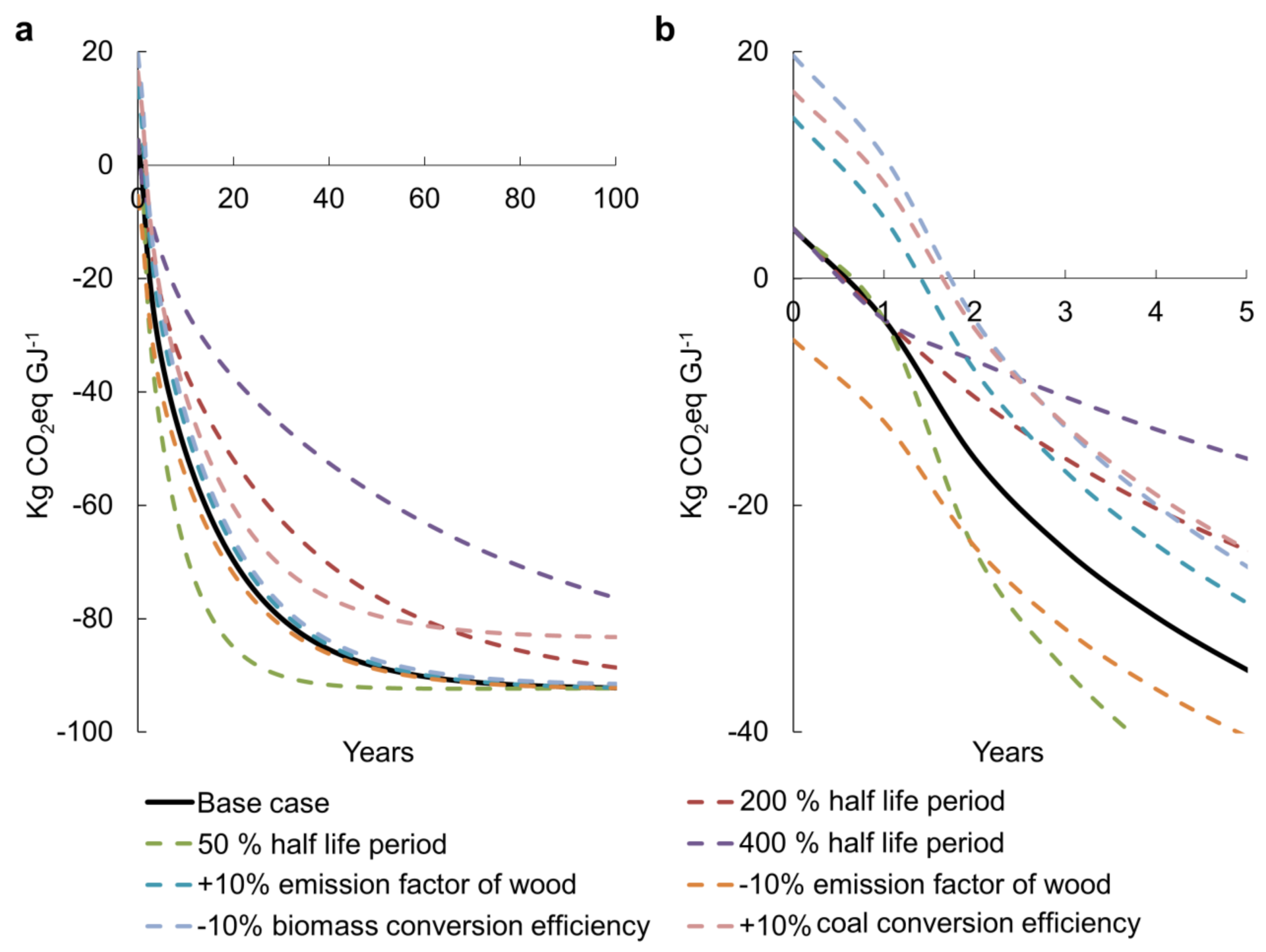
In this analysis, the carbon debt payback time is dependent on the decay rates of the different biomass resources supplied to the plant. The results are shown in Figure 5, which illustrates the difference in emissions between the two scenarios. It covers a 100-year period following the direct emissions in year 0.

We find that the payback of the carbon debt occurs almost immediately—within the first year. This means that after less than one year, the biomass-fired plant has a lower impact on global warming than the continued operation on coal would have had. The contribution to global warming mitigation increases further in the following years and throughout the modelling period. After 12 years, the cumulative GHG emissions in the biomass scenario will be half that of the reference scenario (

Table 4. Influence of the sensitivity analysis on estimated carbon debt and the period it takes to reach 50% reduction of GHG emissions in the biomass scenario compared to the reference scenario.

Sensitivity Parameter	Carbon Debt	50% Reduction Relative to Reference Scenario
	kg CO2eq GJ−1	Years
Base case	4.4	12
200% half-life period	4.4	22
50% half-life period	4.4	7
400% half-life period	4.4	43
10% increased emission factor of wood	14.2	14
10% decreased emission factor of wood	−5.4	10
10% decrease in biomass plant fuel efficiency	19.6	14
10% increase in coal plant fuel efficiency	16.5	14

). In other words, the global warming impact of the biomass scenario is reduced to half that of the reference scenario after 12 years.

Sensitivity

The test the sensitivity of the carbon debt payback time reported above key parameter values are changed returning alternative carbon debts (Table 4) and payback times (Figure 5). A slower decay rate of biomass left in the forest limits the benefits of the bioenergy scenario when compared to the reference scenario, at least in the short to medium term. Nevertheless, the biomass scenario will still achieve a rapid climate benefit compared to the reference scenario. The GHG emission factor for wood that is used in this analysis is generic. However, different tree species have different composition and ratios of carbon (C), hydrogen (H), and oxygen (O), and consequently different GHG emissions per unit of energy. If the emission factor of wood is increased by 10%, the carbon debt increases to 14.2 kg CO₂eq GJ⁻¹, however, the payback time is only increased by one year. By decreasing the emission factor of wood by 10%, the carbon debt becomes negative to −5.4 kg CO₂eq GJ⁻¹. This implies that the direct emissions from the biomass supply chain are lower than those from the coal supply chain, and that the biomass scenario will be immediately beneficial to climate change mitigation when compared to continued use of coal. Adjusting the power plant efficiency influences the carbon debt and payback time to a similar degree. Changing biomass decay rates (by changing the half-life period) does not affect the carbon debt, but only the payback time. Doubling the half-life period slows down the decay rate and increase the carbon debt payback time. The time it takes to achieve 50% reduction of GHG emissions from heat and electricity production is increased from 12 to 22 years (Table 4). With a 50% reduction in half-life periods a 50% reduction in GHG emissions is achieved after seven years. In the extreme case, with a four times increase of biomass half-life periods, the 50% reduction is achieved after 43 years.

4. Discussion

This study contributes to the body of literature on the climate mitigation potential of biomass as a replacement for coal in CHP production. Zetterberg & Chen [28] and Cintas et al. [29] analyzed scenarios for the use of forest residues to displace coal in CHP production in Scandinavian countries. Both of the studies reported carbon payback times of 0 years, corroborating the findings reported here. Colnes et al. [30] looked at the use of mixed resources (residues, thinning wood, round wood) from south-eastern USA to displace coal in CHP production and found a payback time of 35 years. The longer payback time reported for SE USA may be attributable to the fact that not only residue resources was included in the supply chain, but also dedicated harvests, which would not have been left to decay, but left to continued growth and carbon sequestration. Repo et al. [31] reported on electricity production in Finland using forest residues to displace coal with a carbon payback time of 0 years, while Cherubini et al. [32] for heat production in Norway using mixed wood resources to displace coal found a carbon payback time of 20 years. In correspondence with Colnes et al. [30], Cherubini et al. [32] reports longer payback times for a supply chain, including mixed wood resources. Also, Gustavsson et al. [26], Repo et al. [33], Sathre & Gustavsson [34], and Pingoud et al. [35] report carbon payback times close to 0 years in corroboration with this analysis suggesting almost immediate climate benefits from using thinning and residue wood instead of coal for heat and electricity production. A large number of studies have been carried out in other parts of the world on scenarios with comparable fuel source transformation reported here. Zanchi et al. [8], on forest residues to displace coal for electricity production in Austria, reported a payback time of 0 years. Lamers et al. [36], McKechnie et al. [37], and Ter-Mikaeliean et al. [38], studied forest residues to displace coal for electricity production in North America and reported carbon payback times between 0 and 30 years. Walker et al. [7], Daigneault et al. [39] also reported for North America carbon payback times between 0 and 75 years using mixed wood resources to displace coal in electricity production. The use of mixed wood resources seems to extend the payback period and also the production of electricity only significantly reduces the overall conversion efficiency. Gustavsson et al. [26], furthermore, coupled the emissions data with a Cumulative Radiative Forcing (CRF) model, which suggest a slower increase in climate benefits than a simple GHG emission balance portrayed in this study does. This is due to the immediate emission pulse and the long atmospheric residence time of a CO₂ molecule.

Studies comparing a biomass scenario to other fossil fuel scenarios, such as natural gas and oil [26,33,34,35], find considerable ‘carbon debts’ with longer payback times; however in the long term they all end up being more beneficial for the climate than the fossil alternative. In this case study, it is not relevant to look at alternative fuels or technologies, since its purpose is to evaluate the climatic benefits of a decision already made. Other alternatives may have been ruled out on the basis of economical, technological, political, or geographical limitations. These can however change in the future, which can alter the results. The reference scenario is key to these types of analyses and the reference scenario for the used biomass can also very quickly change due to market dynamics. If, as an example, the biomass used in the plant, instead of decaying on the forest floor, would have been used for other wood products, the resultant carbon payback time would change considerably. Changes in fuel conversion efficiency have proved to have a large influence on carbon debt and payback times; see e.g., Mitchell et al. [6]. Here, the biomass scenario exhibited slightly higher fuel efficiency than the reference scenario, 85.9% when compared to 84.2%. If the coal boiler had been replaced with a more modern coal boiler instead of a biomass boiler, the fuel efficiency of the reference scenario would likely have been higher than the biomass scenario. The sensitivity analysis demonstrates that fuel conversion efficiency has an influence on the carbon debt, but the payback time is not influenced much.

The major uncertainty in this study lies in the assumed biomass decay rates, since the wood is sourced from a great number of different locations in different climate regions. The local conditions, especially temperature and humidity, have a strong influence on decay rates. Over the long term (>100 years), slower decay rates are less influential. More complex modelling of decay rates, such as the Yasso07 model [40], suggest a quicker decline in decay rates than the exponential functions, which could influence climate benefits in the medium term (50 to 100 years).

5. Conclusions

In conclusion, this study shows that the use of biomass for energy is not carbon neutral in absolute terms. In the transition from fossil to biomass resources increased GHG emissions to the atmosphere can be expected. These are, however, quickly countered by fossil fuel savings and ecosystem responses. For the transition from coal to forest residues that would otherwise decay, for combined heat and power production in northern Europe, we find that a carbon debt of 4.4 kg CO₂eq GJ⁻¹ was paid back within one year. Furthermore, the results show that GHG emissions are reduced by 50% relative to continued coal combustion after about 12 years. While the results are sensitive to underlying assumptions, the sensitivity analysis showed little effect on carbon debts and payback times. For all scenario variations analyzed, the carbon debt is paid back within two years. The findings support the use of residue biomass for energy as an effective means for climate change mitigation, and for a transition away from fossil energy resources.