A Parameterization Approach for the Dielectric Response Model of Oil Paper Insulation Using FDS Measurements

Abstract

To facilitate better interpretation of dielectric response measurements—thereby directing numerical evidence for condition assessments of oil-paper-insulated equipment in high-voltage alternating current (HVAC) transmission systems—a novel approach is presented to estimate the parameters in the extended Debye model (EDM) using wideband frequency domain spectroscopy (FDS). A syncretic algorithm that integrates a genetic algorithm (GA) and the Levenberg-Marquardt (L-M) algorithm is introduced in the present study to parameterize EDM using the FDS measurements of a real-life 126 kV oil-impregnated paper (OIP) bushing under different controlled temperatures. As for the uncertainty of the EDM structure due to variable branch quantity, Akaike’s information criterion (AIC) is employed to determine the model orders. For verification, comparative analysis of FDS reconstruction and results of FDS transformation to polarization–depolarization current (PDC)/return voltage measurement (RVM) are presented. The comparison demonstrates good agreement between the measured and reconstructed spectroscopies of complex capacitance and tan δ over the full tested frequency band (10⁻⁴ Hz–10³ Hz) with goodness of fit over 0.99. Deviations between the tested and modelled PDC/RVM from FDS are then discussed. Compared with the previous studies to parameterize the model using time domain dielectric responses, the proposed method solves the problematic matching between EDM and FDS especially in a wide frequency band, and therefore assures a basis for quantitative insulation condition assessment of OIP-insulated apparatus in energy systems.

1. Introduction

The overall reliability of a power grid depends to a great extent on the sound operation of the grid-connected power apparatus. In the grid, power transformers, potential or current transformers, oil-filled power cables, and other oil-immersed high-voltage equipment substantially represent the critical assets thereof. The apparatus are subjected to intricate operational and loading conditions and thus encounter multifactor threats. For instance, a transformer may suffer from conditions like magnetizing inrush [1], overloading [2], and internal insulation faults like moistened or ageing insulation [3]. The composite media of oil-impregnated paper (OIP) constitutes the main internal insulation body of most equipment applied for high-voltage alternating current (HVAC) transmission. Faults in internal insulation are recognized as the main cause of failures in power equipment. For example, moisture in OIP insulation causes three dangerous effects: it decreases the dielectric withstanding strength, raises the emission of water vapor bubbles, and accelerates cellulose aging. Therefore, accurate tracking of the insulation state is necessary.

The three well-established methodologies of dielectric tests—return voltage measurement (RVM), polarization–depolarization current (PDC) measurement, and frequency dielectric spectroscopy (FDS)—are nonintrusive diagnostic measurements for condition assessment of the OIP insulation bodies in power appliances [4,5,6,7,8,9]. As a promising diagnostic tool, more recent interest has centered around FDS measurement [10,11], which is less noise sensitive during on-site practice, and more informative in terms of the response recorded in a wide frequency band typically between 1 mHz and 1 kHz under lower voltages (usually in a peak value of 200 V). The low-voltage excitation can avoid nonlinear effects that are subjected to strong applied electric fields [12]. On the other hand, a spectrum of readings helps to evaluate the moisture content efficiently. For example, two OIP-bushings might have the same power loss factor at a certain power frequency but may vary in their moisture content. This difference tends to be disregarded if only the measurement at a single frequency voltage is applied. By contrast, the response of OIP material under different conditions (e.g., moisture levels, ageing status) becomes distinguishable in both the lower and higher frequencies in FDS. Therefore, FDS development can facilitate more usable and reliable diagnosis of critical OIP equipment in power grids.

Better understanding and analysis of OIP status are only possible with potent interpretations of the dielectric response. In this case, a considerable body of literature is devoted to addressing mainly the application of FDS interpretation for evaluating OIP conditions regarding moisture content or ageing status. Such documented attempts can be roughly categorized as follows:

• Comparing dielectric responses with those recorded from standardized samples, also known as “fingerprints”, to present qualitative knowledge of the insulation state [13,14,15];
• Modeling the OIP system to match the responses to thereby understand the dependence of model parameters on insulation conditions [11,16,17,18,19,20];
• Deriving numerical characteristics from the traces and fitting with intuitional indicators, e.g., moisture percentage or the degree of polymerization (DP) to develop analytical formulas between them [10,21,22,23].

In the foregoing, equivalent circuit models are analogous to real physical systems of OIP, bridging the gap between the macroscopic response and microcosmic patterns of dielectric behaviors. Subsequent investigations on the parameter variations allow a transparent interpretation of the correlations between the response and insulation state. The interpretation of FDS measurements by a comparison of finite element values appears much easier than comparing the traces. It is not our aim here to develop any judgement or numerical evidence for the assessment. Our intention is only to provide, for those intending to use equivalent dielectric response models, an effective approach to estimating the model variables, as a basis for further quantitative analysis of OIP condition.

In particular, the involved considerations are model types, data sources, and algorithms. Except for mathematical approximation (e.g., the Cole–Cole model) [18,24], the majority physical models that take the form of equivalent circuits are based on the extended Debye model (EDM) [16,19]. Time domain responses (PDC, RVM) and frequency domain response (FDS) are the data sources. PDC and RVM have been most used for parameterizing the EDM, as with case studies in the literature [25,26,27,28,29,30,31,32,33]. Representative work can be found in the literature [19]; in particular, Tapan Saha et al. proposed a kind of stepwise approach to identify the EDM parameters from PDC. Jinding Cai et al. calculated the EDM parameters from RVM using an improved ant colony algorithm [26]. It is observed that in such practices, the parameterized equivalent circuits are proven to be satisfying, as the obtained circuits actualize an accurate reconstruction of recorded traces themselves, and also a reciprocal transformation between PDC and RVM [28,29]. However, in the above practical applications, a problem which arises most frequently when using PDC and RVM is that significant discrepancy exists between the measured and simulated FDS within higher frequencies (>1 Hz) [30,31,32,33]. The disagreement is considered a consequence of limitations in the sampling precision regarding high-frequency current when PDC starts, as well as the noise susceptibility of the time domain measurement. It is the inherent high-frequency inaccuracy of PDC and RVM data themselves that makes the formulated model demonstrate a poor match with higher frequency FDS.

To solve this problem, parameterizing EDM directly using FDS instead of PDC or RVM should therefore be carefully addressed, because a wideband FDS, as mentioned earlier [10,11], features better anti-interference and high-frequency precision, making it more suitable for parameter identification. Unfortunately, use of FDS in practice has rarely been reported. Tao Zhang et al. fitted a model using FDS recordings; however, the fitting effects are discussed only in lower frequencies (10⁻⁴ Hz–10 Hz) [34] and a tendency of larger deviation starting from 1 Hz is observed. With this in mind, the Authors have set out to solve the unsatisfying time domain parameterization by using FDS data in the present study.

To this end, in the present study, an effort has been made to identify EDM parameters based on the FDS measurements of a real-life oil-impregnated condenser bushing using a syncretic algorithm that integrates a genetic algorithm (GA) and a LevenbergMarquardt (LM) algorithm. A satisfactory parameterization effect regarding measured FDS is evidenced by the comparative analysis between the reconstructed FDS and the transformed PDC/RVM results. The paper is innovative in the following aspects: (a) different from all existing practices using PDC and RVM, a novel approach for EDM parameterization using FDS achieves perfect matching between EDM and FDS, especially in the full tested frequency band (10⁻⁴ Hz–10³ Hz); and (b) rather than using the default model orders of EDM conventionally, Akaike’s information criterion (AIC) is employed to indicate the optimal branch numbers in the EDM. The procedure to identify the circuit parameters will be detailed in the remainder of this paper.

2. Equivalent Model of OIP Insulation

The insulation structure is deemed as a continuous medium, comprising dipoles detached from each other. In the presence of an electric field, polarization arises inside dielectric materials when the dipoles align in the direction of the electric field [19]. Relaxation polarization is to be noted as it is significantly impacted by the material status. Therefore, the embedded indications in dielectric relaxation should be carefully evaluated.

A phenomenon worth stressing is the nonlinear dielectric effect (NDE), which describes the dielectric permittivity changes with higher orders of the electric field due to the application of a strong electric field. The fundamental hypothesis of the present study is that the dielectric response of OIP insulation holds linear under low excitation voltage of 200 V (peak value) in FDS tests. This assumption is fully justified because in the following experiments a genuine bushing was employed as the test samples, rather than using traditional pressboard. As the major OIP insulation part of the bushing is designed to withstand at least 126 kV, a 200 V test voltage raises a weak electric field which is low enough that NDE can be disregarded.

With this assumption, the dielectric response can be characterized by the extended Debye model, which is based on a linear circuit with R–C parallel structure (see Figure 1). The model arranges parallel combinations of multiple R–C series to represent dipole groups that have different relaxation time [29,35]. R_i and C_i (i = 1,…,n) indicate the polarization resistance and capacitance, respectively. R₀ and C₀ indicate the geometric resistance and capacitance, respectively.

With the circuit parameters known, the terminal admittance of the EDM can be written as

$$1/Z=j\omega C_0+1/R_0+{\displaystyle \sum _{i=1}^{n}1/\left(R_i+\frac{1}{j\omega C_i}\right)}.$$

(1)

The complex capacitance of dielectrics is defined as follows:

$$C^{*}=\frac{1}{j\omega Z}=C_0-\frac{1}{\omega R_0}j+{\displaystyle \sum _{i=1}^n\frac{C_i(1-j\omega R_i{C}_i)}{1+{(\omega R_i{C}_i)}^2}}.$$

(2)

The real and imaginary capacitance C′(ω), C″(ω) can therefore be given by

$$C^{\prime }(\omega )=\mathrm{Re}[\frac{1}{j\omega Z}]=C_0+{\displaystyle \sum _{i=1}^n\frac{C_i}{1+{(\omega R_i{C}_i)}^2}}$$

(3)

$$C^{″}(\omega )=-\mathrm{Im}[\frac{1}{j\omega Z}]=\frac{1}{\omega R_0}+{\displaystyle \sum _{i=1}^n\frac{\omega R_i{C}_i^2}{1+{(\omega R_i{C}_i)}^2}}.$$

(4)

The power loss factor is defined then as the ratio of C″(ω) and C′(ω):

$$\tan \delta =C^{″}(\omega )/C^{\prime }(\omega ).$$

(5)

Essentially, the EDM considers an insulation system as a “black box” [29]. The objectives of this paper are to determine a set of R_n and C_n so that the resulting terminal responses Equations (3)–(5) conform to the experimentally measured FDS data. Meanwhile, the obtained values of R_n and C_n should be physical. Please note that in our case, the two terms nonlinear “optimization” and “fitting” will not be strictly distinguished, and we shall use both terms hereafter, as they actually have the same essential meaning in this study.

3. Methodology of Model Parameterization

3.1. Problem Statement

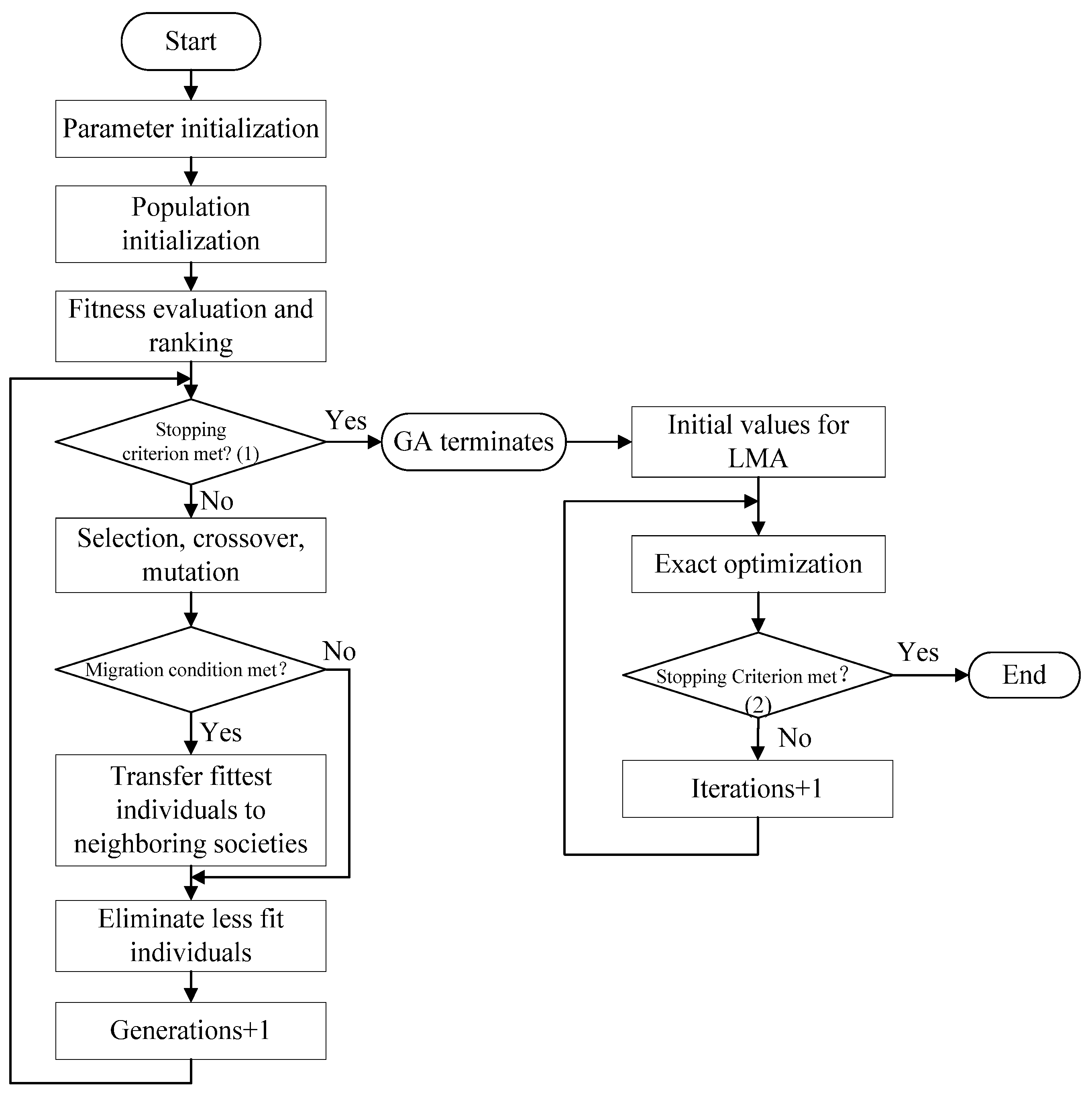
Fitting the model is a numerical trial and error experiment throughout the study. The following critical problems were found therein which need adaptations to any algorithms to achieve an exact and meaningful estimation of the model variables.

FDS results usually cover many magnitudes of the capacitance between the minimum and maximum frequencies (e.g., the measured imaginary capacitance of the OIP bushings ranges in the order of 10⁻¹¹–10⁻⁷). Common residue conditions worsen and only large-valued capacitance undergoes significant changes and achieves good approximation after several iterations. Therefore, the residue should be weighed. The capacitance and resistance in the model also extend over many magnitudes. Another similar maladaptation was encountered wherein small-valued capacitance goes through insignificant changes. Thus, the variables should be normalized.

Not least of these problems is that as the fitting effect can only be examined terminally, the identified capacitance and resistance inside the circuit may appear meaningless or unphysical, even if the overall FDS curves are precisely fitted. Well-recognized central ranges of R_i and C_i are 10⁹ Ω and 10⁻⁹ F, respectively, which have been validated by the work using the two time domain responses [19,25,26,27]. C₀ and R₀ should conform to nameplates or power frequency test results and the DC insulation resistance measurement. However, it is not recommended to apply any further constraints explicitly other than merely a fundamental nonnegativity restriction for each capacitor and resistor. Compulsory boundaries are very likely to significantly decrease the goodness of fit once unknown optimal solutions are excluded. As we shall see, fitting results that match the physical essence can be expected as long as the above two adaptations are correctly applied.

3.2. Algorithm

To address the multivariable and nonlinear optimization, common methods are gradient descent, the Gauss–Newton Algorithm (GNA), and the Levenberg–Marquardt Algorithm (LMA). The algorithms are highly dependent on proper initial values so as to secure rapid convergence [30,31]; however, while modeling engineering problems, correctly specifying or guessing any initial values is often not technically realizable, because practical parameters are always widely ranged. Early attempts of LMA by the authors have revealed that for less than three variables, the fitting can converge quickly with high accuracy; however, LMA tends to locate a local minimum if more than three variables are involved. Therefore, a single gradient-based algorithm seems to be powerless to solve the problem.

In this circumstance, a genetic algorithm (GA) is considered. GA is a sort of intelligent algorithm which has met with popularity in recent years and has fine universality and robustness. More importantly, GA features a strong global searching capability to avoid the local minimum point. However, it should also be noted that the algorithm lacks local searching capability and accuracy due to finite coding length.

With these facts in mind, GA and LMA were linked to solve the stated problem. Considering the respective advantages and weakness, GA was made responsible for an initial solution, from which LMA was then started to apply a secondary optimization. The combination makes use of GA’s strength in global search to locate a rough solution, providing reasonable initial values for LMA to launch a further exact search in the vicinity with the fast and accurate convergence properties of LMA. As they are individually very common and well-understood algorithms, the fundamentals of GA and LMA will not be discussed here. The flow chart is given in Figure 2 to illustrate the way in which GA and LMA were linked.

Stopping Criterion (1) of GA is when the maximum number of generations is reached, and Stopping Criterion (2) (Criterion (1) and (2) are denoted in Figure 2) is when the average fitness of the kth generation (fitness(x_k)) satisfies |fitness(x_k+1) − fitness(x_k)|_n ≤ ε.

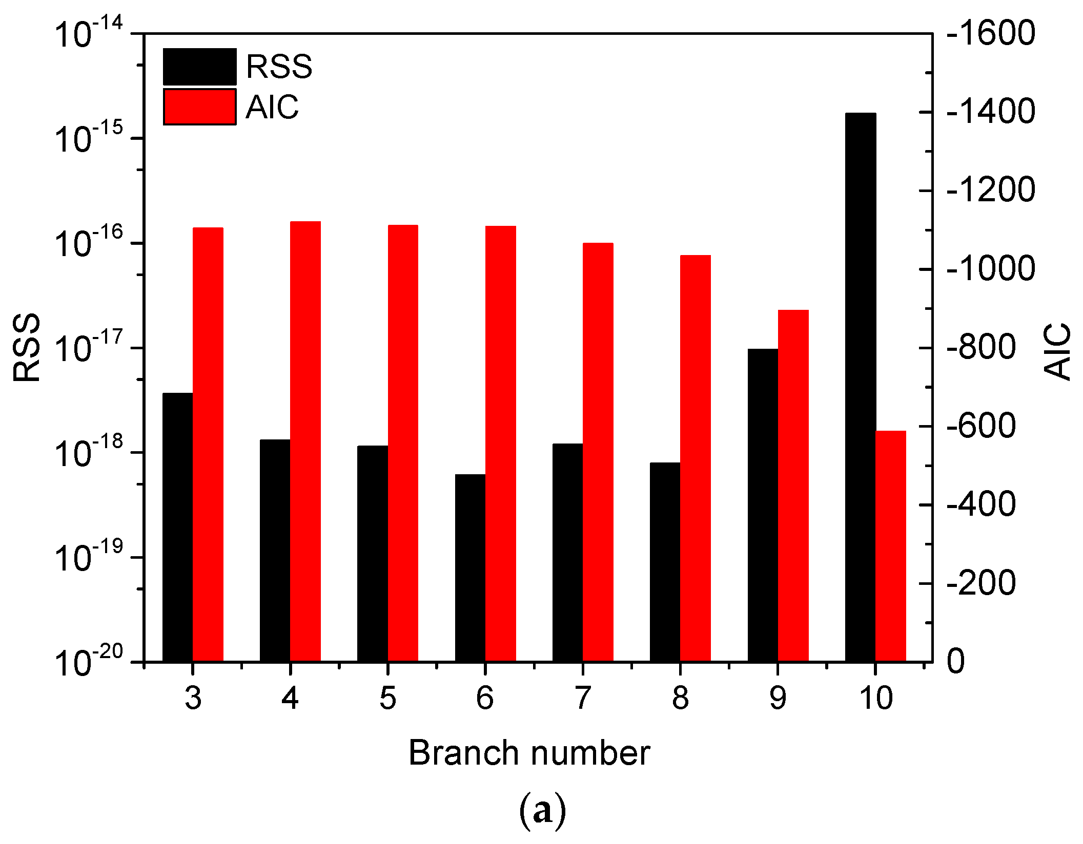
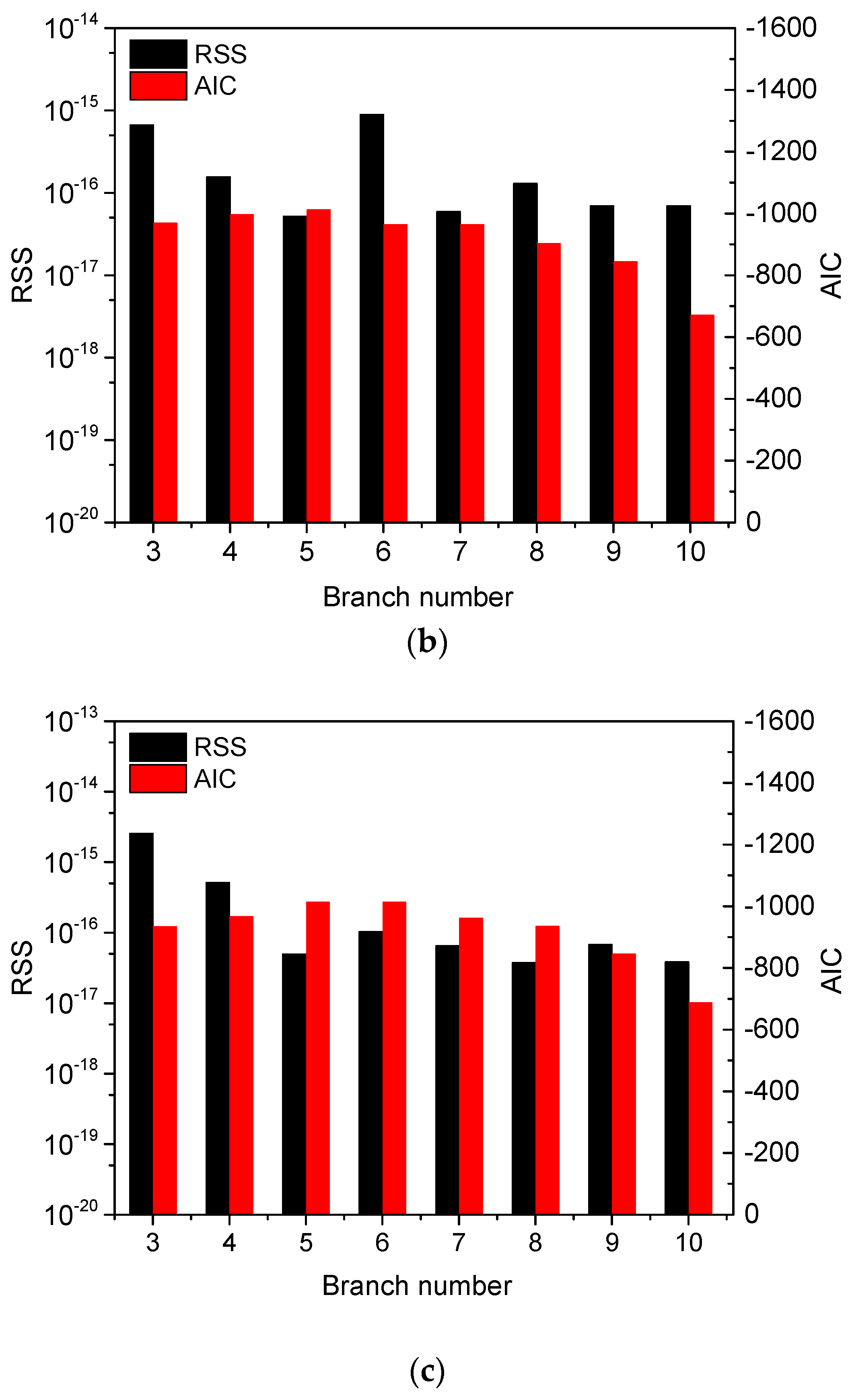
3.3. Akaike Information Criterion (AIC)

The EDM features a regular circuit structure, but with varying complexity, which can be determined only if the circuit branch quantity is specified. For instance, in most study cases, 4–6 branches are arranged in the model [17,19,26,27,34], which results in at least 10 fitted parameters.

In essence, paralleled branches are analogues to relaxation polarization with different relaxation time in dielectrics. Therefore, we can speculate that more branches can improve the goodness of fit naturally even if applied algorithms themselves have the same effectiveness, especially for impure dielectrics (e.g., aged insulation oil) in which the dielectric behavior is complicated by interfacial relaxation between ageing products. Theoretically, we can expect to use infinite R–C branches to simulate the dielectric response absolutely. However, to ensure usability of the model, parameter quantity should be controlled. The parallel branch number in most studies from the literature is six, and no further explanations are presented on this point. In the present study, the Akaike information criterion (AIC) [36,37,38] is introduced to quantify this uncertainty among the competing model complexities.

If residual sum of squares (RSS) is used as the fitting criterion, AIC can be calculated as

$$\mathrm{AIC}=m[\ln \left(\frac{RSS}{m}\right)]+2k$$

(6)

where m is the sample size; k is the number of fitted parameters; and RSS can be calculated as

$$RSS={\displaystyle \sum _{i=1}^m\left[{\left({C^{\prime }}_{\mathrm{mea}}(\omega )-{C^{\prime }}_{\mathrm{fit}}(\omega )\right)}^2+{\left({C^{″}}_{\mathrm{mea}}(\omega )-{C^{″}}_{\mathrm{fit}}(\omega )\right)}^2\right]}.$$

(7)

It should be noted that only two dozen points are usually available from any on-site FDS measurements, because of time-saving reasons at lower frequencies (<1 Hz). For small sample sizes (when m/k is less than 40 in the most complex model), a modified version of AIC (AICc) is recommended:

$$\mathrm{AICc}=\mathrm{AIC}+\frac{2k(k+1)}{m-k-1}.$$

(8)

It is clear that the term mln(RSS/m) quantifies the goodness of fit, for which smaller values of AIC can be obtained under better fitting. However, the second term 2k will increase if more parameters are involved in achieving this fitting. Therefore, the AIC index encourages better fitting and also tries to avoid overfitting. Thus, the optimal model should be that with smallest AIC value. The overall procedure is to apply the linked GA and LMA algorithm on each considered structure first, and then use AIC to determine the optimal parameterized model.

4. Case Study

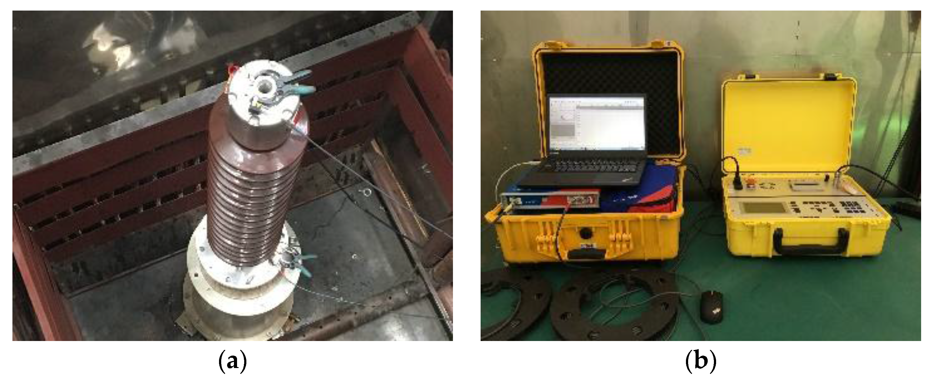
4.1. Dielectric Response Measurement

With the development of high-voltage direct current (HVDC) transmission, polymeric insulation material like polyethylene has been increasingly adopted in HVDC appliances [39], e.g., HVDC power cables. However, in the current stage, we limit the discussion here only to traditional OIP insulation, as OIP structures dominate insulation in most AC equipment at present. Therefore, as a typical case, an actual 126 kV OIP condenser transformer bushing was employed as a test sample to validate the proposed method. The three dielectric responses (PDC, RVM and FDS) of the OIP insulation body of the bushing were measured.

Figure 3a illustrates the structure of the OIP bushings. Typically, there are four main parts of a bushing: insulation, conductor, connection clamp, and accessories. It is in our interest to measure and model just the dielectric response of the major insulation—the condenser bodies. For a capacitance graded bushing, the condenser body (Figure 3b) is paper that is wound and impregnated with oil, and conducting layers are arranged within the body. By the recommended ungrounded specimen test (UST) method on the major insulation of bushings with test taps [40], the test voltage is directed and applied between the test tap and the conductor, which mainly reveals the dielectric response of the sandwiched body itself, while the impacts from the oil duct can be disregarded. Therefore, being a single insulation medium, the bushing insulation can be directly modelled and parameterized using the discussed method. For other cases, such as the insulation of a transformer, multiple insulation materials (oil, pressboard barriers, and pressboard spacers) are present in a certain geometric arrangement, which is always depicted by an X–Y model [6,18]. Measured dielectric response therein is the combined contribution from the composite insulation structures. Theoretically, the equivalent model in this case should be a network with each insulation part being a single EDM and connected as their physical arrangement [41]. This situation will not be discussed in the present paper.

A dielectric response analyzer (DIRANA) was used to measure the FDS and PDC of the bushing. RVM 5462 was used to measure the return voltage of the bushing. PDC and RVM, the two dielectric responses in the time domain, are not our focus in this paper, though we have tested all of the three dielectric responses for a comprehensive and comparative study crossing both time and frequency domains. The experimental setup is given in Figure 4 and the scheme of FDS instrumentation is illustrated in Figure 5.

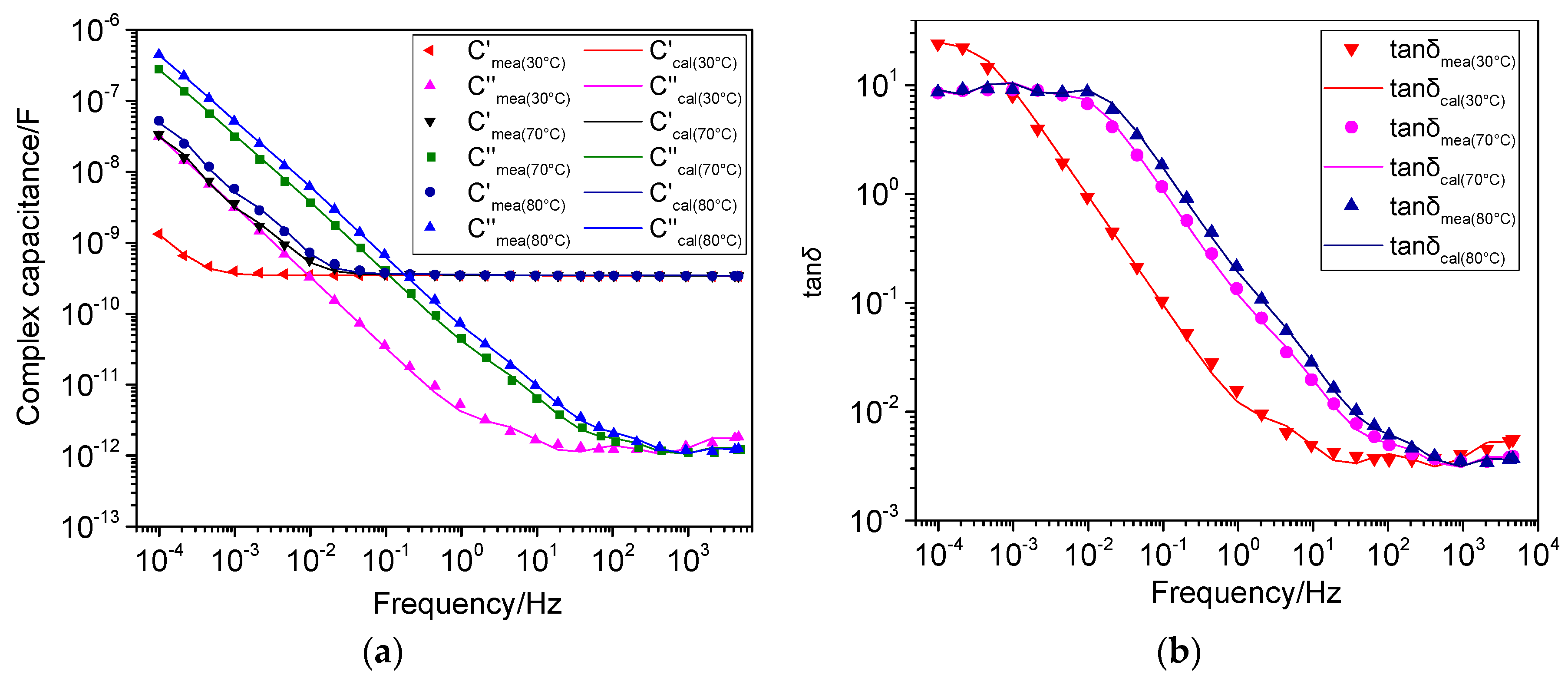
4.2. Parameter Identification Results

Parameter identification was applied to the three groups (under 30 °C, 70 °C, and 80 °C) of the tested FDS results. As the quantity of polarization branches is uncertain, branch numbers from 3 to 10 were attempted for each group. In each case, the residue RSS and AIC were calculated, as plotted in Figure 6. We clarify that only the polarization branch quantity is variable while the two geometry branches are constant. Therefore, for simplicity in the following, we use the term “branch number” and the symbol n to denote only the quantity of the paralleled R–C branches, rather than the total branch quantity that is defined conventionally from a perspective of circuit theory.

Figure 6a,b reveal that regarding the FDS results under 30 °C and 70 °C, the optimal branch numbers of EDM are 4 and 5, respectively, judging from the smallest AIC values. In Figure 6c, the AIC values of 5 and 6 appear the same. In this circumstance, the optimal branch number should be that with smaller RSS, namely 5. The three groups of AIC values also indicate a significant improvement of the goodness of fit only for n ≤ 5. When the branch number exceeds 5, this improvement can be weak or even uncertain. For n ≥ 10, the models are notably less competitive, because the increase in model complexity dominates the AIC rather than a decrease in fitting residues.

The fitted results are plotted against the measured FDS results (Figure 7) to show the effectiveness of the proposed parameterization method. Both the complex capacitance and tan δ are plotted under the three test temperatures, and the model parameters are listed in

Table 1. Goodness of fit of the FDS tested under the three temperatures: 30 °C, 70 °C, and 80 °C

Temperature (°C)	C′	C″	tan δ
30	0.9938	0.9985	0.9970
70	0.9992	0.9990	0.9929
80	0.9974	0.9996	0.9928

,

Table 2. The identified resistance and capacitance in extended Debye model (EDM) at 30 °C.

Branch No.	Ri (GΩ)	Ci (nF)	τi (s)
0	52.16955	0.32593	17.00362
1	850.57341	1.86212	1583.86976
2	12.60626	0.00324	0.04084
3	0.63505	0.00211	0.00134
4	0.01399	0.00334	4.67266 × 10−5

,

Table 3. The identified resistance and capacitance in EDM at 70 °C.

Branch No.	Ri (GΩ)	Ci (nF)	τi (s)
0	6.1842	0.32893	2.03417
1	23.89544	38.74998	925.94782
2	28.02376	1.82357	51.10329
3	5.36016	0.00994	0.05328
4	0.48943	0.00206	0.00101
5	0.01946	0.00232	4.51472 × 10−5

and

Table 4. The identified resistance and capacitance in EDM at 80 °C.

Branch No.	Ri (GΩ)	Ci (nF)	τi (s)
0	3.84327	0.33044	1.26997
1	15.23857	60.5265	922.33731
2	14.98666	3.24172	48.58256
3	4.63316	0.01374	0.06366
4	0.47013	0.00222	0.00104
5	0.02076	0.00219	4.54644 × 10−5

. The goodness of fit is given in Table 1.

The fitting index indicates that the determined parameters are accurate for reconstructing FDS results. C₀ and R₀ should be noted first as the two variables are essentially the geometry capacitance and resistance. The values are ratings which can be directly revealed by equipment nameplates or routing tests, such as the DC resistance test. To be physical, C₀ in EDM conforms to the rated capacitance of the tested bushing 330 pF. It is noteworthy that all the resistances and capacitances are obtained in the order of 10⁹ Ω and 10⁻⁹ F using the proposed algorithm, although no explicit constraints are applied to the variables. This range of polarization capacitance and resistance is widely accepted and in line with reported EDM parameters that are calculated from PDC or RVM [19,25,26,27].

As indicated by the low frequency dispersion (LFD) theory developed by Jonscher [42], in the LFD area where ωτ ≈ 1, as the temperature decreases, the average kinetic energy of charge carriers contained in the OIP system also declines; thus, the relaxation time rises and the LFD frequency descends. Therefore, the fitted insulation resistance R₀ is observed to decrease with the increase of temperature. This phenomenon can be formulated by the well-known Arrhenius relationship: μ = μ₀exp(−E_μ/kT), where μ is the mobility; E_μ is the activation energy; K is the Boltzmann constant; and T is the temperature. The time constant of each polarization branch that can be calculated by τ_i = R_i × C_i is also given and sorted in descending order. It is revealed that the largest time constant also decreases with the increase of temperature. The time constant can be understood as the time taken for dipole groups to establish the polarization, and the following equation helps to explain this phenomenon: τ = πexp(U/kT)/ω₀, where U is the barrier height in double-well potential; and ω₀ is the angular frequency of particle vibration [43]. The equation indicates that the time constant decreases exponentially as the temperature increases. Besides this, it is observed that as the temperature decreases, the capacitance in the maximum and submaximal time constant branches significantly decreases. This is because the mobility of charge and polar particles as well as the relaxation of dipole groups are retarded, which reduces the stored energy in the dipole, shown as a decline of capacitance in the polarization branches.

4.3. Polarization Current Modelled from FDS

Polarization and depolarization current (PDC) measurement as earlier mentioned is a nondestructive dielectric testing method to assess the insulation condition [3,4,28]. A DC voltage is applied to charge a test object for a period T_p. During the charging, the current flowing through the dielectric is recorded. The excitation voltage is then removed, and the test object is short-circuited to ground. The depolarization current that flows in the opposite direction due to the previously activated polarization process is recorded.

With the model parameters known, the polarization current can be transformed from the model. Under the circuit topology of EDM, the polarization current can be calculated as

$$i_p=\frac{U_0}{R_0}+{\displaystyle \sum _{i=1}^n[\frac{U_0}{R_i}\exp (-t/{\tau }_i)]}$$

(9)

where U₀ is the applied DC voltage for polarization, and τ_i presents the time constant of each polarization branch. Likewise, the depolarization current can be calculated as

$$i_d={\displaystyle \sum _{i=1}^n[A_i\exp (-t/{\tau }_i)]}$$

(10)

where the coefficient A_i is given by

$$A_i=\frac{U_0}{R_i}\left[1-\exp (-t_c/{\tau }_i)\right].$$

(11)

It is observed from Figure 8a that more significant deviation between the calculated and measured traces is located in the long time range than at the start of the polarization current. This is because the final portions of the polarization and depolarization currents are governed by R₀ and the largest time constant branch (denoted herein as B^1st), whereas the other exponential currents in Equations (9) and (10) attenuate and vanish well before that time (see the sum of multiple negative exponential terms in Equations (9) and (10)). Saha et al. explored the dependence of PDC and RVM on the R_i–C_i in each branch of EDM, and approached the same conclusion by comparing the changes of the two time domain responses, while varying the R_i–C_i in larger time constant branches [16]. Then, we rewrite C″(ω) Equation (4) in the form as Equation (12). This indicates that the spectrum of imaginary capacitance comprises n + 1 subspectra, among which the peak of the ith (i = 1,…,n) subspectrum appears at the angular frequency w = 1/τ_i. Therefore, R₀ and B^1st again dominate the low-frequency (LF) band of the imaginary capacitance. The LF C″(ω), in turn, is governing data to determine the value of R₀ and B^1st parameters if the FDS curves are precisely fitted.

However, LF C″(ω) or tan δ is susceptible to on-site interference and thus is of low accuracy under a frequency domain measurement. From a practical point of view, for any FDS testers, the lossy part (C″(ω) or tan δ) and lossless part (C′(ω)) are separated by tracing the angular lag between alternative voltages and response currents. Under low frequencies, the error of the measured angle is increased as the current becomes tiny. Experimental evidence is that discrepancy of recorded FDS from one tester is frequently encountered in lower frequencies (˂1 Hz) between repetitive FDS tests on the same sample and test conditions, while FDS in higher frequencies can mostly remain unchanged. Therefore, the determined R₀ and B^1st values from LF FDS are imprecise, which governs the difference between the measured and modelled PDC.

$$C^{″}(\omega )=\frac{1}{\omega R_0}+{\displaystyle \sum _{i=1}^n\frac{R_i{C}_i^2}{1/\omega +\omega {\tau }^2}}$$

(12)

4.4. RVM Modelled from FDS

Return voltage measurement is another dielectric response in the time domain. RVM is used to investigate slow polarization in the dielectric. This method is based on analysis of the curve of maximum recovery voltage versus charging time, the so-called polarization spectrum [3,32]. RVM includes the following steps. First, switch on S₁ and switch off S₂ (see Figure 9).

The voltage across C₀ is U₀ and the voltage across C_i after a charging period t_c is

$$U_{c_i}=U_0(1-e^{-t_c/R_i{C}_i}).$$

(13)

Then disconnect S₁ and switch on S₂. The dielectric discharge then. After a discharging period t_d, the voltage of C_i is

$$U_{ci}=U_0(1-e^{-t_c/R_i{C}_i})e^{-t_d/R_i{C}_i}.$$

(14)

Finally, disconnect S₂, and start the measurement of return voltage. The voltage across C₀ can be calculated as a superposition of contributions from C_i. In this case, the resulting U_ri from U_ci satisfies the following equation:

$$\frac{U_{ri}(s)}{U_{Ci}(s)}=\frac{s^n{N}_{n,i}+s^{n-1}{N}_{n-1,i}+\dots +N_0}{s^{n+1}{D}_{n+1}+s^n{D}_n+s^{n-1}{D}_{n-1}+\dots +D_0}$$

(15)

where N and D are coefficients that correlate with each resistor and capacitor in the circuit. The U_ci in the time domain can be obtained by applying inverse Laplace transform regarding U_ci(s). The total U_r can be calculated as

$$\begin{array}{l}{U}_{\mathrm{m}}(t_p)=U_0{A}_{\max 1}(t_p)(1-\exp (-t_c/{\tau }_1))\exp (-t_c/2{\tau }_1)\\ +\dots +U_0{A}_{\mathrm{maxn}}(t_p)(1-\exp (-t_c/{\tau }_n))\exp (-t_c/2{\tau }_n)\end{array}$$

(16)

where

$$\begin{array}{l}{A}_{\mathrm{maxi}}(t_p)=A_{i,1}\exp (p_1{t}_p)+\dots +A_{i,n+1}\exp (p_{n+1}{t}_p)\\ A_{i,j}=\frac{k_i}{p_j}\frac{{\displaystyle {\prod }_l(p_j-z_{i,l})}}{{\displaystyle {\prod }_{k\ne j}(p_j-p_k)}}\\ j,k=1,2,\dots ,n+1\\ i,l=1,2,\dots ,n\\ k_i=\frac{N_{n,i}}{D_{N+1}}\end{array}$$

(17)

where p_i is the pole of the transfer function; z_i,l is the zero of the transfer function under C_i; and P_i is the time when the return voltage reaches its peak.

If the charging time is varied, then the recorded peaks of return voltage versus charging time can be obtained; these are the RVM spectra. In RVM tests, the charging voltage was set to 500 V and a set of nine different charging time sequences ranging from 0.02 s to 10 s was applied. The ratio of charge/discharge time was set as 2. The measured and calculated peaks of recovery voltage are plotted against charge time in Figure 10.

Figure 10 demonstrates that the modeled RVM spectra from parameterized EDM approximate the measured results in the short time range of charging (t_c ˂ 1 s). However, more significant discrepancy is observed in the long time range. The modelling error in low frequencies from FDS data governs these differences.

In the same work we have referenced [16], it is also illustrated that the variations of R_i–C_i in larger time constants and R₀ will not prominently affect the front portion of the RVM spectra, but a noticeable shift in the subsidiary peak of RVM spectra is observed with the change of R₀ and large time constants R_i–C_i. Besides this, another influential factor is the nonlinear characteristic in the dielectric response because 500 V DC is applied in RVM, which is higher than the 200 V (peak value) in the FDS tests.

5. Conclusions

The extended Debye model was employed in this paper to characterize the dielectric response of insulation bodies in OIP bushings. In order to obtain the parameters in the equivalent circuit of EDM, a syncretic algorithm that integrates a genetic algorithm (GA) and the Levenberg–Marquardt (L-M) algorithm was applied to solve the optimization using the recorded FDS of an OIP bushing at 30 °C, 70 °C, and 80 °C. We adopted Akaike’s information criterion (AIC) to determine the branch numbers, or model orders. To balance the model approximation and complexity by choosing the smallest AIC values, we have optimal branch quantities of 4, 5, and 5, respectively, under the three controlled temperatures.

Once the model structure was determined with the model parameters known, all the dielectric responses, both in time and frequency domains, were simulated. The parameterization effectiveness was then examined by reconstructing FDS and FDS transformation to PDC/RVM. Comparative analysis of the measured and simulated results were presented. A good agreement with FDS measurements was observed across a wide band (10⁻⁴ Hz–10³ Hz) where FDS is recorded, with the goodness of fit of the real/imaginary capacitance and power loss factor all over 0.99. Simulated PDC approximates measured results at the start while deviation was found in the current tail (t > 1000 s). A similar discrepancy was observed in RVM tests. The difference is considered to be due to the noise susceptibility of FDS measurement, especially at low frequency.

The present paper is dedicated to seeking and justifying an effective method to calculate EDM branch parameters. On this basis, further research is intended to carefully investigate the manner in which oil and paper conditions affect the parameters, so as to achieve a clear interpretation of the FDS diagnosis.

References

1. Lee, B.; Park, J.W.; Crossley, P.A.; Kang, Y.C. Induced Voltages Ratio-based Algorithm for Fault Detection and Faulted Phase and Winding Identification of a Three-winding Power Transformer. Energies 2014, 7, 6031–6049. [Google Scholar] [CrossRef]
2. Wang, C.; Wu, J.; Wang, J.; Zhao, W. Reliability Analysis and Overload Capability Assessment of Oil-immersed Power Transformers. Energies 2016, 9, 43. [Google Scholar] [CrossRef]
3. Godina, R.; Rodrigues, E.M.G.; Matias, J.C.O.; Catalão, J.P.S. Effect of Loads and Other Key Factors on Oil-transformer Ageing: Sustainability Benefits and Challenges. Energies 2015, 8, 12147–12186. [Google Scholar] [CrossRef]
4. Martin, D.; Saha, T. A Review of the Techniques Used by Utilities to Measure the Water Content of Transformer Insulation Paper. IEEE Electr. Insul. Mag. 2017, 33, 8–16. [Google Scholar] [CrossRef]
5. Fofana, I.; Hadjadj, Y. Electrical-Based Diagnostic Techniques for Assessing Insulation Condition in Aged Transformers. Energies 2016, 9, 679. [Google Scholar] [CrossRef]
6. Gubanski, S.M.; Boss, P.; Csepes, G.; Der, H.V.; Filippini, J.; Guuinic, P.; Gäfvert, U.; Karius, V.; Lapworth, J.; Urbani, G. Dielectric Response Methods for Diagnostics of Power Transformers. IEEE Electr. Insul. Mag. 2003, 19, 12–18. [Google Scholar] [CrossRef]
7. Koch, M.; Prevost, T. Analysis of Dielectric Response Measurements for Condition Assessment of Oil-Paper Transformer Insulation. IEEE Trans. Dielectr. Electr. Insul. 2012, 19, 1908–1915. [Google Scholar] [CrossRef]
8. Setayeshmehr, A.; Fofana, I.; Eichler, C.; Akbari, A.; Borsi, H.; Gockenbach, E. Dielectric Spectroscopic Measurements on Transformer Oil-paper Insulation under Controlled Laboratory Conditions. IEEE Trans. Dielectr. Electr. Insul. 2008, 15, 1100–1111. [Google Scholar] [CrossRef]
9. Tenbohlen, S.; Coenen, S.; Djamali, M.; Müller, A.; Samimi, M.H.; Siegel, M. Diagnostic Measurements for Power Transformers. Energies 2016, 9, 347. [Google Scholar] [CrossRef]
10. Xia, G.; Wu, G.; Gao, B.; Yin, H.; Yang, F. A New Method for Evaluating Moisture Content and Aging Degree of Transformer Oil-Paper Insulation Based on Frequency Domain Spectroscopy. Energies 2017, 10, 1195. [Google Scholar] [CrossRef]
11. Hadjadj, Y.; Meghnefi, F.; Fofana, I.; Ezzaidi, H. On the Feasibility of Using Poles Computed from Frequency Domain Spectroscopy to Assess Oil Impregnated Paper Insulation Conditions. Energies 2013, 6, 2204–2220. [Google Scholar] [CrossRef]
12. Smith, D.J.; McMeekin, S.G.; Stewart, B.G.; Wallace, P.A. A Dielectric Frequency Response Model to Evaluate the Moisture Content within an Oil Impregnated Paper Condenser Bushing. IET Sci. Meas. Technol. 2013, 7, 223–231. [Google Scholar] [CrossRef]
13. Raetzke, S.; Koch, M.; Anglhuber, M. Modern Insulation Condition Assessment for Instrument Transformers. In Proceedings of the 2012 IEEE International Conference on Condition Monitoring and Diagnosis, Bali, Indonesia, 23–27 September 2012. [Google Scholar]
14. Koch, M.; Raetzke, S.; Krueger, M. Moisture Diagnostics of Power Transformers by a Fast and Reliable Dielectric Response Method. In Proceedings of the Conference Record of the 2010 IEEE International Symposium on Electrical Insulation, San Diego, CA, USA, 6–9 June 2010. [Google Scholar]
15. Gao, J.; Yang, L.; Wang, Y.; Liu, X.; Lv, Y.; Zheng, H. Condition Diagnosis of Transformer Oil-paper Insulation Using Dielectric Response Fingerprint Characteristics. IEEE Trans. Dielectr. Electr. Insul. 2016, 23, 1207–1218. [Google Scholar] [CrossRef]
16. Zhang, Y.; Liu, J.; Zheng, H.; Wei, H.; Liao, R. Study on Quantitative Correlations Between the Ageing Condition of Transformer Cellulose Insulation and the Large Time Constant Obtained from the Extended Debye Model. Energies 2017, 10, 1842. [Google Scholar] [CrossRef]
17. Fofana, I.; Hemmatjou, H.; Meghnefi, F.; Farzaneh, M.; Setayeshmehr, A.; Borsi, H.; Gockenbach, E. On the Frequency Domain Dielectric Response of Oil-paper Insulation at Low Temperatures. IEEE Trans. Dielectr. Electr. Insul. 2010, 17, 799–807. [Google Scholar] [CrossRef]
18. Gao, J.; Yang, L.; Wang, Y.; Qi, C.; Hao, J.; Liu, J. Quantitative Evaluation of Ageing Condition of Oil-paper Insulation Using Frequency Domain Characteristic Extracted from Modified Cole-Cole Model. IEEE Trans. Dielectr. Electr. Insul. 2015, 22, 2694–2702. [Google Scholar] [CrossRef]
19. Saha, T.K.; Purkait, P.; Muller, F. Deriving an Equivalent Circuit of Transformers Insulation for Understanding the Dielectric Response Measurements. IEEE Trans. Power Deliv. 2005, 20, 149–157. [Google Scholar] [CrossRef]
20. Verma, H.C.; Verma, H.C.; Baral, A.; Pradhan, A.K.; Chakravorti, S. Condition Assessment of Various Regions within Non-uniformly Aged Cellulosic Insulation of Power Transformer Using Modified Debye Model. IET Sci. Meas. Technol. 2017, 11, 939–947. [Google Scholar] [CrossRef]
21. Baral, A.; Chakravorti, S. Condition Assessment of Cellulosic Part in Power Transformer Insulation Using Transfer Function Zero of Modified Debye Model. IEEE Trans. Dielectr. Electr. Insul. 2014, 21, 2028–2036. [Google Scholar] [CrossRef]
22. Liao, R.; Liu, J.; Yang, L.; Gao, J.; Zhang, Y.; Lv, Y.; Zheng, H. Understanding and Analysis on Frequency Dielectric Parameter for Quantitative Diagnosis of Moisture Content in Paper-oil Insulation System. IET Electr. Power Appl. 2015, 9, 213–222. [Google Scholar] [CrossRef]
23. Liao, R.; Liu, J.; Yang, L.; Wang, K.; Hao, J.; Ma, Z.; Gao, J.; Lv, Y. Quantitative Analysis of Insulation Condition of Oil-paper Insulation Based on Frequency Domain Spectroscopy. IEEE Trans. Dielectr. Electr. Insul. 2015, 22, 322–334. [Google Scholar] [CrossRef]
24. Giselbrecht, D.; Leibfried, T. Modelling of Oil-Paper Insulation Layers in the Frequency Domain with Cole-Cole Functions. In Proceedings of the Conference Record of the 2006 IEEE International Symposium on Electrical Insulation, Toronto, ON, Canada, 11–14 June 2006. [Google Scholar]
25. Zheng, J.; Jiang, X.; Cai, J. Parameter Identification for Equivalent Circuit of Transformer Oil-paper Insulation and Effect of Insulation Condition on Parameters. Electr. Power Autom. Equip. 2015, 35, 168–172. [Google Scholar] [CrossRef]
26. Jiang, X.B.; Huang, Y.J.; Lai, X.S. Improved Ant Colony Algorithm and its Application in Parameter Identification for Dielectric Response Equivalent Circuit of Transformer. High Volt. Eng. 2011, 37, 1982–1988. [Google Scholar] [CrossRef]
27. He, D.; Cai, J. Method for Parameter Identification of Equivalent Circuit of Oil-paper Insulation and Its Research. High Volt. Eng. 2017, 43, 1988–1994. [Google Scholar] [CrossRef]
28. Liu, J. Investigation of Time-Frequency Hybrid Insulation Diagnosis Method Based on PDC Analysis. Ph.D. Thesis, Harbin University of Science and Technology, Harbin, China, 2014. [Google Scholar]
29. Sarkar, S.; Sharma, T.; Baral, A.; Chatterjee, B.; Dey, D.; Chakravorti, S. An Expert System Approach for Transformer Insulation Diagnosis Combining Conventional Diagnostic Tests and PDC, RVM Data. IEEE Trans. Dielectr. Electr. Insul. 2014, 21, 882–891. [Google Scholar] [CrossRef]
30. Kumar, A.; Mahajan, S.M. Correlation between Time and Frequency Domain Measurements for the Insulation Diagnosis of Current Transformers. In Proceedings of the North American Power Symposium, Arlington, TX, USA, 26–28 September 2010. [Google Scholar]
31. Kumar, A.; Mahajan, S.M. Time Domain Spectroscopy Measurements for the Insulation Diagnosis of a Current Transformer. IEEE Trans. Dielectr. Electr. Insul. 2011, 18, 1803–1811. [Google Scholar] [CrossRef]
32. Xu, S.; Middleton, R.; Fetherston, F.; Pantalone, D. A Comparison of Return Voltage Measurement and Frequency Domain Spectroscopy Test on High Voltage Insulation. In Proceedings of the 7th International Conference on Properties and Applications of Dielectric Materials, Nagoya, Japan, 1–5 June 2003. [Google Scholar]
33. Liu, J.; Zhang, D.; Wei, X.; Karimi, H.R. Transformation Algorithm of Dielectric Response in Time-frequency Domain. Math. Probl. Eng. 2014. [Google Scholar] [CrossRef]
34. Zhang, T.; Li, X.; Lv, H.; Tan, X. Parameter Identification and Calculation of Return Voltage Curve Based on FDS Data. IEEE Trans. Appl. Superconduct. 2014. [Google Scholar] [CrossRef]
35. Jota, P.R.S.; Islam, S.M.; Jota, F.G. Modeling the Polarization Spectrum in Composite Oil/paper Insulation Systems. IEEE Trans. Dielectr. Electr. Insul. 1999, 6, 145–151. [Google Scholar] [CrossRef]
36. Bozdogan, H. Model Selection and Akaike Information Criterion (AIC)—The General-Theory and its Analytical Extensions. Psychometrika 1987, 52, 345–370. [Google Scholar] [CrossRef]
37. Bozdogan, H. Akaike’s Information Criterion and Recent Developments in Information Complexity. J. Math. Psychol. 2000, 44, 62–91. [Google Scholar] [CrossRef] [PubMed]
38. Symonds, M.R.E.; Moussalli, A. A Brief Guide to Model Selection, Multimodel Inference and Model Averaging in Behavioural Ecology Using Akaike’s Information Criterion. Behav. Ecol. Sociobiol. 2011, 65, 13–21. [Google Scholar] [CrossRef]
39. Pourrahimi, A.M.; Olsson, R.T.; Hedenqvist, M.S. The Role of Interfaces in Polyethylene/metal-oxide Nanocomposites for Ultrahigh-voltage Insulating Materials. Adv. Mater. 2018. [Google Scholar] [CrossRef] [PubMed]
40. IEEE. Standard General Requirements and Test Procedure for Power Apparatus Bushings; IEEE Std C57.19.00-2004 (Revision of IEEE Std C57.19.00-1991); IEEE: Piscataway Township, NJ, USA, 2005; pp. 1–17. [Google Scholar]
41. Pradhan, A.K.; Chatterjee, B.; Chakravorti, S. Estimation of Dielectric Dissipation Factor of Cellulosic Parts in Oil-paper Insulation by Frequency Domain Spectroscopy. IEEE Trans. Dielectr. Electr. Insul. 2016, 23, 2720–2729. [Google Scholar] [CrossRef]
42. Jonscher, A.K. Dielectric Relaxation in Solids; Chelsea Dielectric Press: London, UK, 1983. [Google Scholar]
43. Zhongnan, X. Study on Simulation and Experiment of Polarization and Depolarization Current for Oil-Paper Insulation Ageing. Master’s Thesis, Chongqing University, Chongqing, China, 2011. [Google Scholar]
Figure 1. The structure of the extended Debye model.
Energies 11 00622 g001
Figure 2. The flow chart of the combination of the genetic algorithm (GA) and the Levenberg–Marquardt Algorithm (LMA).
Energies 11 00622 g002
Figure 3. Illustration of an oil-impregnated paper (OIP) bushing (not to scale): (a) overall structure; (b) the condenser body.
Energies 11 00622 g003
Figure 4. (a) OIP condenser bushing placed in an oast house for tests; (b) dielectric response analyzer and recovery voltage meter.
Energies 11 00622 g004
Figure 5. Scheme of frequency domain spectroscopy (FDS) instrumentation on the bushing.
Energies 11 00622 g005
Figure 6. The residual sum of squares (RSS) and Akaike information criterion (AIC) values of the parametrization results with different branch numbers under the three controlled temperatures: (a) 30 °C; (b) 70 °C; (c) 80 °C.
Energies 11 00622 g006aEnergies 11 00622 g006b
Figure 7. The reconstructed FDS from the parametrized model and the measured FDS: (a) complex capacitance; (b) tanδ.
Energies 11 00622 g007
Figure 8. (a) Polarization current; (b) depolarization currents modelled from the parameterized EDM using FDS measurements.
Energies 11 00622 g008
Figure 9. The scheme of return voltage measurement (RVM) test.
Energies 11 00622 g009
Figure 10. Measured vs. reconstructed RVM spectra modelled from the parameterized EDM using FDS measurements.
Energies 11 00622 g010