Accounting for Energy Cost When Designing Energy-Efficient Wireless Access Networks

Abstract

Because of the increase of the data traffic demand, wireless access networks, through which users access telecommunication services, have expanded, in terms of size and of capability and, consequently, in terms of power consumption. Therefore, costs to buy the necessary power for the supply of base stations of those networks is becoming very high, impacting the communication cost. In this study, strategies to reduce the amount of money spent for the purchase of the energy consumed by the base stations are proposed for a network powered by solar panels, energy batteries and the power grid. First, the variability of the energy prices is exploited. It provides a cost reduction of up to 30%, when energy is bought in advance. If a part of the base stations is deactivated when the energy price is higher than a given threshold, a compromise between the energy cost and the user coverage drop is needed. In the simulated scenario, the necessary energy cost can be reduced by more than 40%, preserving the user coverage by greater than 94%. Second, the network is introduced to the energy market: it buys and sells energy from/to the traditional power grid. Finally, costs are reduced by the reduction of power consumption of the network, achieved by using microcell base stations. In the considered scenario, up to a 31% cost reduction is obtained, without the deterioration of the quality of service, but a huge Capex expenditure is required.

1. Introduction

During the last few years, the number of mobile devices, as well as the capacity required by applications running on them, has grown. Consequently, the data traffic has increased and will increase. The work in [1] forecasts that mobile data traffic will grow at a compound annual growth rate of 47% until 2021. Because of this trend, the communication network has expanded, as well, in terms of size and of provided capacity to guarantee the required quality of service. This has an impact on the network energy consumption. In 2008, wired and wireless communication networks were already responsible for 15% of the electricity consumption of ICT (Information and Communication Technology). Within communication networks, wireless access networks, through which end users access telecommunication services, are large power consumers. Up to 80% of the energy consumption in 3G and LTE (Long-Term Evolution) is caused by the base stations that compose those networks.

In this way, access networks contribute to the general increase of the power consumption of these years, caused by ICT [2]. However, most of the energy we use today comes from fossil fuels, as mentioned in [3]. Fossil fuels are not renewable. This means that in the future, we will have a possible depletion if we continue to use them as we do today. Furthermore, it is supposed that political instability in oil-producing countries can result in severe oil price shocks, with devastating effects for economies based on this. Today, we have already noticed a significant increase in energy cost.

Besides the possible future depletion and the increase of energy cost, burning fossil fuels also causes the emission of carbon dioxide, which directly contributes to climate change.

For the reasons mentioned above, in the literature, much effort has been put toward designing energy-efficient wireless access networks. In [4], a capacity-based wireless access network is analyzed: the network responds to the instantaneous bit rate requested by the active users, switching part of the active base stations to sleep mode. Furthermore, it is demonstrated that the presence of different types of base stations results in a power consumption reduction. In this case, the wireless access network is composed by both macrocell base stations and microcell base stations, which provide a coverage area and a power consumption smaller than the macrocell base stations, as described in [5]. Moreover, wireless access networks powered with renewable energy sources (i.e., with solar and wind energy) are proposed. The work in [6] considers a cellular network where a part of the base stations is supplied by renewable energy only, while others are only connected to the traditional power grid. A base station sleep policy is used in order to save energy, based on energy and traffic predictions. A simpler heuristic algorithm is also proposed. It defines the number of active renewable powered base stations, based on traffic demand. The deactivation of grid-powered base stations is left to a dynamic programming algorithm. The work in [7] proposes a cloud based on heterogeneous cellular networks with hybrid energy sources. An optimization problem is formulated to reduce the energy consumption and to balance the load among base stations. The work in [8] investigates a portion of a mobile access network where base stations, equipped with Photovoltaic (PV) panels and energy storage, can be powered either by solar energy or by the power grid. A base station switching on/off policy operates in a centralized way to reduce energy consumption. It makes the decision depending on the actual traffic load, guaranteeing a minimum capacity for satisfying the current user demand, considering real location data about traffic and solar irradiation. Optimal system dimensioning is also investigated. In [9], the authors study the problem of energy efficiency in cellular heterogeneous networks using radio resource and power management combined with a BS switching on/off approach. The developed framework is employed to provide an efficient use of the radio resources and a minimization of the energy consumption. Two methods are proposed, providing an optimal and near optimal solution to the problem. The work in [10] investigates the energy and the network performance of a wireless access network powered by the traditional electricity grid, a PV panel system and an energy storage system. An energy-aware management system is proposed. It consists of the management of the energy provisioning and storage system and the application of energy-reducing strategies, which aim to minimize the amount of energy bought from the traditional power grid.

In these studies, and often in the literature, the aspect of the necessary energy cost to supply the base stations of the wireless access network is neglected. Nevertheless, studies that take care of minimizing the necessary energy cost are available in the literature. The work in [11] proposes a generic mixed-integer linear programming model to obtain job scheduling on a single machine to achieve the objective mentioned above, with the activation or deactivation of it according to the energy price.

Energy prices are becoming more volatile, since they depend on real-time demand and generation. In fact, they are used in the DR (Demand and Response) scheme. This is a program of the DSM (Demand Side Management) of the electricity system, which consists of mechanisms that aim at modifying the consumer’s demand profile, in time and/or shape, to make it match the supply to avoid overloads of the grid or the wasting of energy [12]. In this way, peaks higher than the normal demand are reduced. The presence of peaks in the power demand compromises the usage of renewable energy resources, since they are not reliable for the production of those amounts of energy. The DR acts against them with the introduction of the power utility’s incentive (incentive-based approach) or with the variation of electricity price (price-based approach). In particular, during peak hours, customers are induced to avoid consuming energy because of higher energy prices or penalties. In this way, they are encouraged to shift their demand during off-peak hours because of lower energy prices or a discount on their bill.

Concerning the price-based approach, different policies exist, as explained in [13]. For example, in the real-time pricing mechanism, prices vary over quite short periods (e.g., 1 h or 15 min), and they are released shortly in advance (the day before). In time-of-use pricing, they differ by time periods, but they remain constant within one period; in critical peak pricing, prices are increased in the case of critical overloads.

In this paper, the attention is focused on the cost for the purchase of the energy needed for the supply of the base stations of an energy-efficient wireless access network. To the best of the authors’ knowledge, this has never been investigated in this kind of network before. Our study builds on prior studies of the green-networking field, specifically the [14] one. The work in [14] introduces a capacity-based wireless access network, powered by a PV panel system, energy batteries and the power grid. It proposes an energy-management system. It consists of the management of the energy provisioning and storage system. Energy-saving strategies are also applied, which aim to reduce the amount of energy that should be bought from the power grid in case a renewable energy shortage occurs.

In this study, strategies and algorithms, which aim at the minimization of the necessary energy cost in the described scenario, are designed and discussed. A strategy achieves the aforementioned goal towards the decrease of the power consumption. Others exploit the dynamism of the energy price. Finally, the reduction of the energy cost is obtained with the introduction of the network in the energy market.

The main contributions offered in this paper are the following:

• it introduces and discusses new algorithms for the energy cost minimization;
• it shows that the decrease of the power consumption reduces the necessary energy cost, since the amount of the energy bought is smaller. It is also shown that the reduction of the network power consumption can be obtained with the usage of a network composed of microcell base stations only;
• it proves that the exploitation of the prosumer status of the considered network can reduce the necessary energy cost;
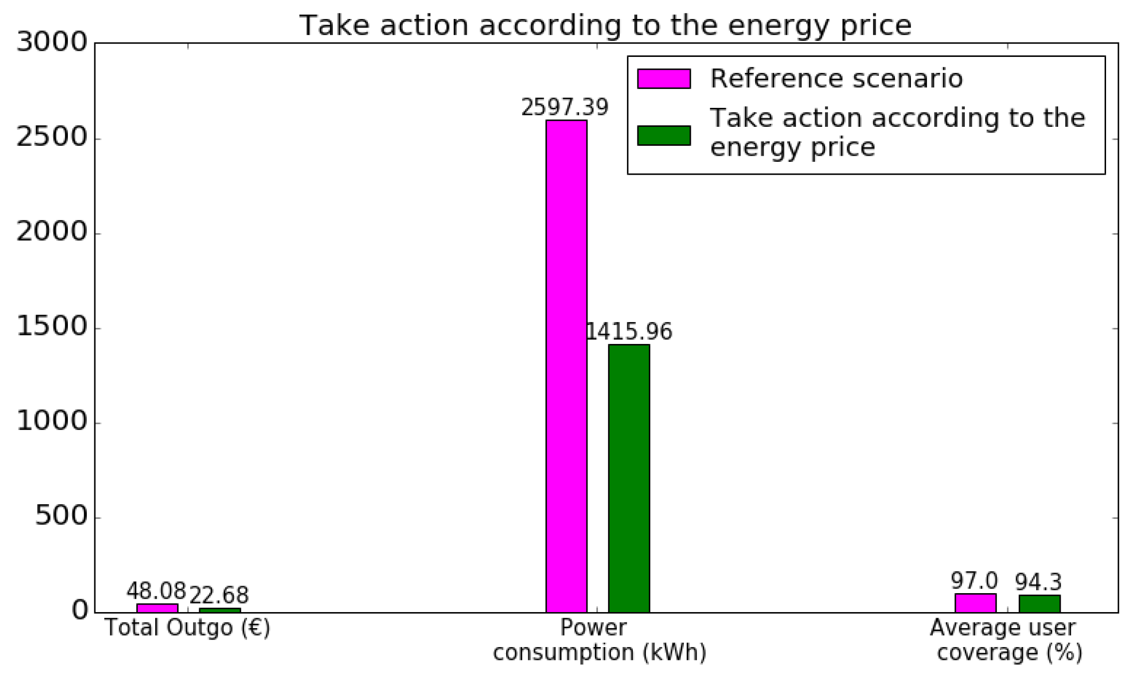
• it demonstrates that a careful analysis of the energy price provides the necessary energy cost reduction. The analysis determines when energy should be bought or when the power consumption should be reduced, according to the current energy price.

The outline of the paper is as follows. In Section 2, the methodology is discussed. Furthermore, the considered scenario and the cost-reducing strategies are described. Section 3 shows results obtained with them. Finally, in Section 4, the most important conclusions from this study and future work are summarized.

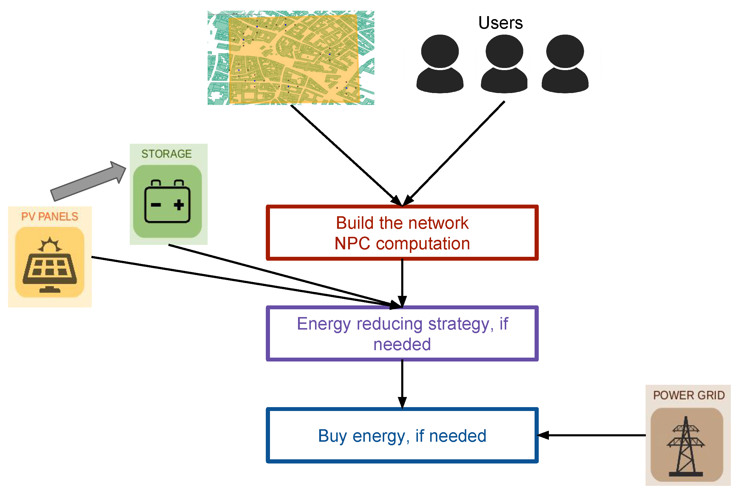
2. Materials and Methods

An LTE-A (Long-Term Evolution-Advanced) capacity-based wireless access network is considered. Capacity-based means that the network responds to the instantaneous bit-rate demand of active users in the considered area. The link budget parameters are summarized in

Table 1. Link budget parameters for the LTE-A macrocell and microcell base station.

Parameters	Macrocell Base Station	Microcell Base Station
Frequency	2.6 GHz
Maximum input power antenna	43 dBm	33 dBm
Antenna gain base station	18 dBi	4 dBi
Antenna gain mobile station	2 dBi
Soft hand over gain	0 dB
Feeder loss base station	0 dB
Feeder loss mobile station	0 dB
Fade margin	10 dB
Yearly availability	99.995%
Cell interference margin	2 dB
Bandwidth	5 MHz
Receiver SNR	1/3 QPSK = −1.5 dB, 1/2 QPSK = 3 dB, 2/3 QPSK = 10.5 dB, 1/2 16-QAM = 14 dB, 2/3 16-QAM = 19 dB, 4/5 16-QAM= 23 dB, 2/3 64-QAM = 29.4 dB
Used subcarriers	301
Total subcarriers	512
Noise figure mobile station	8 dB
Implementation loss mobile station	0 dB
Height mobile station	1.5 m
Coverage requirements	90%
Shadowing margin	13.2 dB
Building penetration loss	8.1 dB

. The considered area is 0.3 km${}^2$ of the suburban environment of the city center of Ghent, in Belgium (orange rectangle in Figure 1).

It is composed of a group of macrocell base stations and/or microcell base stations. It is powered with solar panels and equipped with batteries. The energy production of the PV panels is predicted with the data from [15]. The adopted trace reports data, provided on an hourly basis, about the power output obtained per each kWp of nominal capacity of the PV panel system. The values of renewable energy production are derived based on real data of solar irradiation in the considered area. They are observed in the week from 3 January–9 January during the typical meteorological year. In this way, the worst case scenario in terms of power generation is considered. These data are related to the city of Turin, since those of Ghent are not available. Energy losses due to the efficiency of PV modules and to the normal PV system operation are taken into account. For energy harvesting, lead-acid batteries represent a common technology adopted in renewable energy systems. A set of lead-acid battery units, each with a capacity of 200 Ah and a voltage 12 V, is hence assumed as storage in this work. Storage losses are neglected, occurring both during the battery charge and discharge and for the energy transfer and transmission. The energy generated by the panels is fed into the batteries, from which the base stations drain the energy. In case the batteries are discharged, the base stations are supplied by the traditional power grid. The renewable energy generator system of 100 kWp and the energy storage of 50 kWh are shared among all the base stations. The energy management decisions are made in a centralized way for all the base stations. In this way, decisions are based on the total available energy and the total power demand. The real-time pricing is considered for the energy prices, which are provided by the Belgian power operator [16]. They vary every hour, as shown in Figure 2.

Three different strategies are proposed, and different configurations are considered. Their performances are evaluated in terms of:

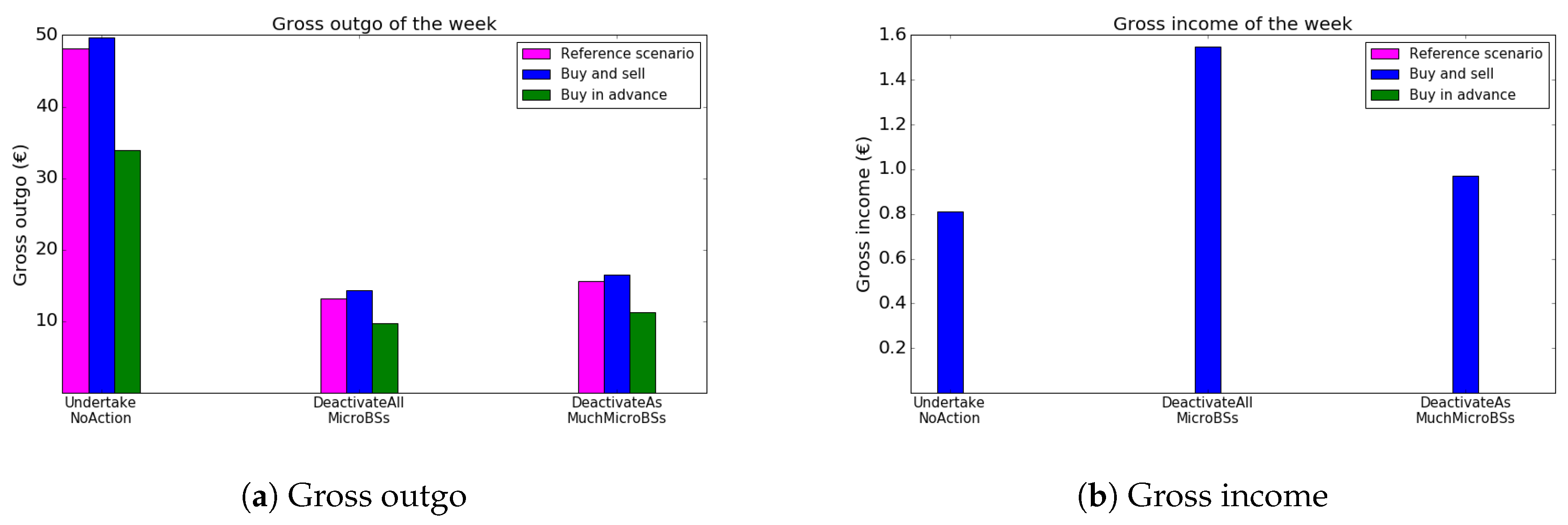
• gross outgo: this is the amount of money spent to buy energy from the power grid:

  $$total outgo=\sum _{k=1}^{N}energyBought\left[k\right]·energyPrice\left[k\right]$$

  (1)

  where N is the duration of the simulation (one week: 168 h or time intervals), energyPrice[k] is the energy price at the time interval k and energyBought[k] is the amount of energy bought at the instant k.
• gross income: this is the amount of money earned by selling energy to the traditional power grid;
• total outgo: this is computed as:

  $$total outgo=gross outgo-gross income$$

  (2)

Note that when the cost reducing strategy used does not consider the sale of the energy, the gross income is zero. Consequently, the total outgo is equal to the gross outgo. In these cases, only the total outgo is discussed.

2.1. Strategy 1: Simple Algorithms

In this case, the methodology of [14] is used and extended. The considered network is the real one of the city center of Ghent. It is composed of eight macrocell base stations (blue points in Figure 1), each supporting four microcell base stations (orange points in Figure 1). For each time slot (one-hour long), the number of active users is determined, using users’ predictions, built according to data provided by a mobile Belgian operator. Once the number of active users is known, the network can be determined: each user is associated with a base station, according to the algorithm used in [4], which aims at power consumption minimization (Step 1 in Figure 3).

At this point, as shown by the red step in Figure 4, the algorithm computes the power consumption of the network (NPC of Step 3 in Figure 3) for the current time interval (indicated with $t_i$ in Figure 3), using the power consumption model for macrocell and microcell base stations, described in [17].

The network’s power consumption is compared with the available energy, given the energy in the battery and the energy produced by the PV panels (respectively energy_stored[j] and energy_produced[j] in Step 4 in Figure 3). If the network consumes more than the available energy, one of the energy-reducing actions proposed and analyzed in [14] is applied (Step 7 in Figure 3 and the purple step in Figure 4):

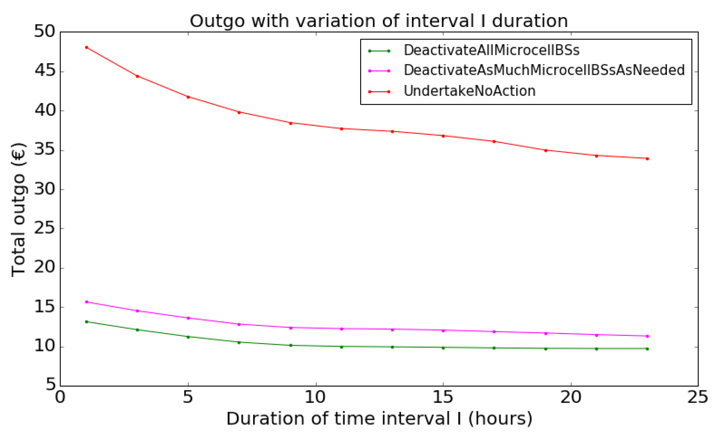
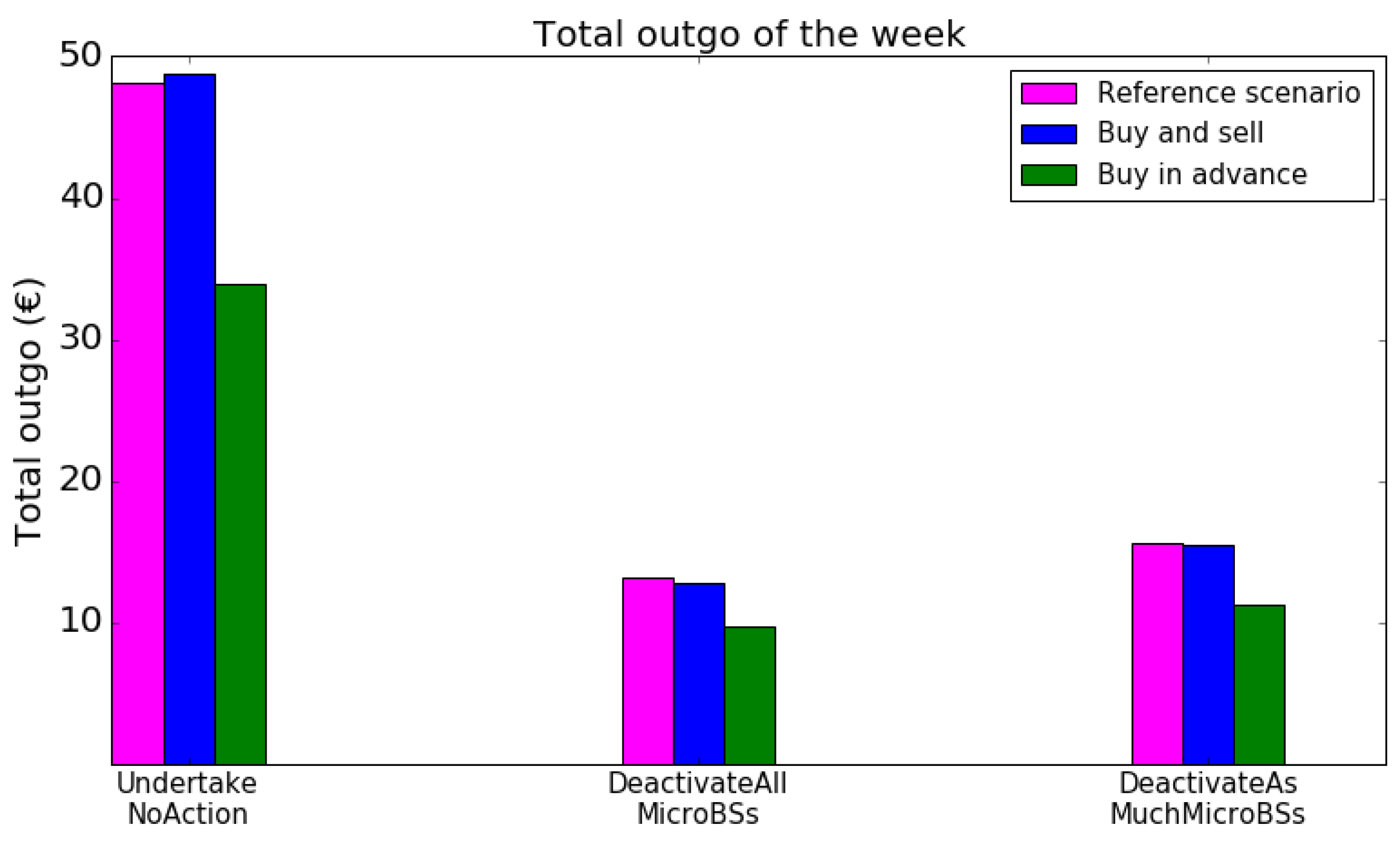
• Undertake no action: When using this, no adjustments are made at the network level. It represents the current situation. This is considered as the reference scenario, concerning the energetic aspect.
• Deactivate all microcell BSs: When this is used, all microcell base stations are turned off. When a base station is deactivated, its power consumption is assumed to be negligible. All users connected to these microcell base stations are reconnected to a macrocell base station, if possible.
• Deactivate as much microcell BSs as needed: This is a hybrid one; microcell base stations are turned off gradually. The network’s energy consumption is computed when switching off 1, 2 or 3 microcell base stations per macrocell base station. As soon as the network’s energy consumption becomes lower than the amount of available renewable energy, the necessary number of microcell base stations to be turned off is known. If turning off three microcell base stations is not sufficient, the previous strategy is applied. As in the previous case, all the users connected to the switched microcell base stations are reconnected, if possible.

The last two actions can be combined with a prediction time window TW, expressed in hours. Without considering the time window, the network’s energy demand and energy production for the current time interval are considered, and an energy action is applied in the case of energy shortage. When considering a time window, any energy shortage in the next few hours is taken into consideration. In particular, assuming a given time interval TI and a given time window TW, the time window period (indicated as TWPeriod in Figure 3) is defined as the period between TI and TI+TW (boundaries included). If an energy shortage is predicted during this, microcell base stations are switched off from TI, for the whole time window period duration.

Once the energy reducing action is applied, if the available energy continues to be insufficient, the amount of energy that cannot be provided by the PV panels and by the storage is bought from the traditional power grid (Step 8 in Figure 3 and the blue step in Figure 4). Therefore, the necessary energy cost and the energy storages are updated (Step 9 in Figure 3).

For this study, algorithms that aim at minimizing the total amount of money spent to buy the energy needed for the supply of base stations are introduced in the tool used in [14]:

• No action: When this is used, the energy is bought as soon as it is needed. This is the current situation and is considered as the reference algorithm.
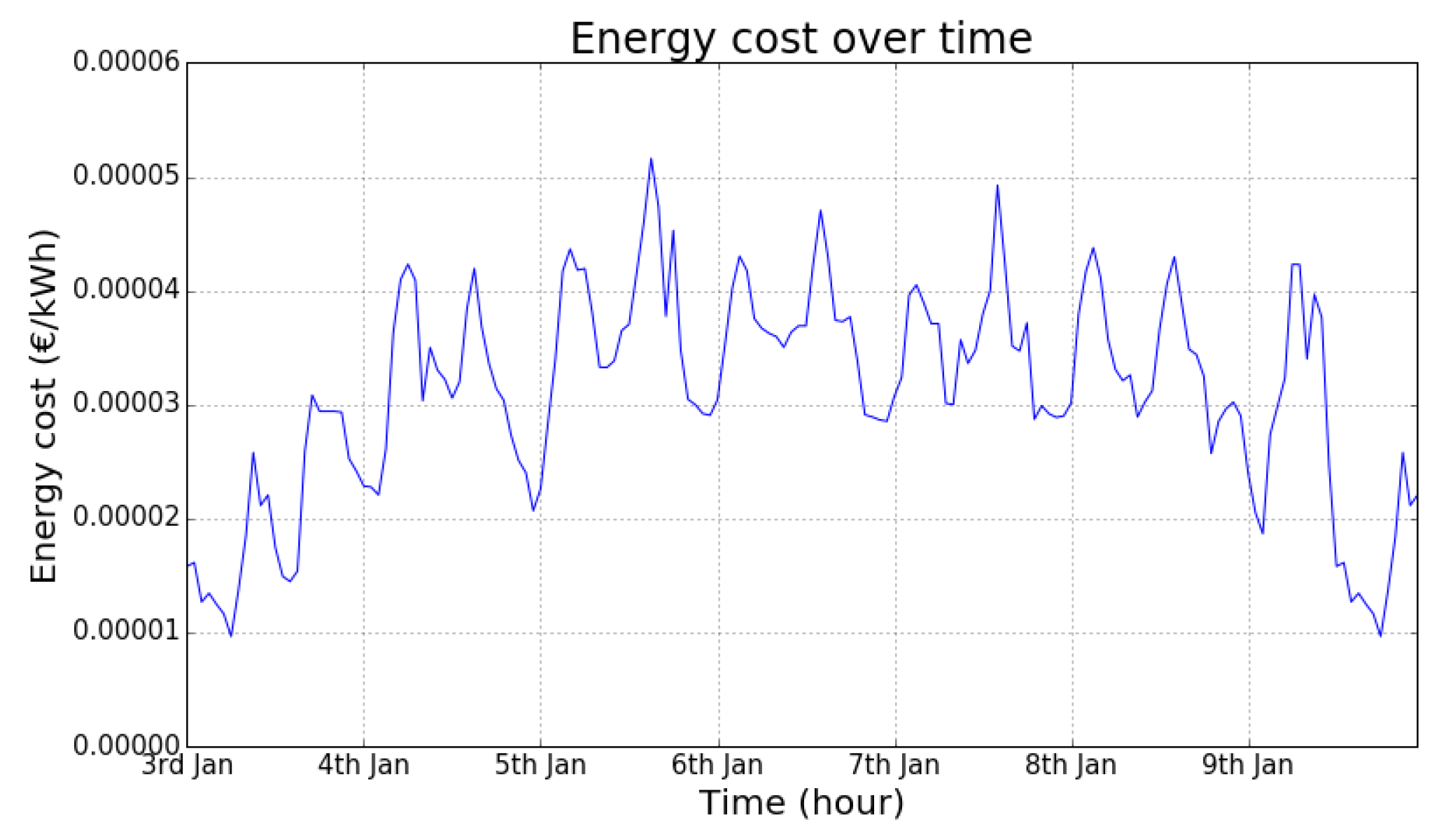
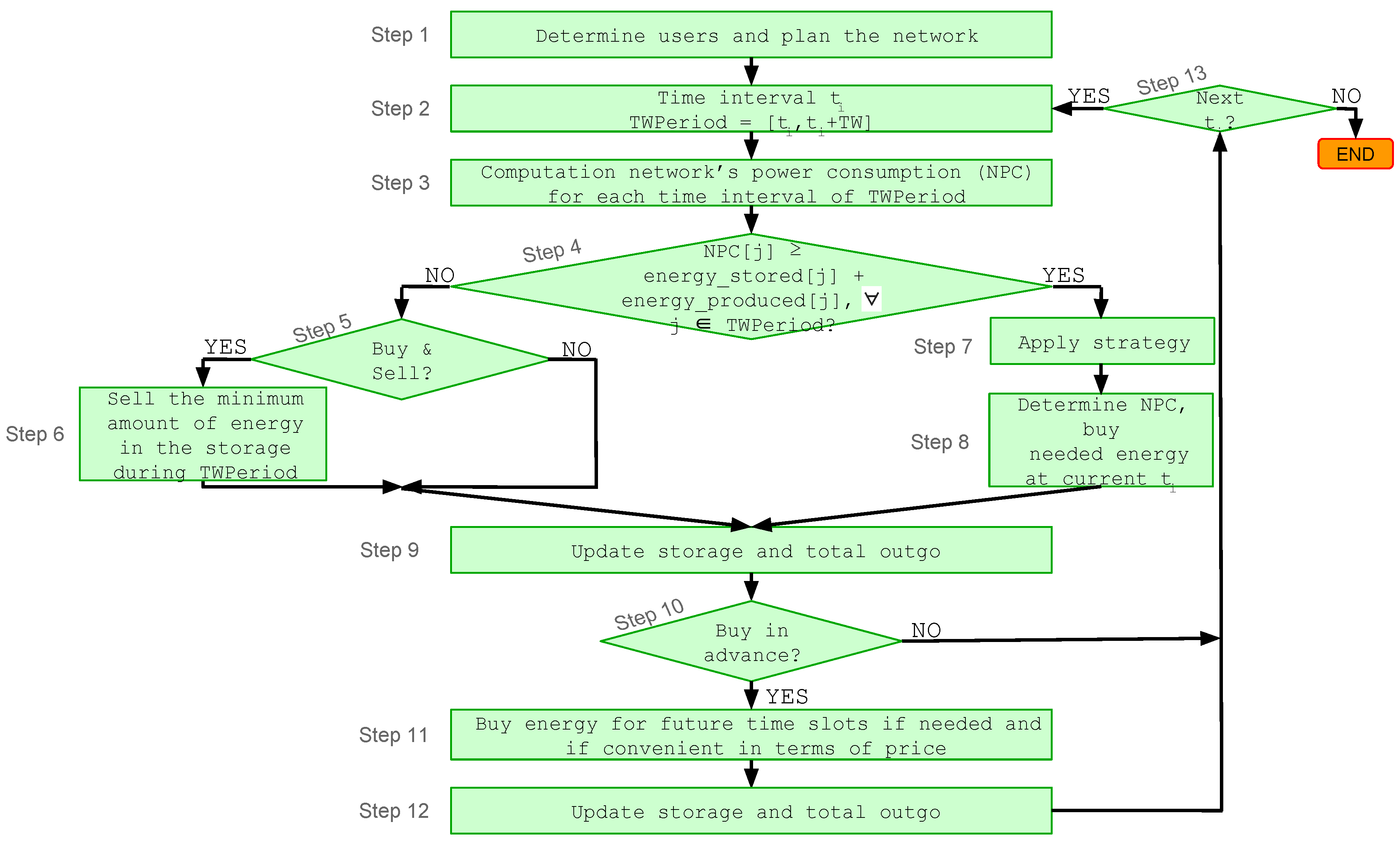
• Buy in advance: This algorithm tries to exploit the variation of the energy price during the day, reacting to the demand and response program. It is based on the idea that energy is not bought whenever it is needed, but when energy is less expensive. Therefore, it is stored in the energy batteries as long as it is not needed. This solution is widely exploited in the power community. Nevertheless, it is not used in the scenario considered in this study. The scenario that we are investigating is peculiar. In fact, the communication network cannot shift its load according to the energy price because the quality of service has to be always guaranteed. The network can not plan its usage, which depends on the users. This is not present in other applications. Moreover, this scenario is very suitable for this solution because of the already present energy batteries, installed for the power consumption minimization. Therefore, no additional Capex expenditure is required. The storage of produced energy is not compromised because network energy status forecasts are considered (Step 11 in Figure 3). In particular, at each time slot t, the algorithm iterates over a given number of the following time slots, and for each i of them, it defines:
  I: time period from t to i (I = [t,i]).
  If t is the time slot at the minimum energy cost in I and if i needs that energy to be acquired (predicted stored and produced energy is not sufficient for that time interval), the definition of variable bought occurs as follows:

  bought: 

  energy that can be bought at t. It is the minimum space available in the storage from t up to i. In this way, we avoid that produced energy in the following time interval that should be stored in the battery is wasted, because of the presence of the bought one.

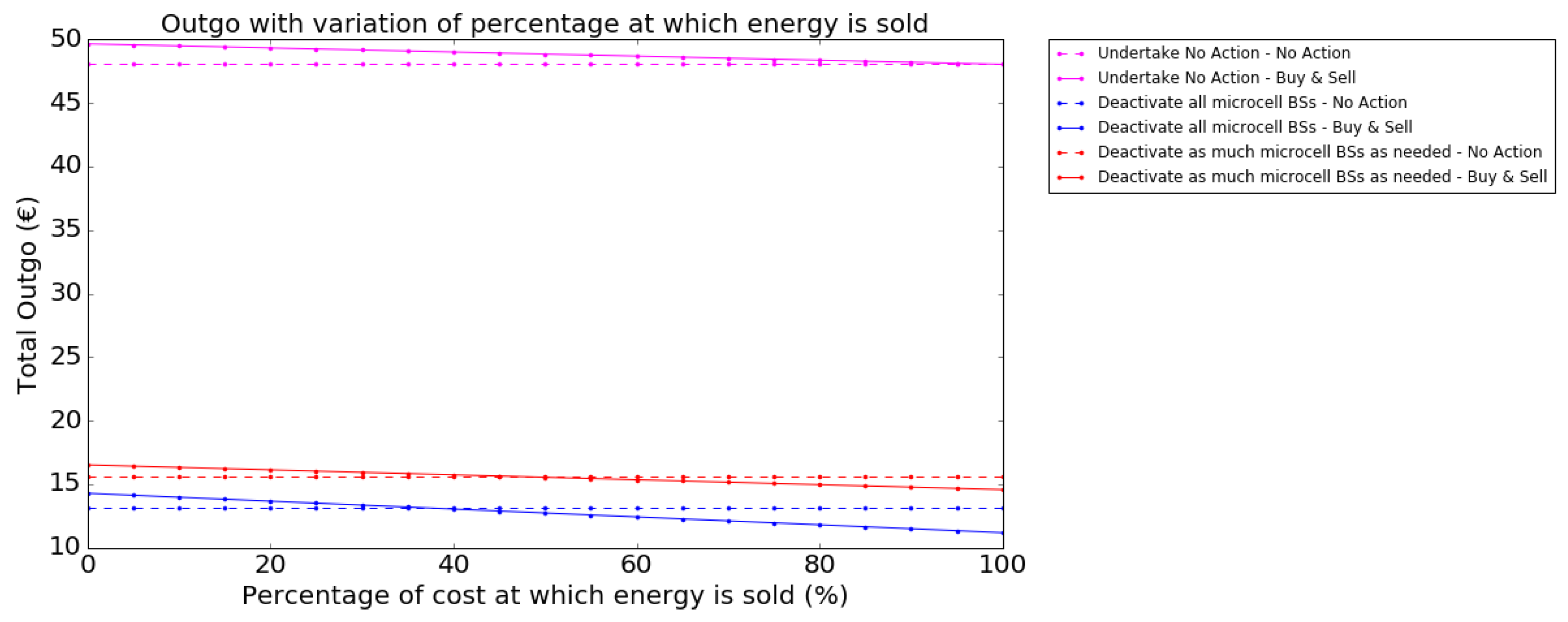
  Therefore, the bought amount of energy is taken from the grid at time slot t and stored in the batteries. In case the amount of energy bought during past time slots and allocated for the current one is not sufficient, the necessary amount is purchased from the power grid.
  The number of time slots over which the algorithm iterates (maximum duration of time interval I) is a parameter that is investigated in this study. Nevertheless, its maximum value is 23 h since that amount of time is indicated in the literature as the maximum time of storage to avoid substantial energy losses. This algorithm does not affect network parameters since it acts in a transparent way for the communication system.
• Buy and sell: the solution exploits the fact that base stations are prosumers. In fact, they consume and produce electrical energy from their solar panel. This action makes the access network an active participant in the energy market: the network does not only buy and take energy from the traditional power grid, but also sells and injects energy into it.
  The energy is sold when the access network is not in a critical situation (Steps 4–6 in Figure 3): this is the condition in which energy strategies are not applied. Therefore, when the critical situation does not occur, at the current time interval t, microcell base stations are not switched off because the amount of produced and stored energy is sufficient for the base stations supply for that time interval t and for all the time intervals belonging to the time window period. In this way, the sale and immediate purchase of energy are avoided. Preventing this kind of situation is convenient because energy is sold at a lower price than the one at which it is bought.
  The amount of energy sold is equal to the minimum amount of energy remaining in the storage for the time slots belonging to the time window period. Therefore, it is the quantity of electricity that is exceeded during the considered time period. Concerning energy sale price, in the literature, nothing is presented. For this reason, the percentage of the purchase price at which the energy can be sold is investigated.
  This solution is the one and only case for which the gross income is different from zero, since only in this case, the sale of energy is allowed.
  The purchase of energy is done as soon as needed. This policy does not affect the network parameters.

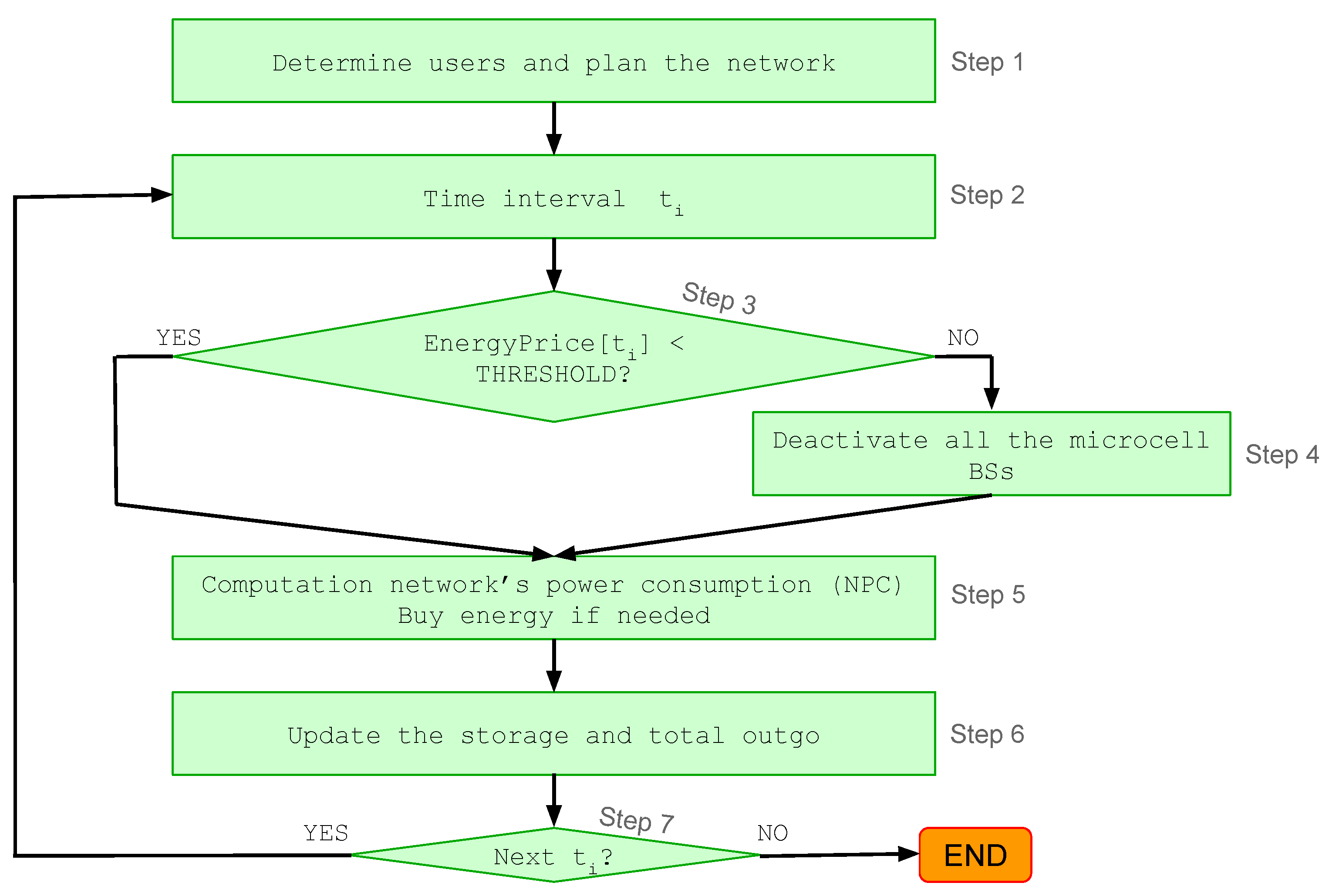
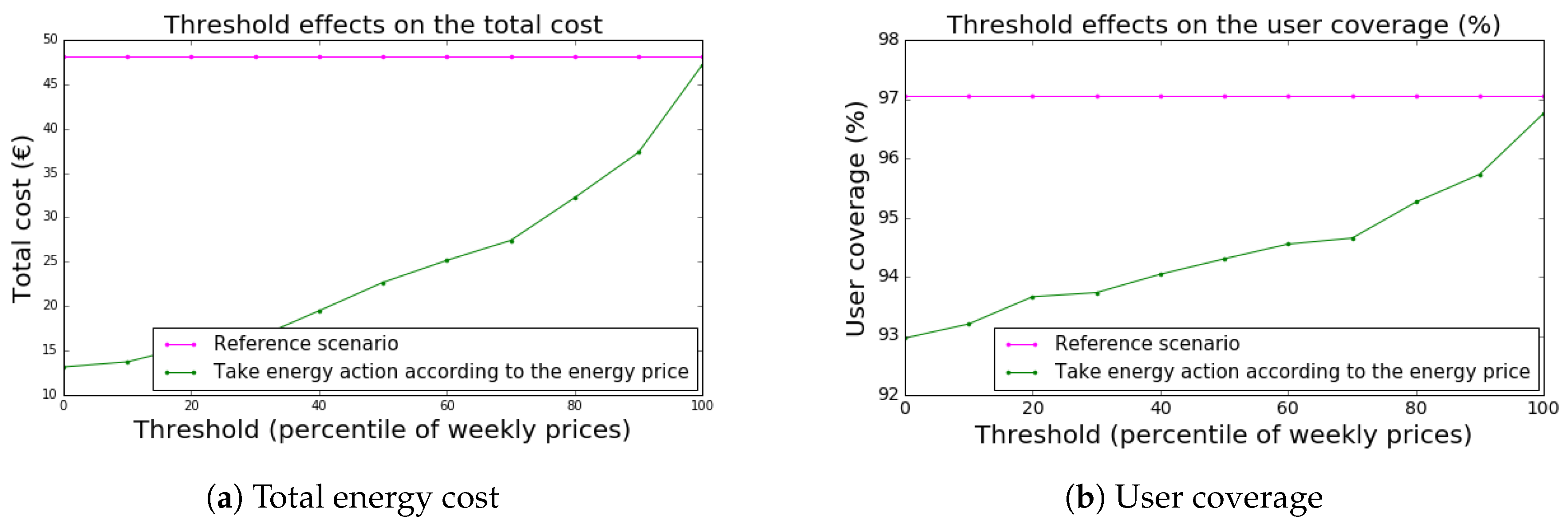
2.2. Strategy 2: Take Action According to the Energy Price

This strategy exploits the variability of the energy prices and the reduction of the necessary energy cost through the power consumption drop. The idea is to reduce the energy consumption during energy peak price hours. In particular, once the number of active users is determined and the network is built as described in [14] (Step 1 in Figure 5), with the already mentioned network configuration (Figure 1), the hourly energy price is checked (Step 3 in Figure 5). If it is higher than (or equal to) a given threshold, all microcell base stations are switched off (Step 4 in Figure 5). Then, if the available energy is not enough for the supply of the base stations at the current time interval, the missing part of power is bought from the traditional power grid (Step 5 in Figure 5). Therefore, the total necessary energy price and the storage are updated (Step 6 in Figure 5).

The threshold parameter is investigated in this study. It is expressed in terms of the level of the percentile of the weekly energy price.

Note that the high energy price usually occurs during day time, when many users are active (Figure 2). For this reason, it is important to verify that the quality of service remains good.

This strategy can be combined with the prediction time window TW. In case a time interval in the time window period has an energy price greater than (or equal to) the threshold, all microcell base stations are deactivated. Therefore, more energy is saved, and a lower quantity of it will be bought during that time interval.

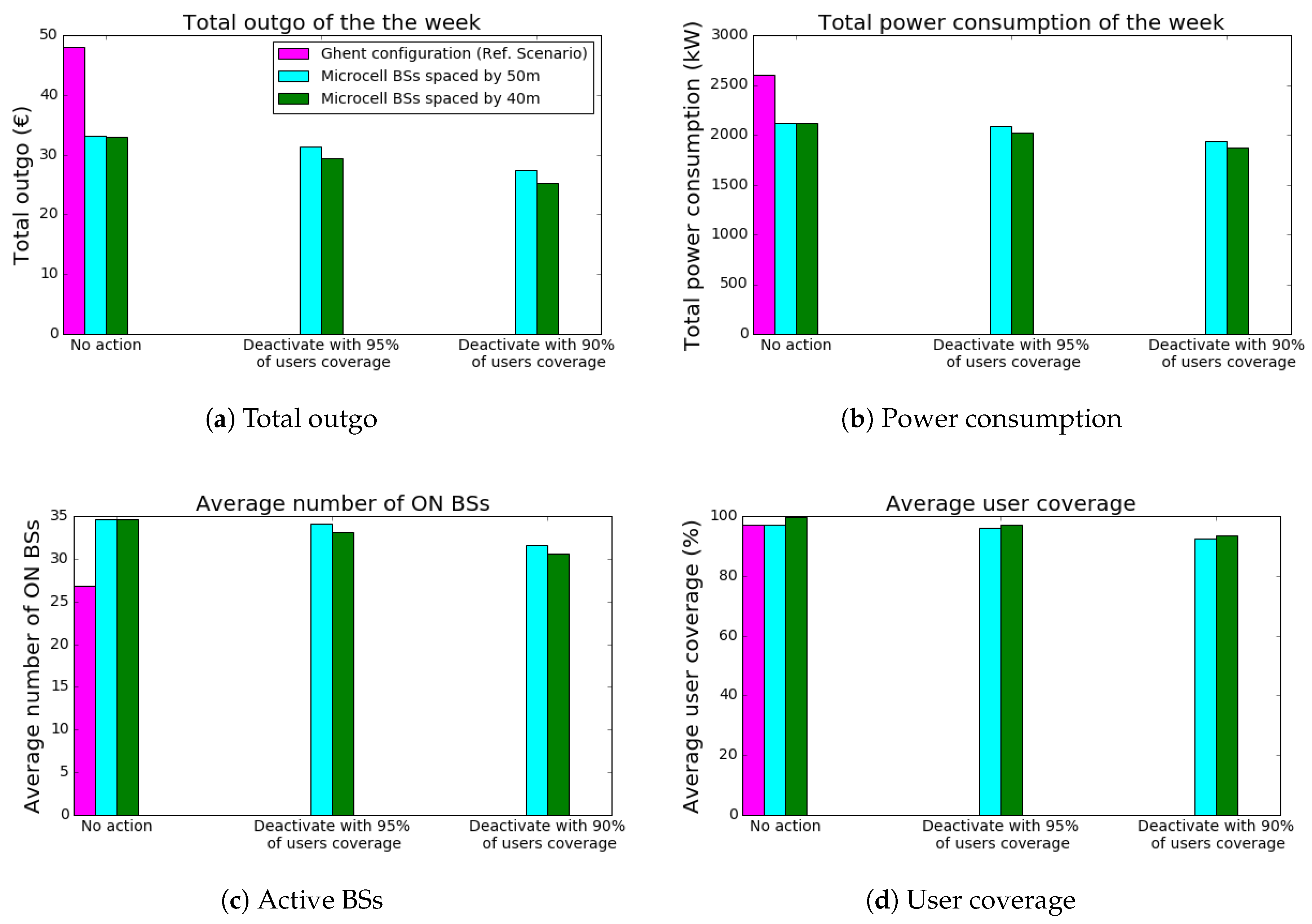
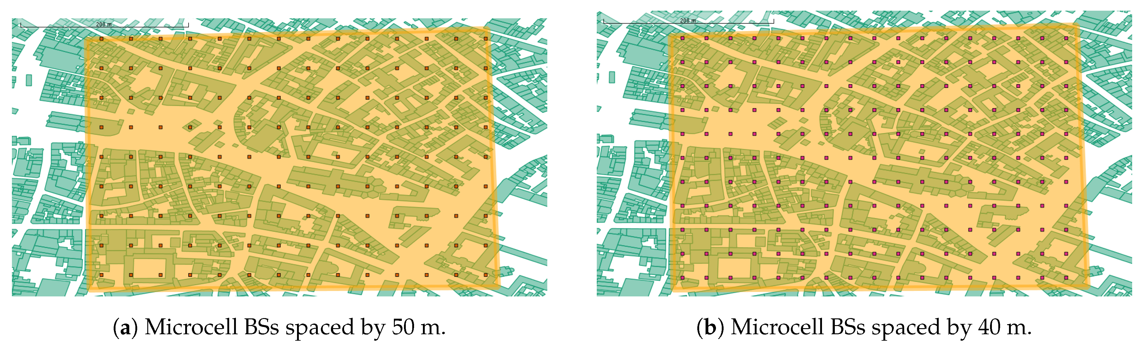
2.3. Strategy 3: Microcell BSs Networks

In this method, energy expenditure is reduced by the reduction of the power consumption. The microcell base stations are lower power consumers than macrocell base stations, as claimed in [5]. Therefore, two new configurations, composed by microcell base stations only, are proposed. The presented configurations are obtained by placing the microcell base stations in equispaced points on the considered area (base stations are assumed to be points), at a 1.5-m height:

• base stations are spaced by 50 m horizontally and vertically: for the considered area of 0.3 km${}^2$ of the city center of Ghent, 126 microcell base stations are needed (Figure 6a);
• base stations are spaced by 40 m horizontally and vertically: 187 microcell base stations are used (Figure 6b).

The horizontal and vertical distances at which base stations are placed (50 m and 40 m) are chosen arbitrarily, taking into consideration the radio range of the used infrastructures, aiming at minimizing the uncovered area. The cell interference margin of the link budget (Table 1) is approximated as 4 dB and 5 dB for the configuration with base stations spaced by 50 m and 40 m, respectively.

Once the number of active users is known, the network is built considering one of the two configurations previously described, using the algorithm developed in [4] (Step 1 in Figure 7). Then, the power consumption is computed, and it is compared with the available energy (stored and produced). In case the needed energy is greater than that available, one of the two following energy-reducing actions is applied:

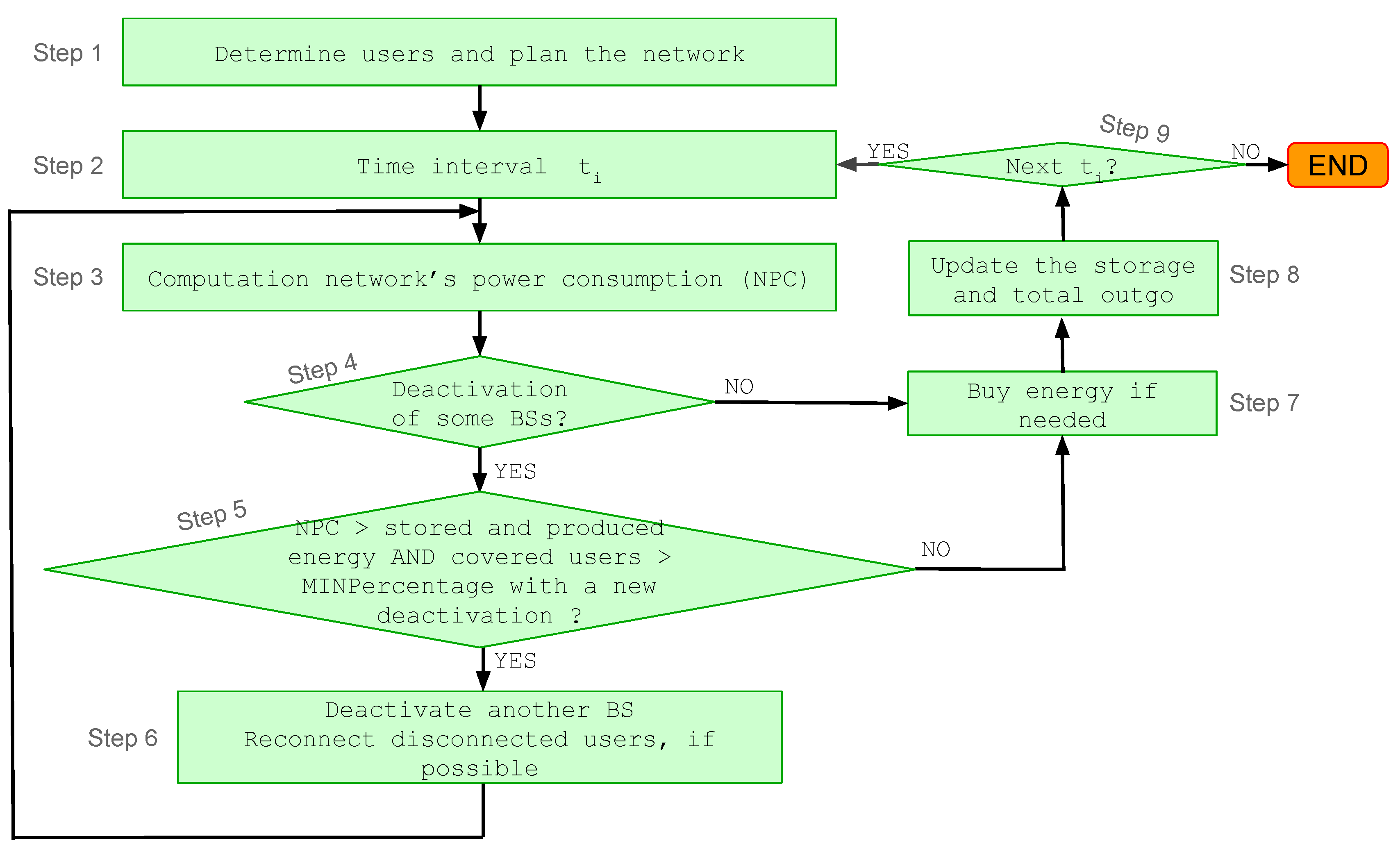
• Only Microcell BSs: No Action: In this case, no action is performed. It is used to check the effects of the new proposed configurations. If the available energy is not sufficient to power the base stations, the missing amount is purchased from the electricity grid (Step 7 in Figure 7). The storage and the total necessary energy cost are updated (Step 8 in Figure 7).
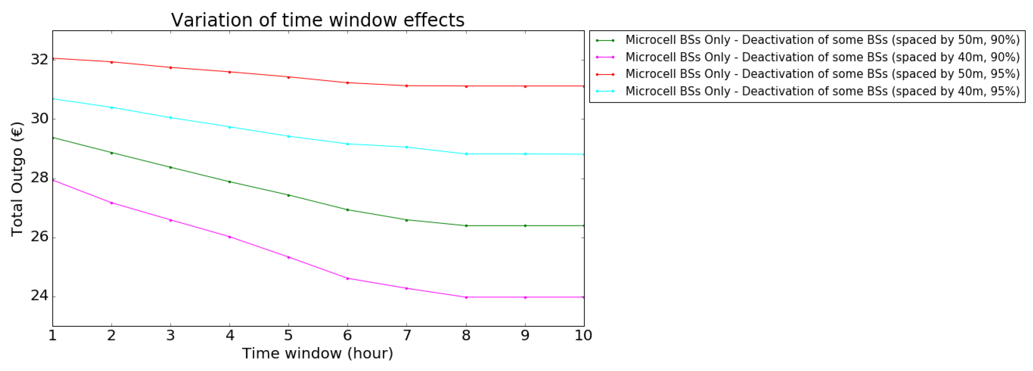
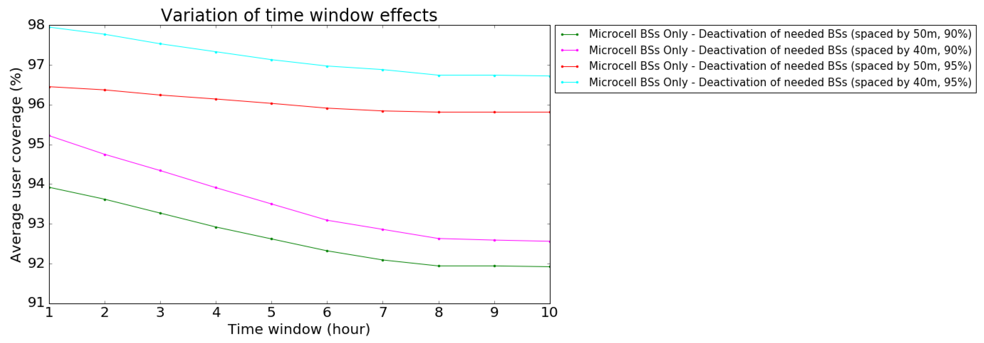
• Only Microcell BSs: Deactivation of some BSs: A part of the microcell base stations is turned off gradually in the event of an energy shortage. The energy consumption of the access network is computed when switching off 1, 2, 3,…,N microcell base stations. As soon as the network’s energy consumption becomes lower than the amount of available renewable energy (stored and produced energy), the necessary number of microcell base stations to be turned off is known.
  Since the power consumption of a microcell base station is low, many of them should be switched off. In this way, the capacity of the network can be compromised. For this reason, base stations can be deactivated until a minimum percentage of users is covered. The solution is tested with 95% and 90% guaranteed user coverage (Step 5 in Figure 7). All the users connected to the switched microcell base stations are reconnected, if possible (Step 6 in Figure 7). If the available energy continues to be insufficient for the base stations’ supply, the missing part is bought from the traditional power grid (Step 7 in Figure 7). The necessary energy cost and the energy storage are updated (Step 8 in Figure 7).
  The strategy can be combined with the time window TW: when an energy shortage is detected in a time slot belonging to the time window period, the necessary microcell base stations are deactivated.

The network performance parameters are also discussed for this strategy.

3. Results and Discussion

In this section, the evolution of the total cost for the necessary energy to supply the base stations during one week is investigated, applying the methodologies described in the previous section.

As already mentioned, the worst week of the year in terms of solar power generation is considered: from 3–9 January.

Parameters are set in the following way (unless mentioned otherwise), as suggested in [14]:

• PV panel capacity: 100 kWp;
• storage capacity: 50 kWh;
• time window TW, when present: 5 h.

The reference scenario corresponds to the current situation: neither an energy-reducing action, nor a cost-reducing action are used (Undertake no action and No action of Strategy 1) in the wireless access network equipped with a PV panel system and energy batteries described above.

3.1. Results: Strategy 1, Simple Algorithms

The results obtained with the cost-reducing actions of Strategy 1 (Section 2.1) are shown in Figure 8. Concerning Buy in advance, the interval I is set to 23 h. For Buy and sell, the energy is sold at the half market price. The remaining parameters are set as previously mentioned.

Note that the Buy in advance algorithm provides considerable reduction in terms of total energy cost. The scenario in which Undertake no action is used presents the largest reduction (until approximately 30%, Figure 8). In this case, the storage is on average 52% and 65% less full than for Deactivate as much microcell BSs as needed and Deactivate all microcell BSs, respectively. Therefore, the algorithm can be more effective since a larger amount of energy can be bought in advance, if the energy is less expensive. This explains also the difference concerning the reduction of cost when the two different energy-reducing actions are used, which provide 27.7% and 26% cost reductions, with Deactivate as much microcell BSs as needed and Deactivate all microcell BSs, respectively.

With respect to Buy and sell, reductions are not large (Figure 8) and not always achieved: the cost increases by 1.5%, when Undertake no action is used. A 3% and less than 0.7% reduction is obtained with Deactivate all microcell BSs and Deactivate as much microcell BSs as needed, respectively. These results are summarized in

Table 2. Table with the summary of the most significant results. In Strategy 1 (Buy in advance and Buy and sell algorithms), results are reported for each energy reducing strategy: 1 is Undertake no action; 2 is Deactivate all microcell BSs; 3 is Deactivate as much microcell BSs as needed. The parameters setting is indicated in the table.

Strategy 1: Simple Algorithms TW = 5 h; Panel Capacity = 100 kWp
Buy in advance; I duration = 23 h; Storage capacity = 60 kWh
Gross outgo (€)			Gross income (€)			Total outgo (€)			Total outgo drop (%)
1	2	3	1	2	3	1	2	3	1	2	3
33.80	8.68	11.30	0	0	0	33.80	8.68	11.30	29.53	28.86	27.65
Buy and sell; Price of sale of energy = 50% of market price; Storage capacity = 50 kWh
Gross outgo (€)			Gross income (€)			Total outgo (€)			Total outgo drop (%)
1	2	3	1	2	3	1	2	3	1	2	3
49.64	14.29	16.52	0.81	1.55	0.97	48.83	12.74	15.55	−1.56	3.12	0.69
Strategy 2: take action according to the energy price Threshold = 70th percentile; TW = 5 h
Gross outgo (€)		Gross income (€)		Total outgo (€)		User coverage (%)		Total outgo drop (%)		User coverage drop (%)
27.41		0		27.41		94.65		42.99		2.47
Strategy 3: microcell BSs networks TW = 4 h; Storage capacity = 50 kWh; PV panel capacity = 100 kWp
Strategy		# BSs	Ensured use coverage (%)		Gross outgo (€)	Gross income (€)	Total outgo (€)	User coverage (%)	Total outgo drop (%)	User coverage drop (%)
No action		126	-		33.06	0	33.06	97.31	31.23	−0.31
No action		187	-		32.91	0	32.91	99.81	31.55	−2.89
Deactivation of some BSs		126	90		27.88	0	27.88	92.92	42.01	4.22
Deactivation of some BSs		126	95		31.60	0	31.60	96.14	34.28	0.90
Deactivation of some BSs		187	90		26.02	0	26.02	93.91	45.88	3.2
Deactivation of some BSs		187	95		29.74	0	29.74	97.33	38.14	0.33

.

Drops are limited since the amount of money spent to buy the necessary energy is greater (Figure 9a) than when the energy is not sold. This is due to the fact that the amount of sold energy is actually needed for the base stations’ supply. For this reason, it is bought back, often at a higher price than the one at which it has been sold.

The amount of money earned thanks to the energy sale (Figure 9b) contributes to the reduction of the total outgo. The gross income is larger when an energy-reducing action is applied since, in those cases, the network is more often out of the critical situation, and so, it can sell electricity. In case no energy-reducing strategy is used, the sold energy is not enough to make the total outgo lower than the reference scenario.

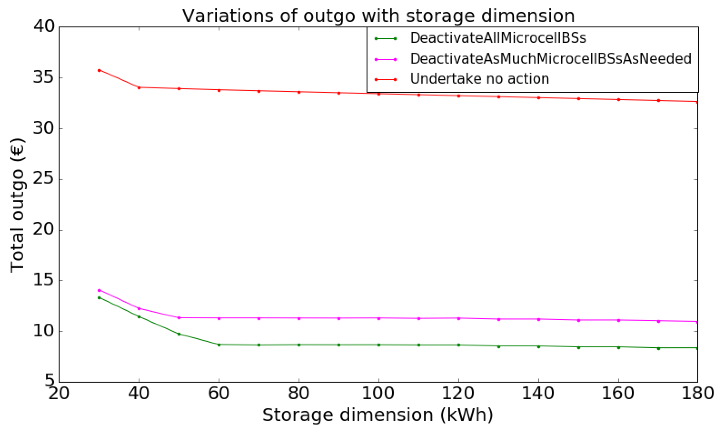
3.1.1. Buy in Advance: Storage Dimension and I Interval Maximum Duration Effects

Considering the observations made above, it is interesting to perform simulations, varying the energy storage capacity, when Buy in advance is used.

The results are shown in Figure 10, varying the storage capacity from 30 kWh–180 kWh.

Note that, as the energy storage capacity increases, money spent to buy energy from the grid decreases, since more energy can be bought in advance, when it has a lower price. When Deactivate all microcell BSs is used, the slope of its decrease reduces at approximately 60 kWh. In fact, with an energy storage of 30 kWh, total cost is reduced by approximately 23%, while when it is 60 kWh, by approximately 28.86% (as shown in Table 2), and no additional reductions are obtained for storages greater than 80 kWh. In the scenario in which Deactivate as much microcell BSs as needed is used, the total cost starts to stabilize at 50 kWh: with 30 kWh, the reduction is approximately 22.5%, while 27.65% with 60 kWh, as shown in Table 2, but no significant additional reductions are obtained for larger storage capacities. These interruptions in the decreasing trends are because the total cost is close to the minimum price needed to buy all the necessary energy. If we suppose to buy ideally all the necessary energy during the time interval at the minimum price, between €3 and €3.5 are necessary, according to the energy policies used. When no energy reducing action is used (Undertake no action), the total cost continues decreasing linearly, even with a smaller slope from 40 kWh on, since it is still far from the minimum total cost (approximately €11).

Next, simulations are performed changing the duration of the interval I. This parameter refers to the maximum number of hours (time intervals) for which energy can be bought in advance, if needed and if it is less expensive. Simulations are done using I interval duration values varying from 1–23 h (time intervals). The results are shown in Figure 11.

For a duration of I = 1 h, the cost is very high since this scenario actually coincides with the one in which the reducing cost algorithm is not used. Increasing the duration of the interval I, the algorithm behaves better since it is more likely to buy energy during the time slot that is the local minimum among hourly costs. As in the previous analysis, the stability is reached after I duration equal to 9 h, when Deactivate all microcell BSs and Deactivate as much microcell BSs as needed are used. Increasing its duration from 1–7 h, the cost is reduced by 19% and 18%, respectively. However, with I equal to 11 h, costs are further reduced by less than 5% only. This is explained by the storage saturation: the storage becomes full so that the purchase of energy for more future time intervals is not possible. With Undertake no action, saturation does not occur since the storage is more empty because of the larger power consumption in that scenario. Consequently, the total outgo continues decreasing even with great values for the duration of the interval I.

3.1.2. Buy and Sell: Percentage of Price Evaluation

The price at which energy should be sold in order to obtain cost reduction is investigated. This is done in terms of a percentage of the market energy price. In Figure 12, the total outgo is plotted varying this percentage.

As already mentioned, the sale of energy at 50% of its market price provides a very limited reduction of cost when different energy-reducing actions are applied: with Deactivate all microcell BSs, costs are reduced by 3%, while with Deactivate as much microcell BSs as needed, by less than 1%, with respect to the scenarios with the same energy-reducing action and No action as the cost-reducing one. When the energy is sold at 75% of the market price, reductions are approximately 9% and 4%, respectively. In case energy reducing actions are not used, even selling energy at 90% of its market price does not reduce costs because of the reasons already mentioned: the system is not sufficiently out of the critical situation to obtain cost reductions by the sale of the energy.

3.2. Results: Strategy 2 Take Action According to the Energy Price

In this part, results obtained with Strategy 2 are presented. Simulations are performed setting the 50th percentile of the hourly energy price during the considered week as the threshold of Take action according to the energy price. As shown in Figure 13, the introduction of the proposed strategy reduces cost by more than 52%, from €48.08–€22.68, since the energy consumption is lower (Figure 13). In fact, the total power used drops by more than 45% with respect to the reference scenario. Nevertheless, the average user coverage is reduced by less than 3% (Figure 13).

Take Action According to the Energy Price: Threshold Effects

In Figure 14a, the total energy cost is shown, varying the threshold used for the deactivation of the microcell base stations. The threshold parameter is investigated in terms of the percentile of the hourly energy price during the week. Increasing its value (increasing the percentile), the total cost increases as well, since the energy price is less often greater than it. Therefore, the energy consumption of the network increases and consequently the total energy cost. At the same time, the increase of the analyzed parameter acts in favor of the user coverage (Figure 14b), since base stations are less likely to be deactivated.

In fact, with threshold values lower than the 30th percentile, more than a 65% cost reduction can be achieved, but this results also in a user coverage drop of more than 3.42%. When the threshold is equal to the 70th percentile, the total outgo drops by approximately 43% and the user coverage by 2.47%, as summarized in Table 2. With values higher than the 80th percentile, the users coverage drop is limited to approximately 1.8%, but with cost reductions lower than 33%.

3.3. Results: Strategy 3 Microcell BSs Networks

Figure 15 shows the results for the strategy microcell BSs networks. The introduction of the configurations composed by microcell base stations only provides some benefits in terms of cost reduction (Figure 15a): their usage provides a total cost reduction of more than 31%, with respect to the reference scenario (Table 2).

The difference in terms of necessary energy cost between the case with 187 microcell base stations and the one with only 126 microcell base stations is negligible (less than 1%). Consequently, the total power consumption is similar, as well (Figure 15b), to the number of active base stations (Figure 15c). In the reference scenario, the number of active base stations is lower, but the presence of macrocell base stations contributes significantly to the total power consumption. The average user coverage is larger when the base stations are spaced by 40 m (187 microcell base stations usage): 99.81% in this case, while approximately 97% in the reference scenario and when the distance between the base stations is 50 m. This is because in the configuration with 187 microcell base stations, more redundancy is introduced, and therefore, a higher number of users can be served.

When the deactivation of base stations is possible, in case of an energy shortage, the increase of the minimum percentage of covered users implies the increase of the total outgo. This is caused by the higher quantity of required power (Figure 15b) due to the higher number of active base stations (Figure 15c) necessary to provide the required user coverage. In fact, it is possible to achieve more than a 38% reduction of total outgo, when at least 95% of users are always covered, and up to 47.32% when the minimum user coverage required is 90%, in the scenario with microcell base stations spaced by 40 m. In case 126 microcell base stations are used, more than a 34% and an approximately 43% cost reduction are obtained, when the minimum user coverage is 95% and 90%, respectively. The user coverage is reduced, but not compromised, since it is always larger than 92.5% (Figure 15d).

Only Microcell BSs: Deactivation of Some BSs (Time Window Effects)

Simulations are performed changing the time window value in Only Microcell BSs: Deactivation of some BSs. This varies from 1–10 h. Figure 16 shows that the total outgo decreases for increasing durations of this parameter, at the expense of the user coverage reduction (Figure 17).

This is due to the fact that with the growth of the time window, microcell base stations are deactivated more in advance so that more energy is saved. Consequently, a smaller quantity of electricity needs to be bought, but a lower percentage of users can be served.

With the time window equal to four, when 90% of users are always served, the total outgo is reduced by 42.01% (50-m BS spacing), with respect to the reference scenario, and by 45.88% in the case of 40 m between two base stations. This causes a user coverage drop of 4.22% and 3.2%, respectively. Nevertheless, the user coverage is acceptable since it is always greater than 92.92%. In case the percentage of served customers needs to be at least 95%, then more than 38.14% of the total outgo is saved, with 187 microcell base stations (40 m spacing) and more than 34% with 126 microcell base stations (50-m spacing), decreasing the coverage of the users compared to the reference scenario by less than 1%. These results are summarized in Table 2.

The reduction stabilizes: at a time window equal to 8 h when base stations are spaced by 40 m and at a time window equal to 7 h for base stations spaced by 50 m. This is because from that value, an energy shortage is always predicted, and so, the network starts acting always in the same way, reacting to the lack of renewable energy every time interval.

4. Conclusions

During the last few years, data traffic demand has increased greatly, as has the energy price. Wireless access networks have expanded, as well, in terms of size and provided capability and, consequently, in terms of power consumption. For this reason, the cost to buy the amount of power consumed by the base stations of those networks has become very high, impacting the communication cost. The goal of the paper is to design strategies and algorithms to minimize the total outgo for the purchase of the needed electricity for the supply of the base stations of a wireless access network. The network considered is an energy-efficient network, composed of a group of macrocell and/or microcell base stations, powered by a solar panel system, energy batteries and the traditional power grid. Exploiting the variability of the energy prices (real-time pricing is considered) reduces the total cost. When energy is bought in advance, if it is less expensive, the cost reduction is between 4.83% and 37.36%, when a 100-kWp PV panel system is used. The value of the cost reduction depends on the considered energy reducing strategies, the settings of the energy storage system and the parameter I. Recommended values for the interval duration I, during which energy can be bought in advance, are between 9 and 23 h. Regarding the storage capacity, the best value is around 60 kWh. The necessary energy cost is also reduced, when microcell base stations are switched off in case the energy price is greater than a given threshold. The value of the reduction depends on the setting of this threshold. Nevertheless the network performance worsens. For this reason, a compromise between the reduction of cost and the quality of service is needed. Therefore, the recommended value of the threshold is the 70th percentile. When the network is equipped with a 100-kWp PV panel system and a 50-kWh energy battery, an approximately 43% cost drop is achieved. The user coverage is reduced by less than 2.5%, but it remains larger than 94%, which is still acceptable as operators aim for 90% user coverage at least.

In these cases, the obtained benefits are in terms of energy cost reduction, but also in terms of the reduction of greenhouse gas emissions since the access network responds as expected to the demand and response program; therefore, it contributes to minimizing the peak power demand.

Next, the energy sale is introduced. With this strategy, the obtained results are not very promising since the sold energy has to be bought back: no more than a 3% cost reduction is obtained, selling energy at half of its market price.

Finally, the usage of a wireless access network composed of only microcell base stations is proposed. Since its power consumption is reduced, also the total necessary energy cost decreases. When a 50-kWh energy battery and a 100-kWp PV panel system are used, up to a 31% reduction of cost is achieved, without negative effects on the user coverage. However, the new configurations require a huge Capex expenditure due to the high number of base stations needed to provide a good quality of service. Performances can be further improved with the turning off of some base stations, in the case of renewable energy shortage. Nevertheless, this impacts the quality of service. Therefore, a compromise between the reduction of cost and the network performance is necessary. The suggested value for the time window is 4 h. When a 50-kWh energy storage and a 100-kWp PV panel system are used, an energy cost reduction between 34.28% and 45.88% is provided, with a user coverage drop between 0.33% and 4.22%, depending on the chosen configuration and the minimum ensured user coverage. This network parameter remains larger than 92.92%.

As future work, different energy pricing methods and different renewable energy resources will be considered. Furthermore, it could be interesting to improve the sale of energy: when the price is higher, injection should be performed.

References

1. CISCO. The Cisco® Visual Networking Index (VNI) Global Mobile Data Traffic Forecast; CISCO: San Jose, CA, USA, 2017. [Google Scholar]
2. Pickavet, M.; Vereecken, W.; Demeyer, S.; Audenaert, P.; Vermeulen, B.; Develder, C.; Colle, D.; Dhoedt, B.; Demeester, P. Worldwide Energy Needs for ICT: the Rise of Power-Aware Networking. In Proceedings of the 2nd International Symposium on Advanced Networks and Telecommunication Systems, Bombay, India, 15–17 December 2008; pp. 1–3. [Google Scholar]
3. Lambert, S.; Deruyck, M.; Van Heddeghem, W.; Lannoo, B.; Joseph, W.; Colle, D.; Pickavet, M.; Demeester, P. Post-peak ICT: Graceful degradation for communication networks in an energy constrained future. IEEE Commun. Mag. 2015, 53, 166–174. [Google Scholar] [CrossRef]
4. Deruyck, M.; Joseph, W.; Tanghe, E.; Martens, L. Reducing the power consumption in LTE-Advanced wireless access network by a capacity based deployement tool. Radio Sci. 2014, 49, 777–787. [Google Scholar] [CrossRef]
5. Patel, C.; Yavuz, M.; Nanda, S. Femtocells [Industry Perspectives]. IEEE Wireless Communications 2010, 17, 6–7. [Google Scholar] [CrossRef]
6. Zhou, S.; Gong, J.; Niu, Z. Sleep control for base stations powered by heterogeneous energy sources. In Proceedings of the International Conference on ICT Convergence (ICTC), Jeju, Korea, 14–16 October 2013; pp. 666–670. [Google Scholar]
7. Xu, H.; Zhang, T.; Zeng, Z.; Liu, D. Joint base station operation and user association in cloud based hcns with hybrid energy sources. Proceedings of IEEE 26th Annual International Symposium on Personal, Indoor, and Mobile Radio Communications (PIMRC), Hong Kong, China, 30 August–2 September 2015; pp. 2369–2373. [Google Scholar]
8. Dalmasso, M.; Meo, M.; Renga, D. Radio resource management for improving energy self-sufficiency of green mobile networks. Perform. Eval. Rev. 2016, 44, 82–87. [Google Scholar] [CrossRef]
9. Ghazzai, H.; Farooq, M.J.; Alsharoa, A.; Yaacoub, E.; Kadri, A.; Alouini, M.S. Green networking in cellular hetnets: A unified radio resource management framework with base station on/off switching. IEEE Trans. Veh. Technol. 2016, 66, 5879–5893. [Google Scholar] [CrossRef]
10. Deruyck, M.; Renga, D.; Meo, M.; Martens, L.; Joseph, W. Reducing the impact of solar energy shortages on the wireless access network powered by PV panel system and the power grid. In Proceedings of the IEEE 27th Annual IEEE International Symposium on Personal, Indoor and Mobile Radio communications—(PIMRC): Mobile and Wireless Networks, Valencia, Spain, 4–8 September 2016. [Google Scholar]
11. Gong, X.; de Pessemier, T.; Joseph, W.; Martens, L. An anergy-cost-aware scheduling methodology for sustainablemanufacturing. Procedia CIRP 2015, 29, 185–190. [Google Scholar] [CrossRef]
12. Haney, A.B.; Jamasb, T.; Platchkov, L.M.; Pollitt, M.G. Demand-side Management Strategies and the Residential Sector: Lessons from International Experience. In The Future of Electricity Demand: Customers, Citizens and Loads; Cambridge University Press: Hong Kong, China, 2010. [Google Scholar]
13. Deng, R.; Yang, Z.; Chow, M.; Chen, J. A Survey on Demand Response in Smart Grids: Mathematical Models and Approaches. IEEE Trans. Ind. Inf. 2015, 11, 570–582. [Google Scholar] [CrossRef]
14. Deruyck, M.; Renga, D.; Meo, M.; Martens, L.; Joseph, W. Accounting for the varying supply of solar energy when designing wireless access networks. IEEE Trans. Green Commun. Netw. 2017, PP, 1. [Google Scholar] [CrossRef]
15. PVWatts Calculator. Available online: pvwatts.nrel.gov/pvwatts.php (accessed on 30 March 2017).
16. Epexspot Belgium. Available online: www.belpex.be (accessed on 30 March 2017).
17. Deruyck, M.; Martens, L.; Joseph, W. Power consumption model for macrocell and microcell base stations. Trans. Emerg. Telecommun. Technol. 2012, 25, 320–333. [Google Scholar] [CrossRef]
Figure 1. The considered suburban area of 0.3 km 2 (orange box) of the city center of Ghent, in Belgium, with macrocell base stations (blue points) and microcell base stations (orange points).
Energies 11 00617 g001
Figure 2. Weekly behavior of the energy cost per kWh.
Energies 11 00617 g002
Figure 3. Flowchart when using simple algorithms. NPC, network power consumption.
Energies 11 00617 g003
Figure 4. Flowchart of the research process.
Energies 11 00617 g004
Figure 5. Flow chart when using the Take action according to the energy price algorithm.
Energies 11 00617 g005
Figure 6. Configurations only with microcell BSs, spaced by 50 m (a) and by 40 m (b).
Energies 11 00617 g006
Figure 7. Flowchart when using the Only Microcell BSs: No Action or Only Microcell BSs: Deactivation of some BSs algorithm.
Energies 11 00617 g007
Figure 8. Total outgo obtained using energy- and cost-reducing actions of Strategy 1.
Energies 11 00617 g008
Figure 9. Gross outgo (a) and gross income (b) obtained using energy- and cost-reducing actions of Strategy 1.
Energies 11 00617 g009
Figure 10. Buy in advance: effects of storage dimension variation on the total outgo.
Energies 11 00617 g010
Figure 11. Buy in advance: effects of interval duration I on the total outgo.
Energies 11 00617 g011
Figure 12. Buy and sell: percentage of energy market price at which energy is sold to the power grid.
Energies 11 00617 g012
Figure 13. Take action according to the energy price: total outgo, power consumption and average user coverage.
Energies 11 00617 g013
Figure 14. Take action according to the energy price: effects of threshold variation on the total energy cost (a) and the user coverage (b).
Energies 11 00617 g014
Figure 15. Results obtained with microcell BS configurations.
Energies 11 00617 g015
Figure 16. Only Microcell BSs: Deactivation of some BSs . Effects of the time window on the total outgo.
Energies 11 00617 g016
Figure 17. Only Microcell BSs: Deactivation of some BSs. Effects of the time window on the user coverage.
Energies 11 00617 g017