Relative Greenhouse Gas Abatement Cost Competitiveness of Biofuels in Germany

Abstract

Transport biofuels derived from biogenic material are used for substituting fossil fuels, thereby abating greenhouse gas (GHG) emissions. Numerous competing conversion options exist to produce biofuels, with differing GHG emissions and costs. In this paper, the analysis and modeling of the long-term development of GHG abatement and relative GHG abatement cost competitiveness between crop-based biofuels in Germany are carried out. Presently dominant conventional biofuels and advanced liquid biofuels were found not to be competitive compared to the substantially higher yielding options available: sugar beet-based ethanol for the short- to medium-term least-cost option and substitute natural gas (SNG) for the medium to long term. The competitiveness of SNG was found to depend highly on the emissions development of the power mix. Silage maize-based biomethane was found competitive on a land area basis, but not on an energetic basis. Due to land limitations, as well as cost and GHG uncertainty, a stronger focus on the land use of crop-based biofuels should be laid out in policy.

1. Introduction

Biofuels are one way to reduce the GHG emissions of transport, which in Germany stands for 21% of total societal emissions [1]. Germany has, as the only EU country currently, set a goal of reducing the greenhouse gas (GHG) emissions of land transport through biofuels or other renewable options, instead of an energetic biofuel goal, which was previously in place, in common with the other countries.

Currently, both biomass residues, as well as dedicated crops are used for biofuels’ production in Germany. Rape seed-based biodiesel (RME) and starch crop-based bioethanol, both conventional biofuels, are the most common pathways [2]. However, these have a low overall yield and thus limited potential compared to other available options, which also makes them uncompetitive in the long run on an energetic basis [3]. The cost-competitiveness of GHG abatement is also in focus in the German energy transition [4], thus making the GHG abatement cost developments of biofuels highly relevant.

The GHG abatement cost of different biofuels is highly variable between options, time-points and regions. A long-term cost-effective greenhouse gas abatement through the deployment of biofuels requires a thorough analysis of both the highly uncertain future potential costs [3,5], as well as of the uncertain biofuel pathway emissions [6,7,8], both of which depend on numerous factors, with land use as one combining factor. Particularly for biofuels from dedicated crops, the GHG abatement on a land use basis is an important indicator [7], and the discussion around land use has led Germany to set a limit for conventional biofuels [9], albeit on an energetic basis.

Although both life-cycle emissions of different biofuels (see the reviews by [6,7,10,11]), as well as cost assessments of advanced biofuels [12,13], comparison with fossil fuel costs [14,15] and cost development modeling [3,5] of different biofuels have been well covered in the literature, a combined detailed assessment of GHG abatement cost relations and developments to date has not. Studies on GHG abatement costs for singular fuels and time-points, such as ethanol [16,17] and biogas [18], have been published. Studies on several usage options, but for single years are available, e.g., on conventional biofuels in South Africa [19] and on energetic usages of woody biomass in Austria [20]. Methods for optimizing processes in terms of both economics and GHG emissions have been developed [21,22]; different biorefinery options have been assessed in terms of combined economics and environmental performance [23,24]; and the costs and potential of different GHG abatement measures have been assessed and compared [25,26]. Furthermore, more holistic assessments of biofuel and bioenergy options in Germany are available [27,28]. However, to our knowledge, studies assessing relative GHG abatement costs and competitiveness developments over time for both conventional and advanced biofuels have not been published to date, despite such information being crucial for informing decision makers under the current policy.

In this paper, these aspects are combined into an investigation on potential relative GHG abatement cost developments and uncertainties of biofuels from dedicated crops in a German context. The following research questions are assessed:

• How may the greenhouse gas abatement of crop-based biofuels develop in a German context and are there differences between energetic and land use functional units?
• How may the relative greenhouse gas abatement costs of German crop-based biofuels develop in the future?
• How would the biofuel deployment develop if GHG abatement costs are the sole deciding factor, and how sensitive are the results to parameter variations?

2. Materials and Methods

2.1. Modeling

In order to model the competition between different technology options, a simulation model has previously been developed (see [5] and Appendix A). BENSIM (bioenergy simulation model) is a myopic recursive dynamic bottom-up least-cost simulation model with endogenous technological learning, seeking the least-cost mix of biofuel production options on a yearly basis to fulfil a set demand. Through the recursive elements of learning effects and previously built capacities, path dependencies can be captured by the model.

The existing biofuel plant infrastructure in the region in focus (here Germany) is the basis at the initial time-point of the modeling. For each year of the simulation, BENSIM first removes the plants that have reached the end of their life-time (assumed at 25 years). A minimum market price (${\mathrm{p}}_{sys}$) is then calculated, defined by the marginal cost (MC) of the most expensive option in the merit order (all options with existing capacities are sorted by ascending marginal cost, with the capacities brought into use in that order until the given demand is met), which is put into production to meet the given biofuel demand. If there are options that have total costs (TC = levelized capital cost + MC) lower than the ${\mathrm{p}}_{sys}$, capacity investments take place, beginning with the option with the lowest TC. This continues until the market price adjusts to a level below the TC of still available options and the system reaches a (partial) equilibrium. After the investment phase, biofuel production takes place following the merit order based on marginal costs of production, until the given biofuel target is fulfilled. It is assumed that the biofuel demand can adapt in order to accommodate a cost-optimal deployment and that it is not restricted by a quota. BENSIM has been more thoroughly described in Millinger et al. [5]. For the feedstock costs, BENSIM was expanded with a methodology for estimating the costs of energy crops, through adding the per hectare profit of a benchmark crop (the most commonly grown in the region, i.e., wheat) to the per hectare production cost of the energy crop [3]. The benchmark crop is used for the long-term estimation of price development, and potential short-term variations are excluded. Focus is on estimating minimum price levels at which the energy crops would be as profitable for the farmer as the benchmark food crop [3].

The model is herein transformed to have relative GHG abatement cost (instead of an energetic cost used previously) as the deciding factor, with a GHG abatement goal (instead of an energetic goal) to be reached through substituting fossil fuels by the deployment of biofuels. The costs of the options on an energetic basis (€ GJ⁻¹) are calculated according to [5], with the feedstock costs calculated according to [3]. The costs are an output of the modeling, as learning effects affect the investment costs of the options if they expand due to their relative competitiveness. Feedstock costs are exogenous, with scenario differences.

In order to come up with the relative GHG abatement costs, some additional calculations are required. Firstly, the GHG emissions of each biofuel pathway need to be calculated, and secondly, the total costs per GHG abatement unit need to be derived. The GHG emissions are calculated according to the current DIN norm [29].

Equation (1) shows the total GHG emissions ${\epsilon }_{tot,j}^{\left(t\right)}$ (kgCO₂eq ${\mathrm{GJ}}_{fuel}^{-1}$) of option j at time-point $\left(t\right)$ as a sum of all emissions in the different stages of the process: F, feedstock cultivation; $T_1$, transport of the biomass to the conversion facility; $P_1$, first process step (with allocation factor ${\alpha }_1$); $P_2$, second process step (${\alpha }_2$); transport of the fuel to the fueling station $T_2$. The input data are all related to the feedstock input (${\mathrm{t}}_{FM}$), except for the final fuel transport, whereby a conversion to ${\mathrm{GJ}}_{fuel}$ is performed through division by feedstock energy content $e_j$ (GJ ${\mathrm{t}}_{FM}^{-1}$) multiplied by fuel conversion efficiency ${\eta }_j$. The inputs for the feedstock cultivation are on a hectare basis; thus a division by yield $Y_j$ (${\mathrm{t}}_{FM}$ ha⁻¹) is necessary. The emissions of all process steps preceding the end of $P_1$ are allocated to the fuel according to ${\alpha }_1$, whereas those preceding the end of $P_2$ are additionally allocated according to ${\alpha }_2$.

For each input to any process, for all inputs k belonging to the respective process steps, the input amount ${\dot{m}}_{k,j}^{\left(t\right)}$ is multiplied by its emission factor ${\epsilon }_k^{\left(t\right)}$. Byproducts that are not considered in the allocation, but through a credit, are denoted $cr$.

$$\begin{array}{cc}\hfill {\epsilon }_{tot,j}^{\left(t\right)}=& \frac{{\alpha }_1{\alpha }_2}{e_j{\eta }_j}\left(\frac{1}{Y_j^{\left(t\right)}}\sum _{k\in F}{\dot{m}}_{k,j}^{\left(t\right)}{\epsilon }_k^{\left(t\right)}+\sum _{k\in T_1}{\dot{m}}_{k,j}^{\left(t\right)}{\epsilon }_k^{\left(t\right)}+\sum _{k\in P_1}{\dot{m}}_{k,j}^{\left(t\right)}{\epsilon }_k^{\left(t\right)}-{\dot{m}}_{cr,j}^{\left(t\right)}{\epsilon }_{cr}^{\left(t\right)}\right)\hfill \\ & +\frac{{\alpha }_2}{e_j{\eta }_j}\left(\sum _{k\in P_2}{\dot{m}}_{k,j}^{\left(t\right)}{\epsilon }_k^{\left(t\right)}-{\dot{m}}_{cr,j}^{\left(t\right)}{\epsilon }_{cr}^{\left(t\right)}\right)+\sum _{k\in T_2}{\dot{m}}_{k,j}^{\left(t\right)}{\epsilon }_k^{\left(t\right)}\hfill \end{array}$$

(1)

The total costs $T{C}_{j,e}^{\left(t\right)}$ are divided by the avoided fossil GHG emissions minus the biofuel pathway GHG emissions ${\epsilon }_{tot,j}^{\left(t\right)}$, in order to come up with the relative (i.e., without the avoided cost of the substituted fossil fuel) GHG abatement cost $T{C}_{j,\Delta \epsilon }^{\left(t\right)}$ (€ kgCO₂eq⁻¹) for time point $\left(t\right)$ of option j (Equation (2)).

$$T{C}_{j,\Delta \epsilon }^{\left(t\right)}=T{C}_{j,e}^{\left(t\right)}{\left({\epsilon }_{ref}-{\epsilon }_{tot,k}^{\left(t\right)}\right)}^{-1}$$

(2)

2.2. Data and Assumptions

The biofuels options included are the same as in Millinger et al. [5], where the techno-economic data are described in detail, with the addition of starch-based (wheat) bioethanol, data for which are described in Ponitka et al. ([30], p. 40f). The feedstock data are elaborated in Millinger and Thrän [3].

The GHG emissions are calculated on a well-to-tank (WTT) basis (see Figure 1). Thus, end-use efficiencies are not included, as these developments are dependent on numerous vehicle market factors, which are outside of the scope of this paper to assess. It can be noted that specific emissions of average diesel- and gasoline-driven passenger cars have almost converged in the past decade ([31], p. 34).

For the GHG-emissions of the pathways, detailed references for rape seed-based biodiesel (RME) [32], sugar beet-based bioethanol [33] and silage maize-based biomethane [34] were used as a basis. For biofuels based on short-rotation coppice (SRC), data from KTBL [35] and Neeft and Ludwiczek [36] were used for poplar, which was used to represent SRCs. For all options, the medium yields were assumed, as in Millinger and Thrän [3].

The heat and power input data were adapted from [5] for BioCH₄, BeetEtOH and RME according to [32,33,34], respectively, in order to fit with the detailed GHG calculation and allocation steps. The heat and power inputs are given as a set value, rather than a range (

Table 1. Summarized important metrics for the biofuel options included. DDGS, distillers grains with solubles.

Fuel		BioCH4	BeetEtOH	StarchEtOH	RME	BioSNG	LignoEtOH	FT
Feedstock		Maize silage	Sugar beet	Wheat	Rape seed	Poplar	Poplar	Poplar
Yield medium	${\mathrm{GJ}}_{feed}$ ha−1	268–327	254	115	84	143–214	143–214	143–214
Yield low	${\mathrm{GJ}}_{feed}$ ha−1	208–268	176–215
N fertilizer	kgN (ha-a)−1	63.2	119.7	109.3	137.4
Diesel equivalent	l (ha-a)−1	96	175.9	106	82.6	2.1	2.1	2.1
N2O field emis base	kgN2O (ha-a)−1	4.66	4.59	2.92	4.19	1.28	1.28	1.28
N2O field emis low	kgN2O (ha-a)−1	1.06	1.11	0.71	1.0	0.28	0.28	0.28
N2O field emis high	kgN2O (ha-a)−1	23.37	20.78	13.27	19.45	6.72	6.72	6.72
Co-products P1			Beet pulp	DDGS	Rapeseed meal
Alloc.factor P1	(frac)		0.94	0.595	0.65
Co-products P2			Vinasse		Glycerol
Alloc. factor P2	(frac)		0.7		0.96
Conv.eff.tot	$\eta$	0.56–0.70	0.6–0.66	0.48–0.53	0.59–0.62	0.58–0.73	0.36–0.44	0.35–0.45
2nd feedstock	kg GJ−1				3.3 (MeOH)
Net heat input	kWh GJ−1	65	134	123	22	0	0	0
Net power input	kWh GJ−1	14	10	17	1.6	31	35	35

). These inputs may change with changing conversion efficiencies, although such improvements may also depend on other factors, such as plant design, enzyme improvements, feedstock quality, etc. Due to numerous uncertainties, the set values can be judged as appropriate, although further research should highlight the trade-offs between e.g., improved efficiencies and increased heat and power inputs. For BeetEtOH (P1 dried beet pulp; P2 vinasse), StarchEtOH (distillers grains with solubles, DDGS) and RME (P1 rape seed meal; P2 glycerol), co-products are produced, for which the emissions up until that point are allocated according to Table 1.

In the literature, a byproduct credit is included for liquid CO₂, which is output from the BeetEtOH process. Although this is based on a real plant (where it is used for beverage carbonation), it can be argued that a large-scale substitution of liquid fossil CO₂ is not feasible due to small-scale uses of CO₂ (a large share of which is in the fossil industry) and a potentially large future oversupply ([37], p. 81ff). Therefore, since the scope of this paper is on a systems level and not on the individual plant level, this credit is removed.

Switching from natural gas to wood chips for heating provides a significant contribution to heat-intensive processes (the biomethane process was already in the literature assumed to be heated through wood chips). Some of the heat demand can be covered by output process heat, which is assumed to be done. For the remaining input heat demand, the wood chips cannot be assumed to be residual biomass, as the total German heat demand alone by far surpasses the wood residue potential (the residual wood potential has been estimated to be ca. 800 PJ [38], while total current German heat demand amounts to ca. 5000 PJ ([39], p. C9)). Instead, poplar is assumed to be the biomass for the heat source (with an efficiency of ${\eta }_{th}$ = 80%), with price developments from Millinger and Thrän [3] consistent with the other biomass types and GHG emissions presented here.

For RME, an additional emission source is the methanol input, which can be produced renewably, e.g., through a thermo-chemical syngas process [40], similar to FT-diesel and SNG. Here, it is assumed to be so, with FT-diesel as an approximation for the costs, emissions and land requirement.

The other main options to reduce the pathway GHG emissions are to swap from fossil diesel to biodiesel (or another biofuel) input for farming and transport, swapping to a fertilizer with less production emissions, as well as reducing the power emissions. All three options are assumed to rely largely on system improvements and not to be within the scope of producers’ individual decisions; thus, for all three, an improvement over time is assumed. The assumed development of the emission factors (EF) is as follows: diesel 3.14 kgCO₂ l⁻¹, with the mix decreasing linearly to 20% of that value in 2050, in line with the resulting GHG emissions in this paper; N fertilizer 5.88 kgCO₂eq kgN⁻¹, with the mix decreasing linearly to 20% by 2050 (assuming a larger share of renewable fertilizer production [41,42]); N₂O 298 kgCO₂eq kgN₂O⁻¹; power mix 0.47 kgCO₂eq kWh⁻¹ in the beginning, decreasing according to ([43], p. 120); heat 0.067 kgCO₂eq ${\mathrm{MJ}}_{NG}^{-1}$ or wood chips calculated internally with $\eta =0.8$.

For the N₂O emissions, the BioGrace I [44] and II [36] tools were used for the conventional and advanced options, respectively. The variation of field N₂O emissions is both crop specific, as well as spatially dependent and is highly variable. Thus, this factor must be included in a sensitivity analysis. For the baseline, “average” field emissions are used as stated from Neeft et al. [44] and Ludwiczek Neeft and Ludwiczek [36].

For the transport of the biomass, 24 ${\mathrm{t}}_{FM}$ are transported, with 80 km loaded and 20 km empty, with fuel a consumption of 0.41 and 0.24 l km⁻¹, respectively. For the transport of the fuel, 50 t are transported, with 150 km loaded and 50 km empty and the same fuel consumption. For the gaseous fuels, 4.625 ${\mathrm{kWh}}_{el}$ GJ⁻¹ and 1.6 ${\mathrm{MJ}}_{th}$ GJ⁻¹ are assumed to be required for the injection into the gas grid. The transport assumptions were all used from Majer et al. [32], Meisel et al. [33] and Oehmichen et al. [34].

Land use change emissions, as well as infrastructural emissions (stemming from the building of the conversion facilities) for conversion plants were excluded, in line with the norm [29]. Some small contributions to the emissions come from other minor sources, which can be found in the respective detailed sources.

The absolute GHG abatement cost is dependent on the cost development of the substituted fossil fuel. In this paper, focus lies on the relative GHG abatement costs and competitiveness, i.e., ignoring the fossil fuel cost. The same fossil fuel reference is used for all biofuels (83.8 kgCO₂eq GJ⁻¹, 45]). While the emissions of this reference are relatively foreseeable, the cost developments are not: as a decoupling of agricultural products and fossil fuels is conceivable under a large global transition away from fossil fuels, developing consistent scenarios merging these two potentially independent variables is bound with perverse uncertainties. Therefore, this paper abstains from assessing the absolute GHG abatement costs, as the results are likely misleading in the long term.

2.3. Scenarios

For all scenarios, the GHG abatement target for crop-based biofuels is set at 4 MtCO₂eq for the beginning (corresponding to the average for crop-based biofuels used in Germany, 2014–2016 [2], with assumed GHG abatement values for the crop shares of 63% for EtOH and 55% for RME, compared to a reference of 83.8 kgCO₂eq GJ⁻¹), or 2.5% of the current 160 MtCO₂eq total German transport emissions [46], increasing linearly by a factor of five to 20 MtCO₂eq in 2050 (or about 12.5% of current fuel demand). The most relevant GHG inputs (fertilizer, process heat) are assumed to be optimized already in the base case, as compared to the literature.

All scenarios include all biofuels, both liquid and gaseous. Cases including only liquid fuels are assessed in the sensitivity analysis, in order to assess the competitiveness if gaseous fuels are not a large-scale solution. A 4% a⁻¹ reference feedstock price increase is assumed as a basis, in line with developments in the past decade [3].

The power mix contributes significantly to the GHG emissions of biofuels. Within the goals of the German energy transition, different pathways can be taken in order to achieve the set GHG reductions and renewables targets. A near linear development ([43], p. 123) can be contrasted to one where coal power is quickly decommissioned ([43], p. 120), leading to earlier reductions despite the end point goal being the same. The effect of this is assessed, with a moderate power mix in Scenario a and a progressive power mix in Scenarios b–c.

Silage maize and sugar beet have a high humus requirement, which in the long run may be detrimental to the land fertility if not curbed, through reducing yields and a combination with other crops hat have a net negative humus requirement ([35], p. 272ff). With the medium yields assumed, this can to some extent be assured, but it is still interesting to assess the effect on the competitiveness if low yield spans are assumed for these two crops (see Table 1). Lower yields are assumed in Scenario c.

Table 2. Scenario summary. The base case (a) assumes a moderate power mix development according to ([43], p. 123), a wheat price increase of 4% a⁻¹, GHG optimized process heat and medium yields for all crops. Scenario variations compared to the base case are listed.

	Description
a	Base case
b	Progressive power mix development ([43], p. 120)
c	Prog.power mix, low yields for sugar beet and maize

summarizes the main scenarios.

2.4. Sensitivity Analysis

The sensitivity analysis is in this paper performed through Monte Carlo simulation, which is a way of mapping out the solution space depending on variance in input variables without calculating all possible combinations. The method used here is elaborated in Millinger and Thrän [3].

Table 3. Parameters varied in the Monte Carlo sensitivity analysis.

Parameter	Unit	Span
Initial investment cost	M€ ${\mathrm{MW}}_{cap}^{-1}$	±25%
Exogenous learning	years	3–10
Discount rate	%	5–10
Conversion efficiency	$\eta$	min-max
Yield	${\mathrm{t}}_{FM}$ ha−1	min-max
Establishment cost (perennials)	€ ha−1	±25%
Investment distribution limit	%	10–20
Path dependency factor	%	15–25
Capacity ramp	%	100–200%
Soil N2O emissions	%	low–high

summarizes the parameters that are varied in the sensitivity analysis. The first nine parameters are the same as in Millinger and Thrän [3] and are motivated there. Additionally, some parameters relevant for the GHG emissions are necessary. The soil N₂O emissions [8] are varied between the low and high values (Table 1). All parameters in Table 3 are varied simultaneously, randomly and with a uniform distribution over the span. The distributions that vary between the technology-specific minimum and maximum values (Table 1, e.g., conversion efficiency and yield) start at a random point along the given span for the first year and increase linearly over time to a value randomly between this starting point and the maximum value. The technology-specific values are individually randomized for each technology option. The yields are varied within the medium ranges for all crops.

Since the power mix and feedstock cost increases, as well as the inclusion of gaseous biofuels have a significant impact on the competitiveness, the results are shown over these three dimensions, independent of the main scenarios in Section 2.3: moderate and progressive power mix developments; reference feedstock price increases of 3% and 4% a⁻¹; including all fuels or only liquid fuels. Four main sensitivity cases result, for which the developments of key options are shown, with and without gaseous fuels included.

3. Results

The results are shown first for the biofuel GHG emissions, then for the relative GHG abatement costs, followed by the scenario modeling and finally sensitivity analysis.

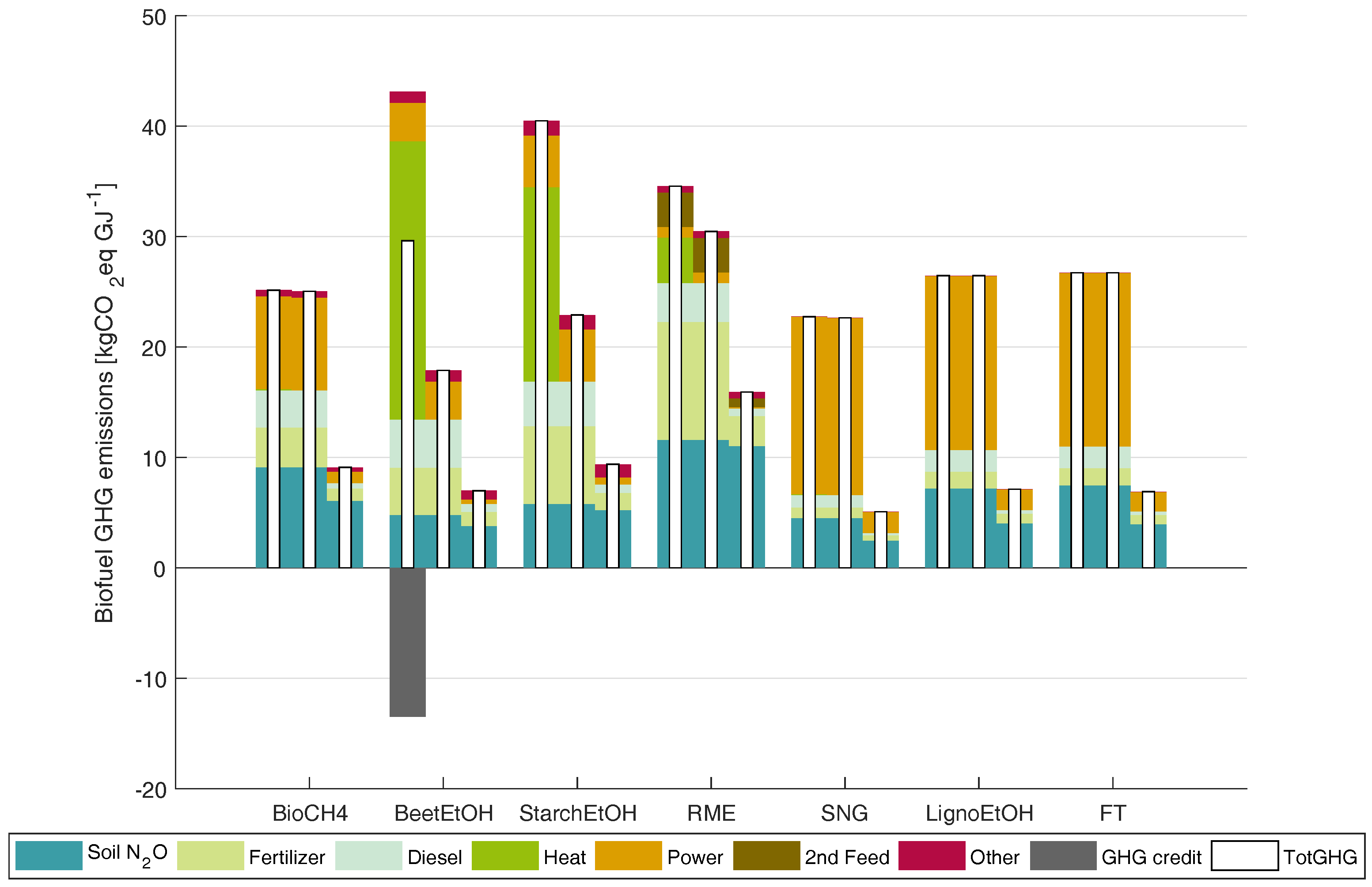
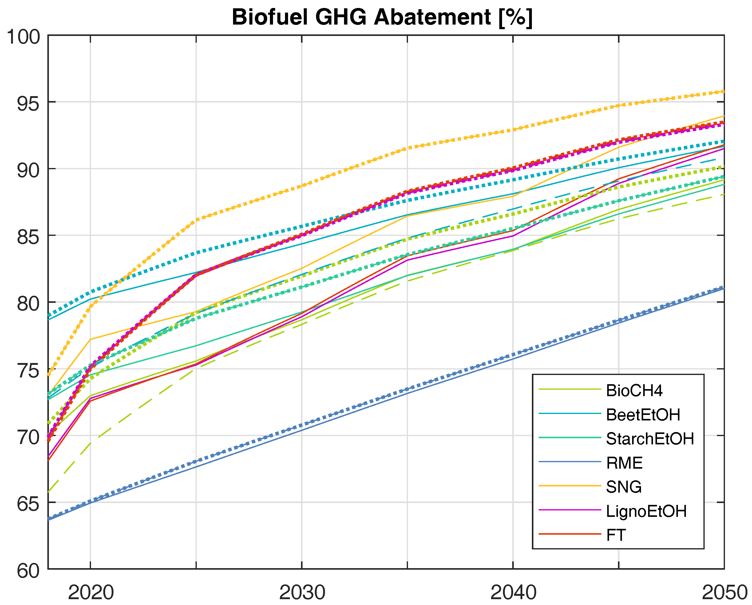
3.1. Biofuel GHG Emissions

The resulting GHG emissions are shown in Figure 2, showing that, in the beginning, BeetEtOH is the better performing option in terms of GHG abatement per energy unit, with SNG second and StarchEtOH third best. Currently dominant RME is in fact the worst option. Through the system improvements, the advanced options gradually improve and overtake BeetEtOH (Figure 2 and Figure 3). Assuming a fast power mix emission improvement through coal decommission as in Scenarios (b) and (c), SNG is fast the best option, whereas at moderate power mix developments, this takes considerably longer. Of the advanced options, SNG performs clearly better due to higher conversion efficiencies and lower power demand, whereas LignoEtOH and FT-diesel perform similarly to each other, due to similar conversion efficiencies and inputs. It should however be noted that the options, with the exception of RME, achieve between 67% and 79% GHG abatement in the beginning and, again excepting RME, between 88% and 96% GHG abatement in the end. Thus, the differences are relatively small, leaving ample room for cost developments to change the priority order when comparing relative GHG abatement costs.

It can be noted that the “other” factors are relatively marginal in comparison to the other sources (Figure 2). Thus, simplified calculations excluding the other inputs where data are not available (such as for the advanced options) provide a sufficient estimate for the total GHG emissions.

As a consequence of switching from natural gas to wood chips from dedicated crops for the heat input, the land required for the options increases corresponding to the heat requirement (Figure 4). For BeetEtOH, the land requirement increases by 49%, while at the same time increasing the GHG abatement by 22%; for StarchEtOH, the land required increases by 36% with a 41% GHG abatement increase; for BioCH₄, land use increases by 24% (the reference already assumed renewable heat). For RME, the land use increases by 9% through a renewable heat input, with an additional 3% through the methanol input, while increasing GHG abatement by 8%.

The GHG abatement per hectare is shown for the base case in Figure 5. RME and StarchEtOH can abate 2–3 tCO₂eq ha⁻¹, whereas BioCH₄ and BeetEtOH are the present day best, with 6–7 tCO₂eq ha⁻¹. With a clean power mix and renewable input fertilizer and fuel, in addition to yield and conversion efficiency improvements, BioCH₄ and SNG can potentially achieve over 12 tCO₂eq ha⁻¹. BeetEtOH can achieve a maximal 8 tCO₂eq ha⁻¹, somewhat more than the liquid advanced biofuel options.

Notably, the merit order of the fuels differs when compared on a hectare basis and an energetic basis, resulting from yield differences. Whereas BioCH₄ is the best both for the beginning of the simulation in the base scenario in terms of GHG abatement per hectare, as well as in the long run (Figure 5), it is only fourth best in terms of GHG abatement on an energetic basis for the beginning (Figure 3) (even after StarchEtOH), and it is only fifth best in the long run.

3.2. Biofuel Relative GHG Abatement Cost

From the competition modeling, relative GHG abatement cost developments emerge, which are highly different between scenarios. In Figure 6, the extreme span of possible outcomes in the scenarios is sketched between Scenarios (a) and (c), with a more progressive power mix development and lower sugar beet and silage maize yields in the latter case.

In Scenario (a), BeetEtOH is the least cost option until 2037, when it is overtaken by SNG due to the combined effects of input emission improvements, conversion efficiency and yield increases and technological learning. SNG remains the least-cost option, slowly diverging with, but never surpassed by BioCH₄. Due to the annual 4% reference feedstock price increase, the minimum selling prices of all options generally increase. The exception to this is all advanced fuels in the first few years, when mainly the power mix emission reductions lead to slight overall relative GHG abatement cost reductions.

The least cost option over time increases from ca. 370–620 € tCO₂eq⁻¹. The two liquid advanced biofuel options start from ca. 570 € and increase towards 900 €, while the currently dominant biofuels RME and StarchEtOH increase from around 550 and 580 € to over 1300 and 1200 € tCO₂eq⁻¹, respectively. The advanced liquid fuels remain at an around 50% higher cost than the least-cost fuel, whereas for RME and StarchEtOH, the difference increases substantially over time.

In Scenario (c), significant differences compared to (a) can be seen. Primarily, SNG starts off as the least cost option, or compared to medium sugar beet yields, quickly surpasses BeetEtOH. Due to a combination of more rapid input GHG emission decreases and technological learning, minimum selling prices remain around 400 € tCO₂eq⁻¹ until 2030, with a subsequent increase to 600 € tCO₂eq⁻¹ towards the end.

The two liquid advanced biofuel options increase towards 870 €, while RME and StarchEtOH develop similarly to in Scenario (a). The advanced liquid fuels also in this case remain at an around 50% higher cost than the least-cost fuel, while the difference increases over time for RME and StarchEtOH. For the advanced liquid fuels, it can be observed (Figure 6) that they remain at a higher cost than BeetEtOH even in Scenario (c).

Notably, between diesel fuels, FT-diesel is quickly competitive with RME in any case, and thus, the sub-quota for diesel and petrol would favor advanced options, albeit at a higher cost than without the sub-quota.

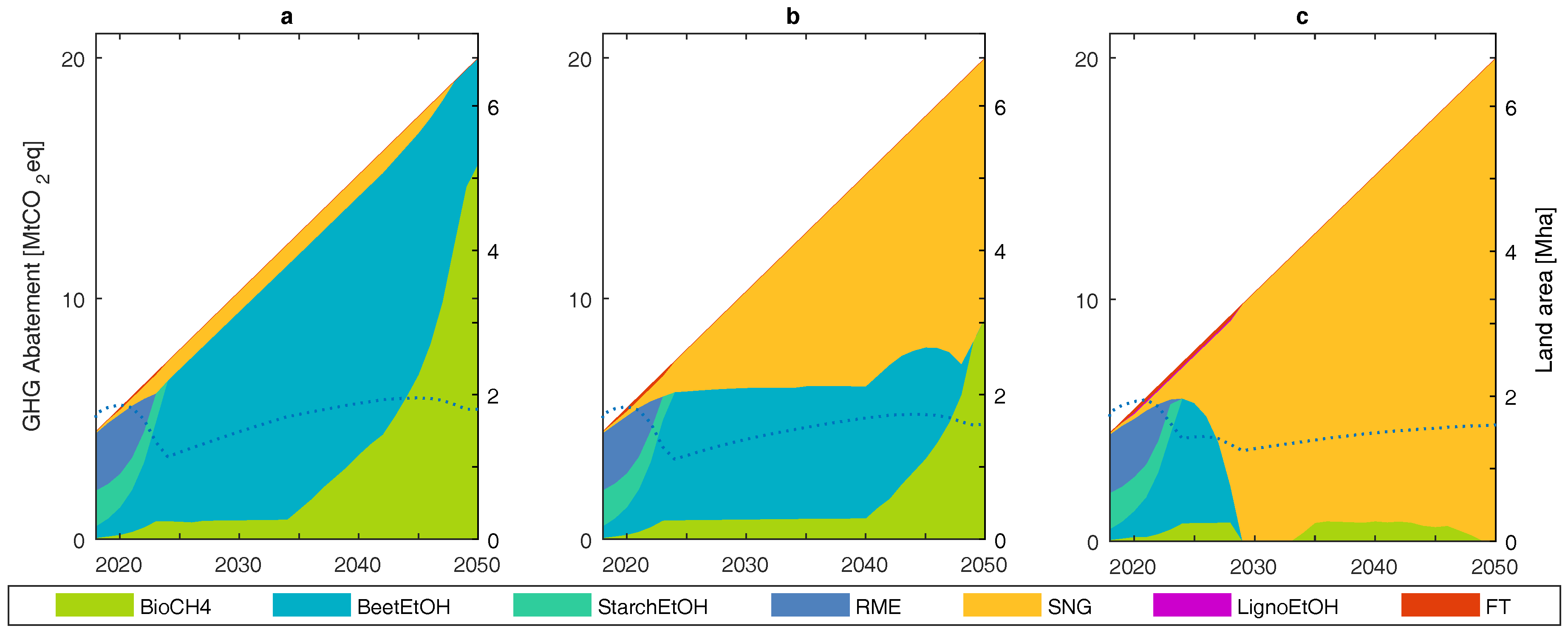
3.3. Scenario Modeling

From the GHG abatement cost competition, the resulting production developments can be seen in Figure 7. In all cases, both StarchEtOH and RME fall out of the market rather quickly. Instead, BeetEtOH, as well as in the scenarios where all fuels are included, SNG and BioCH₄, gain market shares in differing proportions between the scenarios. The advanced liquid options do not achieve significant market shares in any scenario.

In the base case (a), BeetEtOH dominates in the medium term, with SNG and BioCH₄ both gaining market shares, respectively, from ca. 2035 and 2040 onwards. For a more progressive power mix (b), SNG starts gaining market shares more rapidly, while BioCH₄ remains almost the same as in the base case. Gaseous fuels dominate fully towards the end. If additionally low yields for silage maize and sugar beet are assumed (c), SNG fully dominates the market within a decade.

The resulting required total arable land (including for heating purposes and secondary feedstocks) differs marginally between the scenarios, with an almost constant ca. 2 Mha used once RME and StarchEtOH are displaced (Figure 7). Thus, yield and conversion efficiency improvements compensate for the GHG abatement target increase.

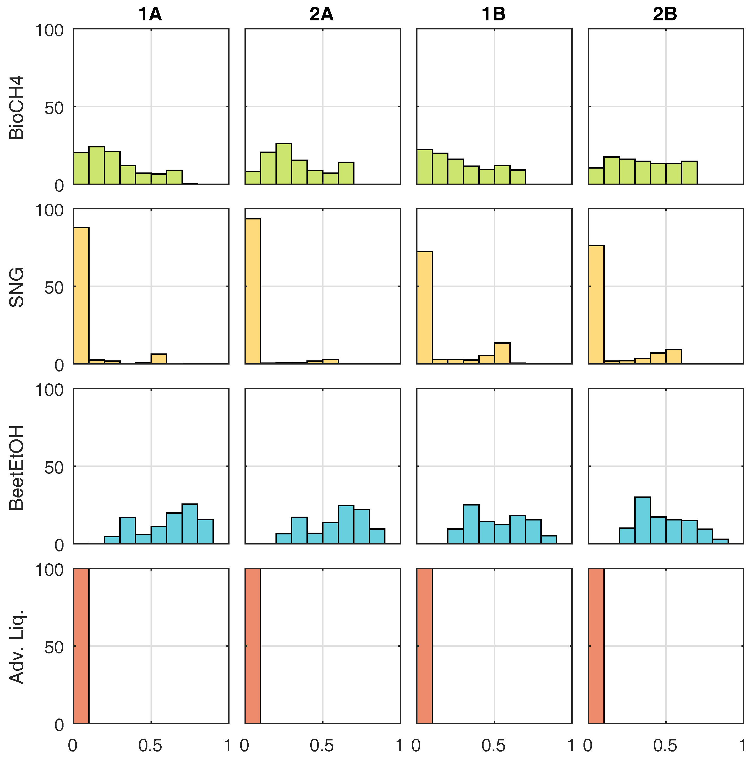
3.4. Sensitivity Analysis

From the sensitivity analysis, the resulting occurrences at different total market shares are shown for four cases (Figure 8), where the reference feedstock costs increase by 3% (“1”) and 4% (“2”) a⁻¹, while the power mix is either moderate (A) or progressive (B). For moderate power developments, BeetEtOH dominates, with BioCH₄ more often emerging at slightly higher cumulative market shares at higher feedstock cost increases. SNG remains at below 10% total market share in around 90% of the cases, with a slightly higher occurrence of market shares of over 10% at a lower feedstock cost increase. For SNG, there is a jump in the amount of occurrences at over 50% cumulative market shares, indicating that under favorable conditions, a threshold is surpassed early, leading to learning effects and increasing returns.

At more progressive power mix developments, BeetEtOH still dominates in most cases, but the occurrences at the higher market shares are fewer. BioCH₄ occurs at higher shares more often compared to a moderate power mix development, especially at a higher feedstock cost increase. The effect on the competitiveness of SNG is substantial, with substantially more occurrences between 10% and 60% cumulative market shares, especially at a lower feedstock cost increase.

In very few of the cases do the gaseous fuels arrive at cumulative market shares of above 60%, and BeetEtOH achieves cumulative market shares of above 30% in almost all cases.

For the advanced liquid biofuels, the share remains at below 5% in all of the observed cases, despite the fact that only liquid fuels were included.

The biofuel cost sensitivity is shown in Figure 9. In contrast to an energetic basis [3], the sensitivity of the relative GHG abatement cost of RME is high, due mainly to the uncertain soil emissions, which contribute more to RME due to low yields. The relative GHG abatement costs of the advanced liquid biofuels are also highly uncertain, with more than a factor of three difference for the low and high end even at the beginning. In contrast, SNG shows clearly less uncertainty, despite stemming from the same feedstock. BeetEtOH, followed by BioCH₄, shows the lowest span, across time-points.

4. Discussion

In this paper, feedstock cost developments of biofuels have been combined with GHG abatement developments in order to estimate future spans of relative GHG abatement costs for the different options and their competitiveness. From the point of view of a cost-optimal GHG abatement through the deployment of biofuels, the current practice emerged as increasingly divergent from the best options.

Whereas advanced biofuels were found to be competitive only at low feedstock price increases when comparing the fuels on an energetic basis [3], especially SNG was found to be competitive even at higher feedstock price increases on a GHG abatement basis. Furthermore, the power mix development is in fact more important for the competitiveness of advanced biofuels than are feedstock cost increase differences. This is due to the fact that the power mix emissions have a substantially different impact on the various biofuel options, as the power input requirements differ. Differing soil emissions result in additionally divergent GHG abatement and especially GHG abatement and thus relative GHG abatement cost uncertainty.

Liquid advanced biofuels were competitive only when gaseous fuels were not included and, even then, only at very favorable conditions. In the sensitivity analysis, all relevant factors except lower sugar beet yields were varied, resulting in an almost complete absence of advanced liquid biofuels. Thus, the competitiveness of advanced liquid biofuels requires low sugar beet yields to be enforced, in addition to low feedstock cost increases and a progressive power mix development, as well as gaseous fuels being excluded. Potentially, process internal power generation through the use of byproducts could improve the GHG balance; however, in such a case, the economic benefit from byproduct sales would be removed, and thus, a trade-off presents itself for the GHG abatement cost, possibly with a zero sum total result. A diversion to producing more power and thus less fuels results in a similar trade-off.

The biofuel amounts required towards the end of the time span correspond to about 13% of current fuel demand (or in the case of large expansion of, e.g., electric vehicles, a correspondingly higher market share). A continuation of the present quota would require marginally more, due to the slightly lower GHG abatement of advanced FT-diesel, but at an at least 50% higher cost compared to without the sub-quota for diesel and gasoline fuels. The resulting least-cost practices would imply mixing BeetEtOH into petrol at higher shares than today, requiring a larger share of flex-fuel vehicles in the fleet ([47], p. 21), which are however readily available and at similar sales prices [48]. For gaseous fuels, the current demand needs to increase manifold in order to accommodate the least-cost developments. Methane-driven vehicles are available in differing shares across different countries ([49], p. 44ff), with as little as 400 € (ca. 2%) higher prices compared to their conventional counterparts [50], thus not substantially affecting the competitiveness results in this paper (especially when considering potential cost-reductions through production up-scaling). If a large increase of gas fuel use is proven not to be possible, BeetEtOH is a possible long-term second-best option, albeit with significantly lower GHG abatement potential per unit of arable land compared to the gaseous options.

A slight trade-off was found between optimizing the GHG emissions from the input heat and the resulting additional land required for the lignocellulosic crops used for this purpose, which in the case of BeetEtOH amounted to 49%, while increasing the GHG abatement by 22%. Thus, this additional land is motivated, but the benefits may be somewhat reduced through emissions related to land use.

Indirect land use change (iLUC) emissions have been highlighted as a problem with crop cultivation. If applied for the attribution to the GHG abatement of the biofuel options, these emissions are a function of yield, as well as are to some extent direct soil emissions (the latter is also related to agricultural practices, which can be substantially improved [51], as well as to, e.g., regional soil and climate differences [52]). Thus, both are arguments for increasing the hectare GHG abatement of biofuels, through swapping from the presently used low-yielding crops to higher yielding options. The highest yielding options included here are BioCH₄ and SNG, both gaseous fuels. The former is based on silage maize, which (similarly to sugar beet) consumes soil humus ([35], p. 272ff) and in the worst case has relatively high soil N₂O emissions. Soil erosion and N₂O emission need to be monitored and curbed in order to ensure sustainable biofuel practices. A more holistic approach including all relevant environmental factors is necessary in order to avoid sub-optimal practices, and the risk of high soil emissions needs to be taken into account and assessed.

GHG abatement cost in terms of € tCO₂eq⁻¹ does not give the full picture, as the GHG abatement in energetic terms deviates from that in terms of required arable land, which sets a hard limit for biofuels from dedicated crops. For BioCH₄, the difference between the GHG abatement on an energetic basis compared to on a land use basis is particularly large (cf. Figure 3 and Figure 5). The GHG abatement cost difference between BioCH₄ and BeetEtOH, as well as SNG was also found to be large (Figure 6) compared to the GHG abatement per land used.

The total possible GHG abatement is limited by available arable land and residual biomass, and thus, for an overall optimal GHG abatement, total yields need to be taken into account. A GHG abatement cost also ignores other relevant environmental metrics (see, e.g., [53]), such as biodiversity, soil erosion, pesticide use, freshwater use and land use change. In such a comparison, it would be beneficial to compare biofuel options according to land area, as some biofuels may perform worse in some metrics, but through higher yields would free land, which can be for instance conserved (cf., [54]), thus potentially rendering the overall impact better.

Thus, in terms of several both direct and indirect environmental aspects, as well as in terms of economic [3] and social aspects (e.g., food competition), a switch to higher yielding fuels would be beneficial, especially if at the same time other relevant environmental effects are monitored and curbed. In order to achieve such a shift, presently used biofuels need to be exchanged with either bioethanol or gaseous fuels if the least-cost target and highest GHG abatement are to be achieved, or if this is proven to be infeasible, replacing RME with FT-diesel would be necessary in terms of both GHG abatement cost, as well as absolute GHG abatement. For the advanced options, especially liquid ones, both unpredictable feedstock costs and highly uncertain investment costs may inhibit such a development [3]. However, in terms of GHG abatement, the benefits are more clear than in energetic terms.

As noted in Millinger and Thrän [3], perennials currently have a higher market price than those resulting with the method used, which can be at least partly explained by small markets, as well as farmer risk considerations. Until the market demand for perennial lignocellulosic biomass is stable enough for the investment risk to be reduced, higher prices should be expected, thus potentially postponing the deployment of biofuels based on such crops.

The use of so-called degraded or marginal lands has been suggested in order to avoid land use change emissions and food competition [55]. Although yields would be strongly affected compared to currently used arable land [56], the competitiveness compared to non-perennials is obvious, as the latter would likely not be cultivated on such lands.

5. Conclusions

In this paper, a thorough assessment of long-term relative GHG abatement cost developments of biofuel options in Germany has been carried out. The better performing of the included biofuel options in terms of GHG abatement cost was sugar beet-based ethanol for the short to medium term, and silage maize-based BioCH₄ and/or woody feedstock-based SNG for the medium to long term. BioCH₄ was found to be especially competitive at higher feedstock price increases and progressive power mix developments, while lower feedstock price increases were favorable for SNG. BeetEtOH was especially competitive at less progressive power mix developments.

The currently most common biofuels were found to have over 40% higher relative GHG abatement costs than the least cost option (BeetEtOH) for the beginning, and increasing substantially over time, due to higher relative feedstock cost increases.

Liquid advanced biofuel options were only found to be competitive at a combination of favorable circumstances, and were in normal circumstances about 50% more expensive than the least-cost option (depending on time-point and scenario, either BeetEtOH, SNG or BioCH₄) throughout the whole time span. Only if low sugar beet yields were enforced, in addition to low feedstock cost increases and a progressive power mix development, as well as gaseous fuels being excluded, were advanced liquid fuels found to become competitive.

The competitiveness of advanced biofuels was found to be more sensitive to the emissions development of the power mix than on feedstock costs, as this factor is more differentiated between the high-performing fuels.

Through switching from the currently most common biofuels RME and StarchEtOH to BioCH₄ and SNG, the GHG abatement per land area can potentially be increased by a factor of five. For the present day, a switch to BioCH₄ and BeetEtOH with renewable heat sources trebles the spatial GHG abatement, despite the fact that the heat source requires substantial amounts of land.

A discrepancy between GHG abatement in relation to energetic output compared to land output was found, having important consequences especially for the competitiveness of BioCH₄. BioCH₄ was mostly not GHG abatement cost competitive and did not achieve high market shares in any scenario, while on a land use basis, it was the best already in the beginning, as well as in the long term. Although the land use was reflected to some extent in the cost competitiveness, larger differences and a substantially switched merit order resulted when comparing them on an area basis.

Due to the large spread of possible pathway emissions, as well as cost developments, measures to quantify and curb emissions in each section of the pathway are called for in order to reduce uncertainties, starting from the specific field used, through the conversion, as well as in the end use.

Finally, there are strong arguments, both social, economic and environmental, for including the required arable land for biofuels into policy and functional units, instead of merely energy or GHG abatement (cf., [9]). Such a differentiation between crop-based biofuels can potentially lead to a substantially higher GHG abatement from the same arable land area, through incentives to switch to higher yielding gaseous options.

References

1. European Environment Agency (EEA). European Environment Agency Greenhouse Gas Data Viewer; European Environment Agency: Copenhagen, Denmark, 2017; Available online: www.eea.europa.eu/data-and-maps/data/data-viewers/greenhouse-gases-viewer (accessed on 10 November 2017).
2. Bundesanstalt für Landwirtschaft und Ernährung (BLE). Hintergrunddaten zum Evaluations-und Erfahrungsbericht 2016; Bundesanstalt für Landwirtschaft und Ernährung: Bonn, Germany, 2017. [Google Scholar]
3. Millinger, M.; Thrän, D. Biomass price developments inhibit biofuel investments and research in Germany: The crucial future role of high yields. J. Clean. Prod. 2018, 172, 1654–1663. [Google Scholar] [CrossRef]
4. Bundesministerium für Verkehr, Bau und Stadtentwicklung (BMVBS). Die Mobilitäts-und Kraftstoffstrategie der Bundesregierung (MKS): Energie auf Neuen Wegen; Bundesministerium für Verkehr, Bau und Stadtentwicklung: Berlin, Germany, 2013. [Google Scholar]
5. Millinger, M.; Ponitka, J.; Arendt, O.; Thrän, D. Competitiveness of advanced and conventional biofuels: Results from least-cost modeling of biofuel competition in Germany. Energy Policy 2017, 107, 394–402. [Google Scholar] [CrossRef]
6. Menten, F.; Chèze, B.; Patouillard, L.; Bouvart, F. A review of LCA greenhouse gas emissions results for advanced biofuels: The use of meta-regression analysis. Renew. Sustain. Energy Rev. 2013, 26, 108–134. [Google Scholar] [CrossRef]
7. Cherubini, F.; Strømman, A.H. Life cycle assessment of bioenergy systems: State of the art and future challenges. Bioresour. Technol. 2011, 102, 437–451. [Google Scholar] [CrossRef] [PubMed]
8. Crutzen, P.J.; Mosier, A.R.; Smith, K.A.; Winiwarter, W. N2O release from agro-biofuel production negates global warming reduction by replacing fossil fuels. Atmos. Chem. Phys. 2008, 8, 389–395. [Google Scholar] [CrossRef]
9. BImSchV. Achtunddreißigste Verordnung zur Durchführung des Bundes-Immissionsschutzgesetzes (Verordnung zur Festlegung weiterer Bestimmungen zur Treibhausgasminderung bei Kraftstoffen): 38. BImSchV. Bundesgesetzblatt 2017, 1, 3892. [Google Scholar]
10. Yan, X.; Inderwildi, O.R.; King, D.A. Biofuels and synthetic fuels in the US and China: A review of Well-to-Wheel energy use and greenhouse gas emissions with the impact of land-use change. Energy Environ. Sci. 2010, 3, 190–197. [Google Scholar]
11. Malça, J.; Freire, F. Life-cycle studies of biodiesel in Europe: A review addressing the variability of results and modeling issues. Renew. Sustain. Energy Rev. 2011, 15, 338–351. [Google Scholar] [CrossRef]
12. Haarlemmer, G.; Boissonnet, G.; Imbach, J.; Setier, P.A.; Peduzzi, E. Second generation BtL type biofuels—A production cost analysis. Energy Environ. Sci. 2012, 5, 8445–8456. [Google Scholar] [CrossRef]
13. Haarlemmer, G.; Boissonnet, G.; Peduzzi, E.; Setier, P.A. Investment and production costs of synthetic fuels—A literature survey. Energy 2014, 66, 667–676. [Google Scholar] [CrossRef]
14. Festel, G.; Würmseher, M.; Rammer, C.; Boles, E.; Bellof, M. Modeling production cost scenarios for biofuels and fossil fuels in Europe. J. Clean. Prod. 2014, 66, 242–253. [Google Scholar] [CrossRef]
15. Browne, J.; Nizami, A.S.; Thamsiriroj, T.; Murphy, J.D. Assessing the cost of biofuel production with increasing penetration of the transport fuel market: A case study of gaseous biomethane in Ireland. Renew. Sustain. Energy Rev. 2011, 15, 4537–4547. [Google Scholar] [CrossRef]
16. Dwivedi, P.; Khanna, M. Abatement cost of GHG emissions for wood-based electricity and ethanol at production and consumption levels. PLoS ONE 2014, 9, e100030. [Google Scholar] [CrossRef] [PubMed]
17. Dwivedi, P.; Wang, W.; Hudiburg, T.; Jaiswal, D.; Parton, W.; Long, S.; DeLucia, E.; Khanna, M. Cost of abating greenhouse gas emissions with cellulosic ethanol. Environ. Sci. Technol. 2015, 49, 2512–2522. [Google Scholar] [CrossRef] [PubMed]
18. Rehl, T.; Müller, J. CO2 abatement costs of greenhouse gas (GHG) mitigation by different biogas conversion pathways. J. Environ. Manag. 2013, 114, 13–25. [Google Scholar] [CrossRef] [PubMed]
19. Tomaschek, J.; Özdemir, E.D.; Fahl, U.; Eltrop, L. Greenhouse gas emissions and abatement costs of biofuel production in South Africa. GCB Bioenergy 2012, 4, 799–810. [Google Scholar] [CrossRef]
20. Schmidt, J.; Leduc, S.; Dotzauer, E.; Kindermann, G.; Schmid, E. Cost-effective CO2 emission reduction through heat, power and biofuel production from woody biomass: A spatially explicit comparison of conversion technologies. Appl. Energy 2010, 87, 2128–2141. [Google Scholar] [CrossRef]
21. Martinez-Hernandez, E.; Campbell, G.M.; Sadhukhan, J. Economic value and environmental impact (EVEI) analysis of biorefinery systems. Chem. Eng. Res. Des. 2013, 91, 1418–1426. [Google Scholar] [CrossRef]
22. Martinez-Hernandez, E.; Campbell, G.M.; Sadhukhan, J. Economic and environmental impact marginal analysis of biorefinery products for policy targets. J. Clean. Prod. 2014, 74, 74–85. [Google Scholar] [CrossRef] [Green Version]
23. Budzinski, M.; Nitzsche, R. Comparative economic and environmental assessment of four beech wood based biorefinery concepts. Bioresour. Technol. 2016, 216, 613–621. [Google Scholar] [CrossRef] [PubMed]
24. Zech, K.; Meisel, K.; Brosowski, A.; Villadsgaard Toft, L.; Müller-Langer, F. Environmental and economic assessment of the Inbicon lignocellulosic ethanol technology. Appl. Energy 2016, 171, 347–356. [Google Scholar] [CrossRef]
25. McKinsey & Company. Costs and Potentials of Greenhouse Gas Abatement in Germany: A Report by McKinsey & Company, Inc., on Behalf of “BDI Initiativ—Business for Climate”; McKinsey & Company, Inc.: New York, NY, USA, 2007; Available online: www.mckinsey.com (accessed on 21 February 2018).
26. McKinsey & Company. Pathways to a Low-Carbon Economy: Version 2 of the Global Greenhouse Gas Abatement Cost Curve; McKinsey & Company, Inc.: New York, NY, USA, 2009; Available online: www.mckinsey.com (accessed on 23 March 2017).
27. Thrän, D.; Schaldach, R.; Millinger, M.; Wolf, V.; Arendt, O.; Ponitka, J.; Gärtner, S.; Rettenmaier, N.; Hennenberg, K.; Schüngel, J. The MILESTONES modeling framework: An integrated analysis of national bioenergy strategies and their global environmental impacts. Environ. Model. Softw. 2016, 86, 14–29. [Google Scholar] [CrossRef]
28. Thrän, D.; Arendt, O.; Banse, M.; Braun, J.; Fritsche, U.; Gärtner, S.; Hennenberg, K.J.; Hünneke, K.; Millinger, M.; Ponitka, J.; et al. Strategy Elements for a Sustainable Bioenergy Policy Based on Scenarios and Systems Modeling: Germany as Example. Chem. Eng. Technol. 2017, 40, 211–226. [Google Scholar] [CrossRef]
29. DIN’s Standards Committee Principles of Environmental Protection (NAGUS). DIN EN 16214-4. In Sustainability Criteria for the Production of Biofuels and Bioliquids for Energy Applications—Principles, Criteria, Indicators and Verifiers—Part 4: Calculation Methods of the Greenhouse Gas Emission Balance Using a Life Cycle Analysis Approach; German Version EN 16214-4:2013; NAGUS: Berlin, Germany, 2013. [Google Scholar]
30. Ponitka, J.; Arendt, O.; Lenz, V.; Daniel-Gromke, J.; Stinner, W.; Ortwein, A.; Zeymer, M.; Gröngröft, A.; Müller-Langer, F.; Klemm, M.; et al. Focus on: Bioenergy-Technologies: Conversion Pathways—Towards Biomass Energy Use in the 21st Century, 2nd ed.; DBFZ: Leipzig, Germany, 2016. [Google Scholar]
31. International Council on Clean Transportation Europe (ICCT). European Vehicle Market Statistics: Pocketbook 2016/2017; International Council on Clean Transportation Europe: Berlin, Germany, 2016. [Google Scholar]
32. Majer, S.; Gröngröft, A.; Drache, C.; Braune, M.; Meisel, K.; Müller-Langer, F.; Naumann, K.; Oehmichen, K. Technical Principles and Methodology for Calculating GHG Balances of Biodiesel: Guidance Document: Version 1.0; DBFZ: Leipzig, Germany, 2016. [Google Scholar]
33. Meisel, K.; Braune, M.; Gröngröft, A.; Majer, S.; Müller-Langer, F.; Naumann, K.; Oehmichen, K. Technical Principles and Methodology for Calculating GHG Balances of Bioethanol: Guidance Document: Version 1.0; DBFZ: Leipzig, Germany, 2016. [Google Scholar]
34. Oehmichen, K.; Naumann, K.; Postel, J.; Drache, C.; Braune, M.; Gröngröft, A.; Majer, S.; Meisel, K.; Müller-Langer, F. Technical Principles and Methodology for Calculating GHG Balances of Biomethane: Guidance Document: Version 1.0; DBFZ: Leipzig, Germany, 2016. [Google Scholar]
35. Kuratorium für Technik u. Bauwesen i. d. Landwirtschaft e.V. (KTBL). Energiepflanzen: Daten für die Planung des Energiepflanzenanbaus: KTBL Datensammlung, 2nd ed.; KTBL: Darmstadt, Germany, 2012. [Google Scholar]
36. Neeft, J.; Ludwiczek, N. BioGrace II—Harmonized Greenhouse Gas Calculations for Electricity, Heating and Cooling from Biomass; European Union: Brussels, Belgium, 2015; Available online: www.biograce.net (accessed on 13 December 2017).
37. Parsons Brinckerhoff. Accelerating the Uptake of CCS: Industrial Use of Captured Carbon Dioxide; Global CCS Institute: Docklands, Australia, 2011. [Google Scholar]
38. Brosowski, A.; Thrän, D.; Mantau, U.; Mahro, B.; Erdmann, G.; Adler, P.; Stinner, W.; Reinhold, G.; Hering, T.; Blanke, C. A review of biomass potential and current utilisation—Status quo for 93 biogenic wastes and residues in Germany. Biomass Bioenergy 2016, 95, 257–272. [Google Scholar] [CrossRef]
39. Bundesministerium für Wirtschaft und Energie (BMWi). Energiedaten: Gesamtausgabe: Stand: Oktober 2017; Bundesministerium für Wirtschaft und Energie: Berlin, Germany, 2017. [Google Scholar]
40. Majer, S.; Gröngröft, A. Ökologische und ökonomische Bewertung der Produktion von Biomethanol für die Biodieselherstellung; Deutsches Biomasseforschungszentrum (DBFZ): Leipzig, Germany, 2010. [Google Scholar]
41. Cherkasov, N.; Ibhadon, A.O.; Fitzpatrick, P. A review of the existing and alternative methods for greener nitrogen fixation. Chem. Eng. Process. Process Intensif. 2015, 90, 24–33. [Google Scholar] [CrossRef]
42. Dulles, V.A. Sustainable Ammonia Synthesis: Exploring the Scientific Challenges Associated with Discovering Alternative, Sustainable Processes for Ammonia Production: DOE Roundtable Report; United States Department of Energy: Washington, DC, USA, 2016.
43. World Wildlife Foundation (WWF). Zukunft Stromsystem: Kohleausstieg 2035—Vom Ziel her Denken; World Wildlife Foundation: Berlin, Germany, 2017. [Google Scholar]
44. Neeft, J.; te Buch, S.; Gerlagh, T.; Gagnepain, B.; Bacovsky, D.; Ludwiczek, N.; Lavelle, P.; Thonier, G.; Lechon, Y.; Lago, C.; et al. BioGrace—Harmonized Calculations of Biofuel Greenhouse Gas Abatement: Publishable Final Report for Grant Agreement IEE/09/736; European Union: Brussels, Belgium, 2012; Available online: www.biograce.net (accessed on 13 December 2017).
45. European Union (EU). Directive 2009/28/EC of the European Parliament and of the Council of 23 April 2009 on the Promotion of the Use of Energy from Renewable Sources and Amending and Subsequently Repealing Directives 2001/77/EC and 2003/30/EC; European Union: Brussels, Belgium, 2009. [Google Scholar]
46. Bundesministerium für Umwelt, Naturschutz, Bau und Reaktorsicherheit (BMUB). Klimaschutzplan 2050—Klimaschutzpolitische Grundsätze und Ziele der Bundesregierung; BMUB: Rostock, Germany, 2016; Available online: www.bmub.bund.de (accessed on 4 September 2017).
47. Intergovernmental Panel on Climate Change (IPCC). Climate Change 2014: Mitigation of Climate Change: Chapter 8—Transport. In Climate Change 2014: Mitigation of Climate Change; IPCC, Ed.; IPCC: Geneva, Switzerland; Cambridge University Press: Cambridge, UK; New York, NY, USA, 2014. [Google Scholar]
48. U.S. DOE. Fuel Economy of New Flex-Fuel Vehicles; U.S. Department of Energy: Washington, DC, USA, 2018. Available online: www.fueleconomy.gov (accessed on 23 February 2018).
49. International Council on Clean Transportation Europe (ICCT). European Vehicle Market Statistics: Pocketbook 2017/2018; International Council on Clean Transportation Europe: Berlin, Germany, 2017. [Google Scholar]
50. Allgemeiner Deutscher Automobil-Club e.V. (ADAC). ADAC Kostenvergleich: Erd-und Autogas Gegen Benziner und Diesel; Allgemeiner Deutscher Automobil-Club e.V.: Munich, Germany, 2018; Available online: www.adac.de (accessed on 23 February 2018).
51. Skenhall, S.A.; Berndes, G.; Woods, J. Integration of bioenergy systems into UK agriculture—New options for management of nitrogen flows. Biomass Bioenergy 2013, 54, 219–226. [Google Scholar] [CrossRef]
52. O’Keeffe, S.; Majer, S.; Drache, C.; Franko, U.; Thrän, D. Modeling biodiesel production within a regional context—A comparison with RED Benchmark. Renew. Energy 2017, 108, 355–370. [Google Scholar] [CrossRef]
53. Rockstrom, J.; Steffen, W.; Noone, K.; Persson, A.; Chapin, F.S.; Lambin, E.F.; Lenton, T.M.; Scheffer, M.; Folke, C.; Schellnhuber, H.J.; et al. A safe operating space for humanity. Nature 2009, 461, 472–475. [Google Scholar] [CrossRef] [PubMed]
54. Vadenbo, C.; Tonini, D.; Astrup, T.F. Environmental Multiobjective Optimization of the Use of Biomass Resources for Energy. Environ. Sci. Technol. 2017, 51, 3575–3583. [Google Scholar] [CrossRef] [PubMed]
55. Tilman, D.; Hill, J.; Lehman, C. Carbon-Negative Biofuels from Low-Input High-Diversity Grassland Biomass. Science 2006, 314, 1598–1600. [Google Scholar] [CrossRef] [PubMed]
56. Searle, S.Y.; Malins, C.J. Will energy crop yields meet expectations? Biomass Bioenergy 2014, 65, 3–12. [Google Scholar] [CrossRef]
57. Grubler, A. Technology and Global Change; Cambridge University Press: Cambridge, UK, 1998. [Google Scholar]
58. International Energy Agency (IEA). Experience Curves for Energy Technology Policy; IEA Publications: Paris, France, 2000. [Google Scholar]
59. Hamelinck, C.N.; van Hooijdonk, G.; Faaij, A.P.C. Ethanol from lignocellulosic biomass: Techno-economic performance in short-, middle- and long-term. Biomass Bioenergy 2005, 28, 384–410. [Google Scholar] [CrossRef]
60. Lange, J.P. Fuels and Chemicals Manufacturing: Guidelines for Understanding and Minimizing the Production Costs. CatTech 2001, 5, 82–95. [Google Scholar] [CrossRef]
61. Bridgwater, A. Technical and Economic Assessment of Thermal Processes for Biofuels: NNFCC Project 08/018; Consultants on Process Engineering Ltd.: Calgary, AB, Canada, 2009; Available online: http://www.globalbioenergy.org (accessed on 10 September 2015).
62. Witzel, C.P.; Finger, R. Economic evaluation of Miscanthus production—A review. Renew. Sustain. Energy Rev. 2016, 53, 681–696. [Google Scholar] [CrossRef]
63. Ericsson, K.; Rosenqvist, H.; Nilsson, L.J. Energy crop production costs in the EU. Biomass Bioenergy 2009, 33, 1577–1586. [Google Scholar] [CrossRef]
64. Krasuska, E.; Rosenqvist, H. Economics of energy crops in Poland today and in the future. Biomass Bioenergy 2012, 38, 23–33. [Google Scholar] [CrossRef]
65. Faasch, R.J.; Patenaude, G. The economics of short rotation coppice in Germany. Biomass Bioenergy 2012, 45, 27–40. [Google Scholar] [CrossRef]
66. James, L.K.; Swinton, S.M.; Thelen, K.D. Profitability Analysis of Cellulosic Energy Crops Compared with Corn. Agron. J. 2010, 102, 675–687. [Google Scholar] [CrossRef]
67. Khanna, M.; Dhungana, B.; Clifton-Brown, J. Costs of producing miscanthus and switchgrass for bioenergy in Illinois. Biomass Bioenergy 2008, 32, 482–493. [Google Scholar] [CrossRef]
68. Destatis. Statistisches Jahrbuch 2017: Deutschland und Internationales, 1st ed.; Statistisches Bundesamt: Wiesbaden, Germany, 2017.
Figure 1. System boundaries of the well-to-tank (WTT) assessment from feedstock cultivation to the tank for each pathway, shown by the dashed line S. The resulting abatement is compared on the basis of different functional units, such as GHG abatement per energy unit, cost per GHG abatement and GHG abatement per land area used. F = feedstock cultivation; T = transport; P1 = Process 1; P2 = Process 2; E = end use; m ˙ k = process inputs; m ˙ b y = process byproducts; α = allocation factor. The end use, as well as potential indirect land use effects are not included. The biofuel combustion is assumed to be carbon neutral, as the carbon absorbed during plant growth is emitted, thus closing the cycle.
Energies 11 00615 g001
Figure 2. GHG emissions for the biofuel options, broken down to their sources (kgCO2eq GJ−1). The leftmost bar for each option is the reference literature case; the middle bar shows the results for the start year of the base case, with renewable heat input; the rightmost bar shows the results for the last year of the base case, where the power mix is cleaner, yields and conversions efficiencies improved and renewable fuel and fertilizer inputs assumed.
Energies 11 00615 g002
Figure 3. Biofuel GHG abatement development, compared on an energetic basis with the fossil reference. The solid lines show the development in Scenario (a), at a moderate power mix development; the dotted lines show the development in Scenario (b), at a more progressive power mix development; the dashed lines show the development in Scenario (c), with additionally lower sugar beet and silage maize yields. The non-smooth developments of some of the curves (of the options with a large power input) are due to interpolation of power mix values, which are given for every five years.
Energies 11 00615 g003
Figure 4. Biofuel land requirement by source in the first year of the base case.
Energies 11 00615 g004
Figure 5. Biofuel GHG abatement per hectare in the base case with medium yields for all crops. The bar shows the initial GHG abatement, whereas the whisker extends to the GHG abatement in the last year.
Energies 11 00615 g005
Figure 6. Biofuel relative GHG abatement cost developments (€ tCO2eq−1) in scenarios (a, solid lines) and (c, dotted lines). Some developments are outside of the plot: the cost of RME increases to ca. 1300 € tCO2eq−1, and the cost of StarchEtOH increases to ca. 1230 € tCO2eq−1 in both cases.
Energies 11 00615 g006
Figure 7. Biofuel competitiveness based on relative GHG abatement cost in the scenarios. The areas show the total performed GHG abatement through each option (left axis), whereas the dotted line shows the total arable land required (right axis). The base scenario (a) assumes a moderate power mix development according to ([43], p. 123), a wheat price increase of 4% a−1, GHG optimized process heat and medium yields for all crops. In Scenario (b), the power mix is more progressive, and in Scenario (c), additionally, the sugar beet and silage maize yields are assumed within the low range in Table 1.
Energies 11 00615 g007
Figure 8. Sensitivity of biofuel production shares, at annual 3% (1) and 4% (2) wheat price increases, with moderate (A) and more progressive (B) power mix developments. 2A and 2B correspond to the sensitivities within Scenarios (a) and (b). The share (%) of the occurrences among the 1000 runs at total cumulative biofuel shares (on an energetic basis) of between 0% and 10%, 10% and 20% etc., are shown in the histogram. The shares are of the total cumulative biofuel deployment over the whole time span. For the upper three, all fuels were included, whereas for advanced liquid fuels, only liquid biofuels were included.
Energies 11 00615 g008
Figure 9. Sensitivity of total cost of the GHG abatement of biofuels in 2018, 2030 and 2050 in Sensitivity Case 1B (corresponding to the base scenario (a)), at a constant annual 4% wheat price increase and the other variables randomly varied according to Section 2.4. The red lines show the median; the bottom and top edges of the blue box show the 25th and 75th percentiles, respectively; the whiskers extend to a maximum of 1.5-times the length of the box; and outside of this interval, outliers are plotted with a red cross.
Energies 11 00615 g009